Extreme quantum nonequilibrium, nodes, vorticity, drift, and relaxation retarding states
Abstract
Consideration is given to the behaviour of de Broglie trajectories that are separated from the bulk of the Born distribution with a view to describing the quantum relaxation properties of more ‘extreme’ forms of quantum nonequilibrium. For the 2-dimensional isotropic harmonic oscillator, through the construction of what is termed the ‘drift field’, a description is given of a general mechanism that causes the relaxation of ‘extreme’ quantum nonequilibrium. Quantum states are found which do not feature this mechanism, so that relaxation may be severely delayed or possibly may not take place at all. A method by which these states may be identified, classified and calculated is given in terms of the properties of the nodes of the state. Properties of the nodes that enable this classification are described for the first time.
1 Introduction
De Broglie-Bohm theory [1, 2, 3, 4] is the archetypal member of a class [5, 6, 7, 8] of interpretations of quantum mechanics that feature a mechanism by which quantum probabilities arise dynamically [5, 9, 10, 11, 12, 13, 14] from standard ignorance-type probabilities. This mechanism, called ‘quantum relaxation’, occurs spontaneously through a process that is directly analogous to the classical relaxation (from statistical nonequilibrium to statistical equilibrium) of a simple isolated mechanical system as described by the second thermodynamical law. Demonstration of the validity of quantum relaxation [11, 15, 5, 14, 12, 13] has meant that the need to postulate agreement with quantum probabilities outright may be dispensed with. It has also prompted the consideration of ‘quantum nonequilibrium’--that is, violations of standard quantum probabilities, which in principle could be observed experimentally11 1 This conclusion is not entirely without its critics. For an alternative viewpoint see references [16, 17]. For counterarguments to this viewpoint see references [18, 19].. In other words, these theories allow for arbitrary nonequilibrium probabilities, only reproducing the predictions of standard quantum theory in their state of maximum entropy. It has been conjectured that the universe could have begun in a state of quantum nonequilibrium [9, 10, 20, 18, 19, 21] which has subsequently mostly degraded, or that exotic gravitational effects may even generate nonequilibrium [22, 23, 24]. If such nonequilibrium distributions were indeed proven to exist, this would not only demonstrate the need to re-assess the current quantum formalism, but could also generate new phenomena [20, 25, 26, 27], potentially opening up a large field of investigation. In recent years some authors have focused their attention upon the prospect of measuring such violations of quantum theory. This work is becoming well developed in some areas, for instance with regard to measurable effects upon the cosmic microwave background [22, 28, 29, 30]. In other areas, for instance regarding nonequilibrium signatures in the spectra of relic particles [21, 31], the literature is still in the early stages of development.
Other authors have instead focused upon the de Broglie trajectories and what this might tell us about the process of quantum relaxation.
In this regard, some statements may be made with certainty.
De Broglie trajectories tend to be chaotic in character [32, 33, 15, 34, 35, 36], and this is generally [32, 36, 37], but not always [14], attributed to the nodes of the wave function.
This chaos, in turn, is generally seen as the driving factor in quantum relaxation [37, 12, 38].
Certainly, for relatively small systems with a small superposition and relatively minor deviations from equilibrium, relaxation takes place remarkably quickly [11, 12, 5]. The speed of the relaxation appears to scale with the complexity of the superposition [12], whilst not occurring at all for non-degenerate energy states.
Of course, the particles accessible to common experimentation have had a long and turbulent astrophysical past, and hence will have had ample time to relax. Consequently, it is not unreasonable to expect a high degree of conformance to standard quantum probabilities in everyday experiments.
This of course lends credence to the notion of quantum nonequilibrium despite the apparent lack of experimental evidence to date.
That said, there are still many open questions regarding the generality of quantum relaxation, and for sufficiently minimally interacting systems it may be possible that there are some windows of opportunity for quantum nonequilibrium to persist. The intention of this work is to address two such questions. These may be phrased as follows.
If a system is very out-of-equilibrium, how does this affect the relaxation time?
To date, every study of quantum relaxation has been concerned only with nonequilibrium distributions that begin within the bulk of the standard quantum probability distribution (variously referred to as , the Born distribution or quantum equilibrium). There is however no a priori reason why the initial conditions shouldn’t specify a distribution that is far from equilibrium. (We refer to nonequilibrium distributions that are appreciably separated from the bulk of the Born distribution as ‘extreme’ quantum nonequilibrium.) In the early development of the theory the main priority was to prove the validity of the process of relaxation, and so it was natural to choose initial distributions that had the possibility of relaxing quickly enough to be computationally tractable. When considering the possibility of quantum nonequilibrium surviving to this day however, this choice may appear as something of a selection bias. Certainly, the chaotic nature of the trajectories can make longer term simulations impractical, and so it is not entirely surprising that such situations have yet to make it into the literature. For the system discussed here (the 2 dimensional isotropic oscillator), state of the art calculations (for instance [13, 39]) achieve evolution timescales of approximately to wave function periods and manage this only with considerable computational expense. A new numerical methodology described in section 3 (construction of the ‘drift field’) allows this computational bottleneck to be avoided, providing the means to describe the behaviour of systems which relax on timescales that may be longer by many orders of magnitude.
Is it possible that for some systems, relaxation does not take place at all?
As has already been mentioned, relaxation does not occur for non-degenerate energy eigenstates. This is widely known and follows trivially as a result of the velocity field vanishing for such states. It is not yet clear, however, whether relaxation may be frozen or impeded more commonly and for more general states22
2
Of course, since de Broglie-Bohm is time-reversible it is always possible to contrive initial conditions such that distributions appear to fall out of equilibrium. (A so-called ‘conspiracy’ of initial conditions leading to ‘unlikely’ entropy-decreasing behaviour [9].) Indeed, since the cause of quantum relaxation is in essence the same as the cause of classical statistical relaxation [8], this is also true in classical mechanics. The possibility of such behaviour is excluded from the discussion for the usual reasons (see for instance reference [40]).. Some authors have recently made some inroads regarding this question. One recent study [39] found that for states that were perturbatively close to the ground state, trajectories may be confined to individual subregions of the state space, a seeming barrier to total relaxation. Another found that for some sufficiently simple systems there could remain a residual nonequilibrium that is unable to decay [13]. In this paper, a number of points are added to this discussion. Firstly, a general mechanism is identified that causes distributions that are separated from the bulk of the Born distribution to migrate into the bulk, a necessary precursor to relaxation for such systems. Also identified are states for which this mechanism is conspicuously absent. It is argued that for such states, the relaxation of systems separated from the bulk of will be at least severely retarded and possibly may not take place at all. It is shown that quantum states may be cleanly categorised according to the vorticity of their velocity field and that this vorticity may be calculated from the state parameters. With supporting numerical evidence, it is conjectured that states belonging to one of these categories always feature the relaxation mechanism, and also that for states belonging to another of the categories the mechanism is always absent. This provides a method by which states that feature either efficient or retarded (possibly absent) relaxation may be calculated.
The article is structured as follows. Section 2 provides a description of the quantum system under investigation and provides an explanation of the role of nodes in quantum relaxation. A number of previously unknown properties of nodes are described which are valid under two general assumptions. These properties allow the categorisation of quantum states by their total vorticity. In section 3 the ‘drift field’ is introduced, its construction is outlined, and categories of drift field are described. An account is given of the mechanism by which ‘extreme’ quantum nonequilibrium relaxes and it is argued that states that do not feature this mechanism will in the least exhibit severely retarded relaxation. A systematic study of 400 randomised quantum states is described which allows a link to be made between vorticity categories of section 2 and the categories of drift fields. These links are then stated as formal conjectures and supported with data from a further 6000 quantum states. Finally, in section 4 the main results of the investigation are summarised and implications for the prospect of quantum nonequilibrium surviving to this day are commented upon, with a view to future research directions.
2 The system, its nodes and the vorticity theorem
In studies of quantum relaxation, the two-dimensional isotropic harmonic oscillator is often chosen as the subject of investigation. This is partly as it may be shown to be mathematically equivalent to a single uncoupled mode of a real scalar field [23, 25, 13, 29, 21, 39], granting it physical significance in studies concerning cosmological inflation scenarios or relaxation in high energy phenomena (relevant to potential avenues for experimental discovery of quantum nonequilibrium). From a more practical perspective, two-dimensional systems also lend themselves well to plotting, allowing a more illustrative description to be made. There is yet to be a systematic study of relaxation in many dimensions, and such a study would certainly add to our current understanding of quantum relaxation. That said, one primary intention of this work is to introduce a method which is tailored to provide an effective description of more ‘extreme’ forms of nonequilibrium, and for this purpose it is useful to have other works with which to draw comparison. For these reasons, the two-dimensional isotropic harmonic oscillator is the subject of this investigation. It has been useful to depart from convention, however, by working primarily with an ‘angular’ basis of states that is built, not from the energy states of two one-dimensional oscillators (what will be referred to as a Cartesian basis), but from states that are simultaneous eigenstates of total energy and angular momentum. This is for a number of reasons. Principally, many of the results described in this section have been found as a result of using this basis. Also, as described in section 3, the long-term drift of trajectories decomposes well into radial and angular components, the size of which may differ by orders of magnitude. The angular basis is naturally described in terms of polar coordinates, and so its use helps to reduce numerical errors. Finally, the angular basis is arguably more natural as it takes advantage of the symmetry of the system. There are many sets of Cartesian bases but only one angular basis. Adoption of a Cartesian basis has lead to the study of states that could be considered ‘unusual’ or ‘finely-tuned’. For instance, in [13] the authors used the notation and to denote the ‘first 4’ and the ‘first 25’ energy states. By it was meant that the state had , , and components (using the notation below). It is the case, however, that has the same energy as and . Furthermore, it may easily be shown that under rotations energy states mix amongst other states of equal energy. A rotation of such a state would therefore supplement the superposition with and parts, turning what was referred to as into a superposition of 6 states. Similarly, rotated axes transform what was referred to as into the lowest 45 energy states. It is debatable whether states that have been selected in this manner should or should not be considered finely-tuned. In the course of the present study, however, it was found that such states exhibit quite unusual, indeed pathological behaviour. It is the intention here to keep the discussion general and hence to avoid discussion of such states, which will be the subject of another paper. In order to exclude such ‘fine-tuning’, the following criterion is held throughout this work. If any state may be considered to have been selected using criteria that restricts the Hilbert space in such a manner that the resulting subspace is measure-zero, then this shall be considered fine-tuning and worthy to be disregarded from discussion. For example, superpositions with components that are exactly the same magnitude or that differ in phase by exactly are considered to be finely-tuned. Of course, a state in a Hilbert space that is completely unrestricted in this manner would require an infinite number of parameters to specify and make the problem intractable. Hence, it is necessary to make one exception to the rule. This exception is chosen to be an upper limit to the allowable energy in a superposition that, following the notation of [13] will be specified by the symbol . With the stated considerations, however, should be understood to take only the values 1, 3, 6, 10, 15 etc. Note that may be unambiguously referred to in this manner as for instance, accounting for degeneracy, a combination of the first 15 energy states remains a combination of the first 15 energy states regardless of the basis used (Cartesian, rotated Cartesian, or angular).
It is useful to develop the Cartesian description in parallel with the angular description. The subject of investigation is an isotropic two-dimensional harmonic oscillator of mass and frequency . The standard Cartesian coordinates , radial coordinate , and time , are replaced with dimensionless counterparts , , and respectively. These are related by
| (1) |
The symbol is used to denote the anticlockwise angle from the axis. The partial derivative with respect to dimensionless time is denoted by the placement of hollow dot above the subject of the derivative. In these coordinates the Schrödinger equation for the oscillator is
| (2) | ||||
| (3) |
From these equations, continuity equations
| (4) | ||||
| (5) |
may be found in the usual manner, from which follow the de Broglie guidance equations
| (6) | ||||
| (7) |
The expansion in terms of Cartesian basis states is expressed
| (8) |
where the basis states are
| (9) |
is the ground state, and and denote the raising operators in their respective and directions. It will sometimes also be useful to express the complex coefficients in terms of the real and which are related as .
The angular basis is composed of simultaneous eigenstates of the total energy and angular momentum33 3 Much of the notation adopted follows the conventions of [41]. In particular, it may be useful to note that the subscripts of symbols and derive from the French for right and left.. The basis states may be constructed in an analogous manner to equation (9), as
| (10) |
where and are right and left raising operators related to the usual Cartesian raising operators by
| (11) |
The are polynomials of order in radial coordinate , the first 15 of which are
| (12) | ||||
The energy eigenvalue of state is proportional to and its angular momentum eigenvalue is proportional to . The state expansion in the angular basis states is denoted
| (13) |
and it is occasionally useful to express the complex coefficients in the polar form . Components for up to states may be translated between bases using
| (14) | ||||
The nodes of the wave function are often cited as the primary source of chaos in de Broglie trajectories [32, 36, 34, 38].
This chaos is in turn thought to be one the primary driving factors in quantum relaxation [37, 12, 38].
As is described in the next section, the nodes (which are mostly to be found amongst the bulk of the Born distribution) also play an important role in the long-term relaxation of systems that may be far away and exhibit very regular behaviour. Indeed, global properties of the ‘drift field’ described in section 3 may be inferred from the properties of the nodes. It is therefore useful to know some of these properties.
For the sake of clarity, these properties are listed, giving a short justification of each. For the sake of brevity and simplicity the system is taken to be the two-dimensional isotropic oscillator with the dual assumptions of no fine-tuning and limited energy expressed earlier, although most if not all of these properties may be easily generalised. (Properties (i) through (vi) are widely known or have been previously noted and are included to aid the reader. To our knowledge, properties (vii) through (xii) are new.)
(i) Nodes are points. This follows trivially as places two real conditions on the two-dimensional space.
(ii) The velocity field has zero vorticity away from nodes. By writing the wave function in the complex exponential form , guidance equations (6) may be seen to define a velocity field, , that is the (two-dimensional) gradient of complex phase . Consequently the vorticity (as the curl of the velocity ) must vanish everywhere except on nodes, where is ill-defined.
(iii) The vorticity of nodes is ‘quantised’. This observation was originally made by Dirac [42] and is well known to the field [4]. It is also well known in other fields like chemical physics [43, 44, 45]. By Stokes’ theorem, the line integral of the velocity field around a closed curve , that defines the boundary of some region which does not contain a node, must vanish; .
If on the other hand, the region is chosen such that it contains a node, this need not be the case.
The single-valuedness of , however, assures that along any closed path, the phase can only change by some integer number of from its initial value, i.e.
| (15) |
for integer .
In this manner, it is said that the vorticity is ‘quantised’. Note that is actually ill-defined on the node and that the vorticity of a node should instead be understood to refer to as evaluated around a closed path enclosing only the node in question.
(iv) Nodes generate chaos. It is possible to go into much detail on this point. For the intricacies regarding this process, articles [34, 38] and references therein are recommended. It is possible, however, to illustrate this point in the following simple way.
By taking the region in equation (15) to be a ball of radius
, centred on some node, it may be concluded that the component of the velocity field around the node varies in proportion to .
In other words, a trajectory that approaches close to a node will tend to circle the node with a speed that is strongly dependent upon how close the trajectory manages to get. Two trajectories that are initially near to each other and come close to a node may only differ by a small amount in their approach, but due to the dependence, this small difference may cause a significant difference in how the trajectories circle the node. The trajectories will likely be scattered in completely different directions.
This ‘butterfly effect’ may lead to highly erratic trajectories and is commonly thought to be one of the primary causes of chaos in de Broglie trajectories.
(v) Nodes pair create/annihilate. This is explained for the three dimensional case in [46]. For our purposes, the condition of a node () may be regarded as two separate real conditions upon the 2-dimensional space. Each of these conditions defines a (plane algebraic) curve that evolves with time with nodes appearing where the curves intersect. Two curves that are not initially intersecting may begin to do so, creating a node. In an open system however, this must take place either at infinity (as for instance must be the case for two straight lines), or if the curves begin to intersect at a finite coordinate, they must necessarily intersect twice. This creates the appearance of the pair-creation of nodes. Similarly, two curves may cease to intersect, creating the appearance of annihilation. (Consider for instance an ellipse whose path crosses a static straight line. Upon initial contact, two nodes are created. These then annihilate when the ellipse completes its passage through the line.)
(vi) Vorticity is locally conserved. This was noted by [37] although to our knowledge there is yet to be an explanation of why this is the case. By local conservation it is meant that pair creation and annihilation of nodes may only take place between two nodes of opposite vorticity. Consider for instance the line integral around a region the instant before a pair of nodes is created. It is expected that is smooth in both space and time everywhere but on the node, and hence immediately after the pair creation there cannot be a jump to one of the quantised values of allowed by equation (15). Hence, it must be the case that the nodes created are equal and opposite in their vorticity. It follows that a local conservation law must hold, but as nodes may appear from or disappear to infinity in a finite time, this does not guarantee global conservation.
(vii) Nodes have vorticity.
This stronger condition than property (iii) may be arrived at with the no fine-tuning assumption.
Suppose there exists a node in at coordinate . Since is analytic (in the real analysis sense), at any moment in time and in some small region around the node, it may be Taylor expanded
| (16) |
where and are complex constants that depend upon the state parameters, the coordinate of the node and the time. Vanishing or would either be instantaneous or require fine tuning of the state parameters. It is assumed therefore that and are non-zero. The and are polar coordinates centred upon the node. The vorticity of the node is calculated by integrating the change in phase around the edge of a small ball centred on the node,
| (17) |
The radius of the ball is taken to be small enough firstly to ignore terms, but also to exclude other nodes from the interior of the ball. The factor then drops out of (17) once the imaginary part is taken. By making the substitution the vorticity may be written
| (18) |
where the final equality is found as the contour winds around once. The sign of the vorticity is determined by whether the path is clockwise or anticlockwise, which may be found to be equal to the sign of . Note that states which are finely-tuned in the manner described may not satisfy this property. For instance, the exact angular momentum state has a pole of vorticity at the origin.
(viii) Vorticity is globally conserved.
The total vorticity of a state may be written
| (19) |
By substituting (10) into (13), an arbitrary state may be written
| (20) |
and hence the integrand in (19) becomes
| (21) |
The polynomials are of order and so in the limit , only the highest order terms in the numerator and denominator expansions will contribute. Since these terms have identical time-phase factors , these cancel leaving the integrand, and hence the total vorticity, time independent.
(ix) States of total vorticity have a minimum of nodes. This follows from properties (vii) and (viii). Of course, pair creation allows there to be more than this number.
(x) The ‘vorticity theorem’ provides a simple method by which the total vorticity of a state may be calculated.
The vorticity theorem may be stated as follows.
Let be a state of the 2-dimensional isotropic oscillator with an expansion (13) that is bounded in energy by . Let be the complex Laurent polynomial,
| (22) |
formed from the coefficients corresponding to the states of highest energy in the expansion. If no zeros or poles of lie on the complex unit circle , then the total vorticity of the state is
| (23) |
the difference between the number of zeros and poles of in the unit disk multiplied by , where it is understood that the counting should be according to multiplicity.
This may be proven by inserting (21) into (19), assuming the energy upper bound , and taking the limit . This results with the expression
| (24) |
where the factors of come from the leading factors of (see equation (12)). By writing , this may be expressed as a complex contour integral around the unit circle ,
| (25) | ||||
| (26) |
where is defined as in (22). The Argument Principle of complex analysis (see for instance p.119 of [47]) may then be used to arrive at the final result (23).
(xi) A state that is bounded in energy by may only take the following possible total vorticities,
| (27) |
This follows from taking a factor of out of (22). The contributes an th order pole at the origin and the remaining polynomial has the property that if is a zero then so also is prompting a rephrasing of the vorticity theorem as follows.
Let be a state of the 2-dimensional isotropic oscillator with an expansion (13) that has an upper limit in energy, . Let be the complex polynomial,
| (28) |
formed from the coefficients corresponding to the states of highest energy in the expansion. If there are no zeros on the unit circle , the total vorticity of the state is
| (29) |
where again it is understood that the counting should be according to multiplicity.
An th order complex polynomial has roots, each of which may or may not be inside the unit ball. Accounting for every possible case, it may be concluded that a state of maximum energy may have the possible total vorticities expressed in equation (27).
(xii) A state that is bounded in energy by has a maximum of nodes.
Since is everywhere non-zero, the condition of a node may be written
| (30) |
the real and imaginary parts of which define plane algebraic curves of degree . Bézout’s theorem (originally to be found in Newton’s Principia) states that the maximum number of times two such curves may intersect is given by the product of their degrees, in this case .
3 The drift field and its structure
The chaos generated in trajectories close to the nodes should be understood to be in contrast to the regular behaviour of trajectories that are far from the nodes [34, 38]. Substitution of state (13) and bases (10) into (7) gives the guidance equations
| (31) | ||||
| (32) |
Accordingly, for large the physical velocity will scale as and will vary as . Away from the bulk of the Born distribution and away from the nodes, one therefore generally expects to find a small and smooth velocity field. This smoothness may be exploited as follows.
- 1.
For a grid of initial positions, evolve trajectories with high precision through a single wave function period using a standard numerical method. (For this investigation a 5th order Runge-Kutta algorithm with Cash-Karp parameters was used.)
- 2.
Record the final displacement vector from the original position for each grid point.
- 3.
The resulting ‘drift field’ may be regarded as a time-independent velocity field of sorts, and used to track long-term evolution without the need for large computational resources as would usually be the case. Of course, the drift field is merely intended to be indicative of long-term, slow drift and will certainly not be a good approximation in regions near to nodes where the motion is chaotic or otherwise quickly varying. Nevertheless one might suspect that, in regions where the field varies slowly with respect to the grid size upon which it is calculated, the drift field may capture the long-term evolution of the system well. The drift field has in practice proven very useful in classifying the global properties of long term evolution.
As the production of such plots is relatively computationally inexpensive, it is possible to compute many such plots in a reasonable time.
To study the typical behaviour of systems far out from the bulk of therefore, 400 drift field plots were calculated with 100 plots each for and 15 states. For the sake of comparison, superposed upon these plots were the numerically calculated trajectories of the corresponding nodes. The state parameters were randomised as follows. Random numbers in the range were assigned to all the present in the state. These were then normalised with the factor , before assigning a random complex phase. In all cases, the radial component of the drift field was notably smaller than the angular component, and in practice this can make the radial behaviour difficult to read from the plot. It was therefore useful to plot the radial component of the drift separately to the angular component. It was found that the angular and radial components of the drift fields displayed distinct global structures that could be readily categorized and which mirrored properties of the nodes of the state concerned.
Drift field structure and types
In all the drift fields plotted, the drift was predominantly angular with only a small radial component. The structure of this dominant angular drift may be used to divide the drift fields into types 0, 1 and 2. Type-0 fields display flows that are entirely clockwise or entirely anti-clockwise. An example of a type-0 field is shown in figure 1. Type-1 fields, as shown in figure 2, feature one central attractive axis and one central repulsive axis which may or may not be perpendicular. Naturally, the prevailing flow is away from the repulsive axis and towards the attractive axis. Finally, type-2 fields are similar to type-1 except with additional axes. Specifically, type-2 fields feature two attractive axes and two repulsive axes. An example of a type-2 field is shown in figure 3. Considering the relative likelihood of each type of drift field for each of the states studied, it is likely that further types may appear for superpositions with components with larger cut-off energies ( values) than studied here.
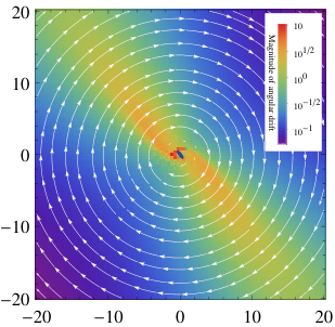

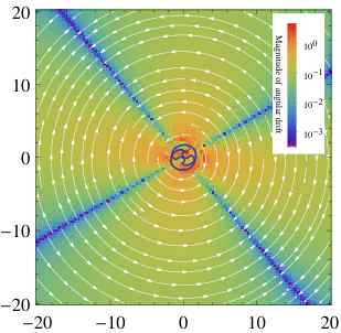

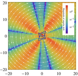

In contrast to the angular drift, the radial component of the drift field appears always to be (equally) divided into regions that are radially inwards and regions that are radially outwards. No state tested featured a radial field that was entirely radially inwards or entirely radially outwards. The simplest way in which the space may be divided is by a single dividing axis through the origin as shown in figure 1. In this case it is evident that there is as much of the space with outwards drift as there is with inwards drift. Often it is the case that two or more of these axes divide the space (see figures 2 and 3), so that the space is apportioned into wedges that alternate between flow that is radially inwards and flow that is radially outwards. In the case of two such axes (as for instance is shown in figure 2), it appears that these axes are always perpendicular, so that again half of the space exhibits inwards flow and the other half outwards flow. More complicated, bulb-like structures may sometimes be seen in the radial drift, especially in larger superpositions. To the eye however, it always appears the case that the space is equally divided into inwards and outwards regions, although a mathematical proof of whether this is indeed the case remains to be seen.
Mechanism for the relaxation of extreme quantum nonequilibrium
Any nonequilibrium distribution that is initially located away from the central region (where the Born distribution is located) cannot be considered relaxed until the vast majority of systems have at least relocated into the central region.
As discussed in the introduction, it is expected that once this happens relaxation will proceed efficiently.
It therefore becomes relevant to consider the time it takes an individual trajectory to migrate into the central region (or indeed whether this migration takes place at all).
To this end, type-1 and type-2 drift fields have a clear, identifiable mechanism by which this migration takes place.
Type-0 drift fields do not feature this mechanism. In every type-1 and type-2 field calculated, the angularly repulsive axes appear to coincide with portions of the field with inwards radial drift whilst the angularly attractive axes coincide with regions that are radially inwards. This structure is clearly displayed in figures 2 and 3. In this regard, any system that is initially separated from the bulk of the Born distribution will be swept by the dominant angular drift towards one of the angularly attractive axes. As these axes always coincide with a region of inwards radial drift, the trajectory will then be dragged into the central region where the bulk of the Born distribution is found.
In contrast to this, type-0 drift fields produce trajectories that perpetually orbit around the central region. As a trajectory does so it will sample both regions (wedges) with inwards drift and regions with outwards drift. As these appear (at least to the eye) equal in size it is tempting to conclude that, for such trajectories, outwards drift will balance inwards drift. If this were the case then trajectories would not be drawn into the central region and relaxation would not take place. Certainly it is the case that there is a balancing effect between inwards and outwards flow and so for type-0 fields relaxation from outside the central region will be at least significantly retarded if not stopped altogether. Whether or not there exists some delicate imbalance between inwards and outwards flow that eventually produces relaxation remains to be seen. An answer to this question could have important implications for studies considering conjectured quantum nonequilibrium in the early universe, and so this is clearly a direction for further work.
Although a detailed study is left for future work, the effect of the relaxation mechanism (the resulting radial transport of trajectories) is illustrated in figure 4. To produce this figure, 1000 trajectories were chosen randomly in the radial interval , and numerically evolved for 1000 wave function periods with a standard Runge-Kutta algorithm. In the first frame of the figure, the wave function parameters that produced the type-0 drift field displayed in figure 1 were used. In the second frame the wave function parameters that produced the type-1 drift field of figure 2 were used. In accordance with our statements regarding the mechanism, the type-1 drift field causes a clear inward drift of the trajectories. An ‘extreme’ quantum nonequilibrium ensemble (that is concentrated away from the central region) will therefore be transported towards the Born distribution where, as discussed, it is presumed to relax efficiently. In contrast, the type-0 drift field produces no such radial drift and, after 1000 wave function periods, the trajectories still appear close to their original radial coordinate .
Specific properties of states studied
M=3
An state has only , and components. (Or equivalently , and components.) Since the cut-off energy is , by property (xi) the total vorticity of the state may only be . Hence, there must always exist a single node with . Property (xii) ensures there is a maximum of one node and so no pair creation can take place. (The two plane algebraic curves mentioned at the end of section 2 are in this case straight lines and so intersect only once.) The sign of the vorticity may be determined with the vorticity theorem. The relevant Laurent polynomial has a simple pole at and two simple zeros at . Hence, if the vorticity is positive, else it is negative. Clearly the two possibilities appear with equal probability when wave function parameters are chosen at random. For the 100 states generated, the drift field was type-0 in every case. Hence, the relaxation of extreme nonequilibrium may be retarded for every state. The angular flow is in the direction indicated by . Note however that due to the way the are defined, should be understood to refer to positive, anticlockwise vorticity rather than the common notion of rotating to the right implied by the letter .
For the simple case, further properties of the node may be found as follows. By taking the modulus square of the state (8), the path of the node may be written (which is the general Cartesian form of a conic-section) with the coefficients
| (33) |
The condition that this path is elliptical is , which is the case unless and differ by an exact integer number of , the limiting case in which the ellipse becomes a straight line. That the ellipse is centred upon the origin is implied by the vanishing and coefficients. The nodal trajectory is circular if and , which is the case when and differ by a half-integer number of and , or equivalently . By translating the angular basis, it may be shown that the ellipse has a semi-minor axis of and a semi-major axis of . (A circular trajectory is found if either or vanish.) As the closest the node approaches the origin is , for a ground state with only perturbative contributions from and (as studied by [39]), the node stays far from the bulk of the Born distribution and interesting relaxation properties are to be expected. The orientation of the ellipse varies linearly with the difference between and . The area of the ellipse is . The nodal trajectory as a function of time may be expressed
| (34) |
M=6
By property (xi) the total vorticity may only be , or . As an state is bounded in energy by , by property (xii) there is a maximum of 4 nodes at any time. In the case of vorticity, there must always exist at least 2 nodes, each with vorticity , and one pair may create and annihilate in addition to these. All states generated with produced type-0 drift fields. In the case of , there may be zero nodes, or up to two pairs of opposite vorticity nodes. (The plane algebraic curves upon whose intersections the nodes reside are in this case conic sections which may intersect 0, 2 or 4 times.) The Vorticity 0 states produced type-1 drift fields. If the wave function parameters are chosen at random in the way described, the type-1 drift fields appear approximately 66% of the time whilst the type 0 appear approximately 17% of the time each. (The relative frequency of states was determined by randomly selecting state parameters for 100,000 states and calculating using the vorticity theorem (28).) Hence, states that exhibit retarded relaxation are relatively less common than for states, appearing in 34% of cases.
M=10
By property (xi) the total vorticity may be or , with the former possibility always featuring at least one node and the latter at least 3 nodes. In both cases property (xii), allows pair creation to increase this number up to a total of 9 nodes. The are relatively rare, each appearing in approximately 3% of randomly selected cases each. All of the 6 randomly generated states that had produced type-0 drift fields. States with each appear in approximately 47% of cases. These may exhibit any one of the three types of drift field. Of the 94 fields generated by states with , type-0 drift fields (with retarded relaxation) appeared in 7 cases, whilst type-1 and type-2 fields appeared in 72 and 15 cases respectively.
M=15
By property (xi) the total vorticity may be 0, or . States with may feature no nodes, but states with and must always retain at least 2 and 4 nodes respectively. For all possible vorticities, property (xii) and pair creation allow up to a maximum of 25 nodes. As with the superpositions, the states of maximal total vorticity are relatively rare. For superpositions, maximal vorticities each appear in approximately 0.4% of cases, whilst each appear in approximately 19% of cases. The most commonly found vorticity is , appearing in approximately 61% of cases. The single maximal vorticity state that appeared in the 100 randomly selected states produced a type-0 retarded drift field. Of the 42 random trials that had , 15 had type-0 drift fields. Of the remaining 57 trials that were found to have , not a single one produced a type-0 drift field.
Vorticity-drift conjectures
Although proofs have not been forthcoming, we advance the following statements as conjectures and argue their validity primarily on the basis of lack of counterexample.
Conjecture 1 - A state with zero total vorticity cannot produce a type-0 drift field
For sufficiently large , the velocity field of a state with zero total vorticity cannot be uniformly clockwise or uniformly anticlockwise.
To demonstrate this, consider that for a zero-vorticity state it is the case that for sufficiently large . Hence, the integrand (which is proportional to the angular component of the velocity field) must change sign or be trivially zero (in the presence of fine tuning). If, then, the drift field classifications were applied instead to velocity fields, it would be the case that zero total vorticity fields could not produce type-0 velocity fields. To support the validity of this statement when applied to drift fields, 1000 extra zero-vorticity states were generated for each of the and categories. (Property (xi) means and states cannot have zero-vorticity.) (States with maximal or zero total vorticity may be easily calculated by randomly generating many states and checking the vorticity with the vorticity theorem.) All 2000 cases were found to be type-1 or type-2, in support of the conjecture.
Conjecture 2 - All states of maximal vorticity produce type-0 drift fields
Consistently it was found that all states of maximal vorticity produced type-0 relaxation retarding states. As these states are relatively rare for and categories, however, this conjecture is certainly in need of further substantiation. To provide this, 1000 extra maximal vorticity states were generated for each of the state categories. All 4000 cases were found to be of type-0. We note that this conjecture provides a convenient method of generating these type-0 relaxation retarding states were one to wish to study their properties. One need simply to randomly generate state parameters and then check that their vorticity is maximal using the vorticity theorem.
4 Conclusions
In this paper, consideration has been given to the behaviour of de Broglie trajectories that are separated from the bulk of the Born distribution with a view to describing the quantum relaxation properties of more ‘extreme’ forms of quantum nonequilibrium. The main results are as follows. A number of new properties of nodes have been described ((vii) to (xii) in section 2) that are true under the assumption of a quantum state with bounded energy and in the absence of finely-tuned parameters. It is hoped that these results prove useful to the community and that they may be extended and generalised to suit problems other than that considered here. For the 2-dimensional isotropic oscillator (which has physical significance in studies regarding quantum nonequilibrium in the early universe [22, 28, 29, 30, 21, 31]), these properties have been shown to have consequences for the quantum relaxation of systems that are separated from the bulk of the Born distribution (what has been referred to as ‘extreme’ quantum nonequilibrium). The relaxation properties of these systems have been classified in terms of the structure of their ‘drift field’, a new concept introduced here. States have been divided into 3 distinct classes. Type-1 and type-2 drift fields have been shown to feature a mechanism that gives rise to efficient relaxation of extreme quantum nonequilibrium. Type-0 fields lack such a relaxation mechanism, appearing instead to sample the drift field in a manner that suggests the prevention of quantum relaxation. Even if it is not the case that relaxation is entirely blocked in such states, it will at least be significantly retarded. Whether or not some delicate imbalance of flow may eventually cause relaxation, and the calculation of relaxation timescales if this is indeed the case, presents a clear avenue for further investigation. Another subject that will be the focus of a future paper concerns the consequences of fine-tuning and perturbations around finely-tuned states. (In the process of this investigation, such states were found to produce highly unusual, pathological behaviour that was judged to be extraneous to the intended focus.)
For the states studied, it was found that all states of maximal total vorticity (according to their energy bound) produced type-0, relaxation-retarding drift fields. It was also found that no zero-vorticity states produced exhibit type-0 drift. In section 3 it was formally conjectured that these two correspondences are true for all (non-finely-tuned) states. These conjectures are a central result of this work which, when used with the vorticity theorem (point (x) in section 2), allow the generation of states that should exhibit efficient relaxation as well as those for which relaxation is retarded (or possibly stopped altogether). The relative abundances of these states given random parameters have been discussed. It is hoped that the identification of relaxation retarding states, and the methodology that has otherwise been formulated, may be useful to those investigating the intriguing possibility of discovering quantum nonequilibrium.
Bibliography
References
- [1] L. de Broglie. In Électrons et Photons: Rapports et Discussions du Cinquième Conseil de Physique, pages. Gauthier-Villars, Paris, 1928. [English translation in ref. [48]].
- [2] D. Bohm. A Suggested Interpretation of the Quantum Theory in Terms of “Hidden” Variables. I. Phys. Rev., 85:166–179, 1952.
- [3] D. Bohm. A Suggested Interpretation of the Quantum Theory in Terms of “Hidden” Variables. II. Phys. Rev., 85:180–193, 1952.
- [4] P. R. Holland. The Quantum Theory of Motion: an Account of the de Broglie-Bohm Causal Interpretation of Quantum Mechanics. Cambridge University Press, Cambridge, 1993.
- [5] S. Colin and W. Struyve. Quantum non-equilibrium and relaxation to equilibrium for a class of de Broglie-Bohm-type theories. New J. Phys., 12(4):043008, 2010, 0911.2823.
- [6] H. M. Wiseman. Grounding Bohmian mechanics in weak values and Bayesianism. New J. Phys., 9:165, 2007, 0706.2522.
- [7] E. Deotto and G. C. Ghirardi. Bohmian mechanics revisited. Found. Phys., 28:1–30, 1998, quant-ph/9704021.
- [8] N. G. Underwood. (In preparation). PhD thesis, Clemson University, 2018.
- [9] A. Valentini. Signal-locality, uncertainty, and the subquantum H-theorem. I. Phys. Lett. A, 156(1–2):5–11, 1991.
- [10] A. Valentini. On the Pilot-Wave Theory of Classical, Quantum and Subquantum Physics. PhD thesis, International School for Advanced Studies, Trieste, Italy, 1992.
- [11] A. Valentini and H. Westman. Dynamical origin of quantum probabilities. Proc. R. Soc. A, 461(2053):253–272, 2005, quant-ph/0403034.
- [12] M. D. Towler, N. J. Russell, and A. Valentini. Time scales for dynamical relaxation to the Born rule. Proc. R. Soc. A, 468(2140):990–1013, 2012, 1103.1589.
- [13] E. Abraham, S. Colin, and A. Valentini. Long-time relaxation in pilot-wave theory. J. Phys. A, 47(39):395306, 2014, 1310.1899.
- [14] S. Colin. Relaxation to quantum equilibrium for Dirac fermions in the de Broglie-Bohm pilot-wave theory. Proc. R. Soc. A, 468(2140):1116–1135, 2012, 1108.5496.
- [15] C. Efthymiopoulos and G. Contopoulos. Chaos in Bohmian quantum mechanics. J. Phys. A, 39:1819–1852, 2006.
- [16] D. Dürr, S. Goldstein, and N. Zanghí. Quantum equilibrium and the origin of absolute uncertainty. J. Stat. Phys., 67:843–907, 1992, quant-ph/0308039.
- [17] D. Dürr and S. Teufel. Bohmian Mechanics: The Physics and Mathematics of Quantum Theory. Springer, Berlin, 2009.
- [18] A. Valentini. In Bohmian Mechanics and Quantum Theory: An Appraisal, pages 45–66. Kluwer, Dordrecht, 1996.
- [19] A. Valentini. In Chance in Physics: Foundations and Perspectives, pages 165–181. Springer, Berlin, 2001, quant-ph/0104067.
- [20] A. Valentini. Signal-locality, uncertainty, and the subquantum H-theorem. II. Phys. Lett. A, 158(1–2):1 – 8, 1991.
- [21] N. G. Underwood and A. Valentini. Quantum field theory of relic nonequilibrium systems. Phys. Rev. D, 92(6):063531, 2015, 1409.6817.
- [22] A. Valentini. Inflationary cosmology as a probe of primordial quantum mechanics. Phys. Rev. D, 82:063513, 2010, 0805.0163.
- [23] A. Valentini. Astrophysical and cosmological tests of quantum theory. J. Phys. A, 40:3285–3303, 2007, hep-th/0610032.
- [24] A. Valentini. Black Holes, Information Loss, and Hidden Variables. 2004, hep-th/0407032.
- [25] A. Valentini. De Broglie-Bohm prediction of quantum violations for cosmological super-Hubble modes. 2008, 0804.4656.
- [26] A. Valentini. Subquantum information and computation. Pramana J. Phys., 59(2):269–277, 2002, quant-ph/0203049.
- [27] P. Pearle and A. Valentini. In Encyclopaedia of Mathematical Physics, pages 265–276. Elsevier, North-Holland, 2006, quant-ph/0506115.
- [28] S. Colin and A. Valentini. Mechanism for the suppression of quantum noise at large scales on expanding space. Phys. Rev. D, 88:103515, 2013, 1306.1579.
- [29] S. Colin and A. Valentini. Primordial quantum nonequilibrium and large-scale cosmic anomalies. Phys. Rev. D, 92(4):043520, 2015, 1407.8262.
- [30] S. Colin and A. Valentini. Robust predictions for the large-scale cosmological power deficit from primordial quantum nonequilibrium. Int. J. Mod. Phys. D, 25(06):1650068, 2016, 1510.03508.
- [31] N. G. Underwood and A. Valentini. Anomalous spectral lines and relic quantum nonequilibrium. 2016, 1609.04576.
- [32] H. Frisk. Properties of the trajectories in Bohmian mechanics. Phys. Lett. A, 227(3):139–142, 1997.
- [33] D. A. Wisniacki and E. R. Pujals. Motion of vortices implies chaos in Bohmian mechanics. EPL, 71:159–165, 2005, quant-ph/0502108.
- [34] C. Efthymiopoulos, C. Kalapotharakos, and G. Contopoulos. Nodal points and the transition from ordered to chaotic Bohmian trajectories. J. Phys. A, 40:12945–12972, 2007, 0709.2038.
- [35] A. C. Tzemos, G. Contopoulos, and C. Efthymiopoulos. Origin of chaos in 3-d Bohmian trajectories . Phys. Lett. A, 380(45):3796 – 3802, 2016, 1609.07069.
- [36] H. Wu and D. W. L. Sprung. Quantum chaos in terms of Bohm trajectories. Phys. Lett. A, 261(3–4):150 – 157, 1999.
- [37] D. A. Wisniacki, E. R. Pujals, and F. Borondo. Vortex interaction, chaos and quantum probabilities. EPL, 73:671–676, 2006, nlin/0507015.
- [38] C. Efthymiopoulos, G. Contopoulos, and A. C. Tzemos. Chaos in de Broglie-Bohm quantum mechanics and the dynamics of quantum relaxation. Annales de la Fondation Louis de Broglie, 42(133), 2017, 1703.09810.
- [39] A. Kandhadai and A. Valentini. Perturbations and quantum relaxation. 2016, 1609.04485.
- [40] P.C.W. Davies. The Physics of Time Asymmetry. University of California Press, Berkeley, 1977.
- [41] C. Cohen-Tannoudji, B. Diu, and F. Laloë. Quantum Mechanics. Wiley, 1977.
- [42] P. A. M. Dirac. Quantised singularities in the electromagnetic field,. Proc R. Soc. A, 133(821):60–72, 1931.
- [43] J. O. Hirschfelder, A. C. Christoph, and W. E. Palke. Quantum mechanical streamlines. I. Square potential barrier. J. Chem. Phys., 61(12):5435–5455, 1974.
- [44] J. O. Hirschfelder, C. J. Goebel, and L. W. Bruch. Quantized vortices around wavefunction nodes. II. J. Chem. Phys., 61(12):5456–5459, 1974.
- [45] R.E. Wyatt. Quantum Dynamics with Trajectories: Introduction to Quantum Hydrodynamics. Springer, New York, 2006.
- [46] J. O. Hirschfelder. The angular momentum, creation, and significance of quantized vortices. J. Chem. Phys., 67(12):5477–5483, 1977.
- [47] J. B. Conway. Functions of One Complex Variable. Springer-Verlag, Berlin, 1973.
- [48] G. Bacciagaluppi and A. Valentini. Quantum Theory at the Crossroads: Reconsidering the 1927 Solvay Conference. Cambridge University Press, Cambridge, 2009, quant-ph/0609184.