Particle rearrangement and softening contributions to the nonlinear mechanical response of glasses
Abstract
Amorphous materials such as metallic, polymeric, and colloidal glasses, exhibit complex preparation-dependent mechanical response to applied shear. In particular, glassy solids yield, with a mechanical response that transitions from elastic to plastic, with increasing shear strain. We perform numerical simulations to investigate the mechanical response of binary Lennard-Jones glasses undergoing athermal, quasistatic pure shear as a function of the cooling rate used to prepare them. The ensemble-averaged stress versus strain curve resembles the spatial average in the large size limit, which appears smooth and displays a putative elastic regime at small strains, a yielding-related peak in stress at intermediate strain, and a plastic flow regime at large strains. In contrast, for each glass configuration in the ensemble, the stress-strain curve consists of many short nearly linear segments that are punctuated by particle-rearrangement-induced rapid stress drops. To explain the nonlinearity of , we quantify the shape of the small stress-strain segments and the frequency and size of the stress drops in each glass configuration. We decompose the stress loss (i.e., the deviation in the slope of from that at ) into the loss from particle rearrangements and the loss from softening (i.e., the reduction of the slopes of the linear segments in ), and then compare the two contributions as a function of and . For the current studies, the rearrangement-induced stress loss is larger than the softening-induced stress loss, however, softening stress losses increase with decreasing cooling rate. We also characterize the structure of the potential energy landscape along the strain direction for glasses prepared with different , and observe a dramatic change of the properties of the landscape near the yielding transition. We then show that the rearrangement-induced energy loss per strain can serve as an order parameter for the yielding transition, which sharpens for slow cooling rates and in the large system-size limit.
pacs
62.20.-x, 63.50.Lm 64.70.kj 64.70.peI Introduction

Glass formation occurs in many different materials, spanning an enormous range of length scales, including atomic alloys, organic compounds, ceramics, and dense colloidal suspensions [1, 2]. In particular, metallic glasses have received significant attention recently for their promise in technological applications [3, 4, 5, 6] that utilize their unique combination of properties (e.g. high strength and elasticity) and processability [7, 8, 9].
Glasses are often generated by cooling a system in the liquid state sufficiently rapidly such that crystallization is avoided and the system remains disordered at low temperatures [10]. The mechanical response of glasses to applied stress is complex, including strain hardening [11], plastic yielding [12, 13, 14, 15, 16, 17], and brittle failure [18, 19, 20], and the particular response that is observed for a given glass sample depends on the protocol used to prepare and characterize it (e.g. its thermal history) [21]. The cooling rate determines the fictive temperature, at which the system falls out of metastable equilibrium [22]. The fictive temperature significantly affects mechanical properties, such as the ductility [23, 24, 25, 20, 26, 27], shear band formation [28], quality factor of vibrations [5], and the relation between stress versus strain under quasistatic compression or tension [29, 30].
The fictive temperature defines the average energy of glasses in the potential energy landscape (PEL) [31, 10], which gives the potential energy of the system as a function of all of the particle coordinates (and boundary conditions). The PEL has been used recently to describe the Gardner transition, the temperature below which the separations between basins in the landscape becomes fractal [32, 33], super-Arrhenius structural relaxation [34], as well as reversibility and memory encoding during cyclic shear in glasses [35, 36]. Studies have also quantified the width and depth of basins in the PEL using thermal activation and saddle-point identification methods [37, 38]. This prior work showed that the size of basins are smaller for more rapidly cooled glasses, while asserting that the curvature of the basins is insensitive to the cooling rate. Other computational studies have applied external shear to study the evolution of the system as the PEL deforms with strain [39, 40, 41], which strongly influences the mechanical response of glasses. Instead of focusing on small strain intervals near mechanical instabilities, in this work, we will map out the full PEL in the strain direction.
In contrast to crystalline materials, where the creation of and interaction between topological defects controls the mechanical response, it is more difficult to identify the structural defects that control the mechanical response of glasses. In glasses, strong non-affine motion in response to deformation is concentrated in “shear transformation zones” (STZs) [42, 43, 44]. Researchers have observed that particles occurring in STZs correlate with those that possess low local yield stress [45] and participate in soft modes defined from the vibrational density of states [46, 47]. These prior studies have shown that with increasing applied shear, the density of STZs increases, the elastic regions decrease in size, STZs percolate, and plastic deformation occurs [48]. Thus, rearrangements and non-affine motion in STZs also strongly impact mechanical response.
In this article, we perform computer simulations of model structural (binary Lennard-Jones) glasses undergoing athermal, quasistatic (AQS) pure shear [41] to study their mechanical response as a function of the cooling rate used to prepare them. In Fig. 1, we show the shear stress versus strain during AQS pure shear for five glass samples, all prepared at the same cooling rate. While the ensemble-averaged shear stress versus strain is smooth, the curve for each individual sample is not [49]. The left inset of Fig. 1 shows that the shear stress versus strain curve for a single configuration is composed of many nearly linear segments punctuated by stress drops over narrow strain intervals. Similar behavior occurs for the total potential energy per particle (and other quantities) versus strain, except in the case of , the segments are portions of parabolas. During the strain intervals with continuous variation of or , the system remains in a series of related minima in the PEL. At the strains corresponding to the stress drops, the system becomes unstable, particles rearrange, and the system evolves to a new lower minimum in the PEL [39, 40, 41].
Thus, it is clear that the highly nonlinear shape of the ensemble-averaged stress, potential energy, and other quantities versus strain are determined by 1) the statistics of particle rearrangements including both the frequency and size of rearrangements and 2) changes in the form of the continuous regions of the piecewise curves (i.e. softening or a decrease in the slopes of stress versus strain) between rearrangements. There have been a number of previous computational studies focusing on either particle rearrangements [23, 13, 50, 12], or softening of the shear modulus [49, 51] of binary Lennard Jones glasses under applied deformation. In this article, we will study both and compare the relative contributions from particle rearrangements and softening in determining the ensemble-averaged nonlinear mechanical response of sheared glasses as a function of the cooling rate used to prepare them.
We seek to understand the highly nonlinear behavior of the ensemble-averaged stress and potential energy versus strain (Fig. 1). Being able to explain the ensemble-averaged mechanical response is important for several reasons. First, we will show below that the system size dependence of ensemble-averaged quantities (like and ) is weak even for modest system sizes. This result suggests that the ensemble average is similar to the spatial average in the large system limit. Second, the magnitude of the particle rearrangements decreases and the frequency of particle rearrangements increases with increasing system size [12]. Thus, it becomes increasingly difficult to distinguish the continuous regions in the mechanical response from drops due to particle rearrangements in the large system limit.
As shown in Fig. 1, as the applied shear strain increases, the ensemble-averaged stress becomes nonlinear in strain, the stress reaches a peak, and then decreases to a plateau value in the large-strain limit. In the strain interval between the strain at which the slope of the stress versus strain curve begins to deviate significantly from that at zero strain and the steady-state strain regime, yielding occurs and the system transitions from an amorphous solid to a liquid-like state that can sample many different configurations. However, it is difficult to precisely define the yielding transition from the smooth, ensemble-averaged stress versus strain [52]. There are many fundamental questions concerning yielding in glasses since it involves a transition between two disordered states. For example, does yielding represent a phase transition and, if so, what is the appropriate order parameter that characterizes the transition [13]?
Recent studies of the system-size scaling of particle rearrangement statistics [13, 12], configurational overlap between minima in the PEL [14], changes in symmetry of nearest-neighbor structure [15], diffusivity of rearranging particles [16], and onset of irreversibility during cyclic shear [52, 35, 17], have suggested that yielding in glassy materials can be described as a non-equilibrium first-order phase transition. For example, the rearrangement frequency displays power-law scaling with system size, with a scaling exponent that changes strongly as the strain approaches the yield strain [13]. Beyond the yield strain, the exponent reaches a plateau value that is independent of the cooling rate. These studies have also shown that the yielding transition becomes less sharp with increasing cooling rate [13]. However, much more work is needed to fully understand the cooling-rate dependence of the rearrangement- and softening-induced losses near yielding.
We present several key results in this study. First, we show that the loss in stress from rearrangements is dominant over the softening-induced stress loss, both of which have different cooling rate and strain dependence. Second, we quantify the rearrangement- and softening-induced potential energy loss as a function of cooling rate and strain. We measure the geometric features of the basins in the PEL along the strain direction and find that the features of the PEL change dramatically near yielding. Third, we propose additional order parameters for the yielding transition based on the stress or energy loss per strain from rearrangements and softening. The stress (or energy) loss per strain increases rapidly near yielding and increasing the system size leads to a sharper transition. Finally, we calculate the distribution of energy drops from rearrangements as a function of strain for different cooling rates. We find that the distribution of energy drops is exponential with an energy scale that also changes dramatically near yielding.
The remainder of the article is organized as follows. In Sec. II, we describe the computer simulations used to prepare and shear the glasses at zero temperature, the physical quantities that will be measured during the applied shear, and the method employed to decompose the shear stress and potential energy losses into contributions from rearrangements and from softening. Sec. III presents the results from the stress and energy loss decompositions. We also characterize the geometric features of PEL basins along the strain direction. In addition, we identify quantities that change significantly with strain near yielding and assess system-size effects. In Sec. IV, we present our conclusions and describe promising future research directions concerning sheared glasses.
II methods
Our computational studies focus on model binary Lennard-Jones mixtures, which have been shown to be good glass-formers. The computer simulations are carried out in three stages: 1) Initialization of the liquid state; 2) Cooling the liquid state to a zero-temperature glass at a given rate and fixed low pressure; and 3) Application of AQS pure shear deformation at fixed low pressure.
We first perform molecular dynamics (MD) simulations of binary Lennard-Jones liquids in three dimensions under periodic boundary conditions with constant particle number and pressure . We consider large (type ) and small (type ) spherical particles by number (both with mass ) in a cubic box with volume . The particles interact pairwise via the shifted-force version of the Lennard-Jones potential, with a cutoff distance , where is the separation between particles and . The energy and length parameters follow the Kob-Andersen mixing rules [53]: , , , , , and . Length, energy, temperature, pressure, and time scales are expressed in units of , , , , and , respectively, where is Boltzmann’s constant [54]. We considered systems with , , , , and particles to study system-size effects.
To set the temperature and pressure, we incorporate a Nosé-Hoover thermostat and barostat and integrate the equations of motion using a second-order simplectic integration scheme [55, 56] with time step . We first equilibrate systems in the liquid regime at constant temperature and pressure with randomized initial particle positions and velocities. We then cool the systems into a glassy state at zero temperature using a linear cooling ramp, , over a range of cooling rates from to , all of which are above the critical cooling rate to ensure all zero-temperature samples are disordered. For each cooling rate, we consider at least configurations with random initial conditions.
After generating each zero-temperature glass, we apply AQS pure shear (AQS) at fixed pressure. For each strain step, we expand the box length and move all particles affinely in the -direction by a small strain increment and compress the box length and move all particles affinely in the -direction by the same strain increment . Following each strain step, we minimize the total enthalpy at fixed pressure , where is the total potential energy. We successively apply affine shear increments followed by potential energy minimization to a total strain . Additional details concerning the AQS pure shear algorithm can be found in our previous studies [23].
We monitor the total potential energy per particle and von Mises stress as a function of strain during the pure shear deformation. The stress tensor is given by
| (1) |
where is the component of the pairwise force that particle exerts on particle , and is the component of the center-to-center distance vector between particles and . The von Mises stress is the second invariant of the stress tensor:
| (2) |
where is the identity tensor and is the pressure [29]. We subtract the residual stress tensor from so that the von Mises stress is initialized to zero at .
As described in Sec. I, nonlinearity in ensemble-averaged quantities, such as and , is caused by particle rearrangements and changes to the forms of the piecewise segments of and between rearrangements. We analyze the relative contributions of the two effects by defining:
| (3) |
where is the stress in the absence of losses from rearrangements and softening, is the loss in stress from particle rearrangements, and is the loss in stress from softening. We define a similar expression for the total potential energy per particle:
| (4) |
where is potential energy in the absence of losses from rearrangements and softening, and and give the potential energy loss from rearrangements and softening, respectively.


In previous simulation studies of AQS pure shear [23], we developed a method to unambiguously determine whether a particle rearrangement event occurs during the strain interval to with an accuracy on the order of numerical precision. We denote the total number of rearrangements in the strain interval to as . We calculate the cumulative rearrangement-induced stress and energy loss after the rearrangements in the strain interval to as:
| (5) |
| (6) |
where indicates the strains at which rearrangements occur and and are the stress and potential energy drops at each rearrangement, respectively. (See the right inset of Fig. 1.) We also measure the rearrangement-induced stress and potential energy losses per strain:
| (7) |
| (8) |
using bins of width . The stress and potential energy losses from rearrangements ( and ), as well as the corresponding losses per strain ( and ), are shown in Fig. 2 for a single configuration prepared at .


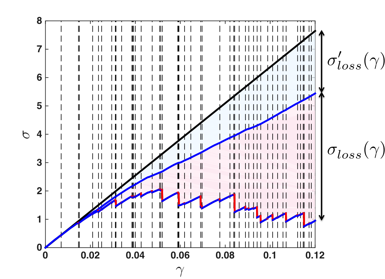
In Fig. 3, we illustrate how we quantify the effect of softening on and . In panel (a), we show for a single configuration as open circles over a small strain interval. is nearly linear in regions of strain between the three stress drops that are indicated by dashed vertical lines. We define the stress loss per strain from softening as:
| (9) |
where is the slope of in the limit (solid black line in Fig. 3 (a)) and is the slope of at strain (solid blue lines in Fig. 3 (a)). is a constant for each piecewise linear stress-strain segment and is discontinuous at rearrangements. We also measure the cumulative softening-induced stress loss for strain up to by integrating the corresponding stress loss per strain:
| (10) |
which is continuous, but the slope of the curve changes discontinuously at each rearrangement.
To quantify the effect of softening on the potential energy versus strain (Fig. 3 (b)), we find the best-fit parabola for each piecewise elastic segment between rearrangement events using
| (11) |
where , , and are coefficients that determine the concavity and location of the parabola. We define the potential energy loss per strain from softening as , where and are the local slopes of at strains and , respectively. Using Eq. 11, we define the softening-induced potential energy loss per strain as:
| (12) |
where the coefficients and are measured at . In contrast to , which is constant, depends linearly on for each inter-rearrangement segment. The cumulative softening-induced potential energy loss can be calculated by integrating over a given strain interval:
| (13) |
is piecewise quadratic, whereas is piecewise linear.
III Results
The discussion of the results is organized into three subsections. First, in Sec. 3.1, we illustrate the effects of rearrangements and softening on the ensemble-averaged stress versus strain curve as a function of the cooling rate. In particular, we compare the relative contributions of rearrangements and softening to the nonlinear mechanical response. In Sec. 3.2, we identify the distinct contributions of rearrangements and softening to the loss in potential energy as a function of strain. In addition, we study the properties of the parabolic segments of between rearrangements to characterize the width and height of basins in the PEL near the yielding transition. In Sec. 3.3, we investigate the system-size scaling exponents for the size and frequency of rearrangements and the distribution of energy drops from rearrangements near the yielding transition. In addition, we study the stress and energy losses from rearrangements and softening as a function of system size.
3.1 Stress losses from rearrangements and softening
In Fig. 4, we show the von Mises stress versus strain for a single glass configuration with prepared at undergoing AQS pure shear. We identify the elastic contribution to the stress in the absence of rearrangements and softening, the stress loss from rearrangements , and the stress loss from softening . We find that both and increase with strain. For most configurations including this one, the stress loss from rearrangements is larger than that from softening, , and the difference grows with increasing strain.
The stress loss per strain from rearrangements (Eq. 7) can be decomposed as , where is the rearrangement frequency (i.e., number of rearrangements per strain) and is the rearrangement size (i.e., stress loss per rearrangement). In Fig. 5, we show the ensemble average of all three quantities, , , and , for glasses prepared over a range of cooling rates. We find that all three increase at small strains (), plateau at large strains in the steady state regime (), and form a peak in the intermediate strain regime (). The peaks are more prominent for and . At small strains, all three quantities increase with cooling rate, indicating that rearrangements play a more significant role in stress loss in more rapidly cooled glasses. In contrast, at intermediate strains, all three quantities decrease with increasing cooling rate. In the large strain regime, none of the quantities show cooling rate dependence.
In Fig. 6 (a), we show the ensemble-averaged softening-induced stress loss per strain, (Eq. 9). increases at small strains and plateaus at cooling rate-dependent values at large strains. In the intermediate strain regime, is larger for more slowly cooled glasses with a pronounced peak. To gain insight into this behavior, we plot the ensemble-averaged slope of the continuous stress versus strain segments in Fig. 6 (b). At , the shear modulus depends on the degree of heterogeneity in the material and thus increases with decreasing [30]. As increases, decreases at small strains and reaches a plateau value () at large strains that is independent of cooling rate. In the intermediate strain regime, for slowly cooled glasses, e.g. , first decreases near and reaches a minimum near corresponding to the peak in . Thus, at small strains, the slowly cooled glasses are the most rigid, while at intermediate strains, they are the least rigid. For rapidly cooled glasses, the non-monotonic behavior in strain is absent and the shear modulus decreases continuously with strain until it plateaus in the large-strain limit.
To compare the relative contributions of rearrangements and softening on the stress loss, we integrate and over strain to obtain the cumulative stress losses, and , respectively. In Fig. 7, we show the ensemble average of the four variables in Eq. 3, as well as the direct ensemble average of stress from single glass configurations, for different cooling rates . The ensemble-averaged stress versus strain and the combination of the terms in Eq. 3, , agree quantitatively.
In general, , which means that stress losses from rearrangements are larger than those from softening. For the sake of discussion, we divide the stress versus strain curve into three regions: the pre-peak region (), the peak region (), and the post-peak region (). In the pre-peak region, the stress loss from softening is extremely small, while the stress loss from rearrangements is nonzero and increases for more rapidly cooled glasses. Significant stress loss from rearrangements in the pre-peak region for rapidly cooled glasses explains the strongly nonlinear behavior of the stress versus strain for large cooling rates . The ability of rapidly cooled glasses to undergo rearrangements in the pre-peak strain region is also correlated with enhanced ductility [23]. In the peak region, the stress loss from softening begins to grow and becomes comparable to the stress loss from rearrangements . However, and display opposite cooling rate dependence. More rapidly cooled glasses have larger stress loss from rearrangements and smaller stress loss from softening in the peak region. In contrast, more slowly cooled glasses possess smaller stress loss from rearrangements and larger stress loss from softening. In the post-peak region, both and increase linearly with . At large strains, the stress loss from rearrangements becomes cooling-rate independent. However, the cooling rate dependence of the stress loss from softening increases at large strains. In this region, increases for more slowly cooled glasses, which gives rise to the strong decay in at strains beyond the peak stress. (See Fig. 7.)
3.2 Losses in potential energy and geometric features of basins in the energy landscape
In this subsection, we will quantify the losses in the potential energy from rearrangements and softening during AQS pure shear deformation. In addition, we will characterize the geometric features of basins in the potential energy landscape along the strain direction as a function of the cooling rate used to prepare the glasses.
In Fig. 8, we show the ensemble-averaged potential energy and compare the potential energy losses from rearrangements and from softening as a function of strain. By construction, the direct ensemble-averaged potential energy agrees quantitatively with the potential energy obtained by combining the terms , , and from Eq. 4. Near , is larger for more rapidly cooled glasses since rapid cooling prevents the system from exploring configuration space and finding lower energy minima [10, 29]. At small strains, increases quadratically for all cooling rates (except for ) since the losses from rearrangements and softening are small.
As increases, the ensemble-averaged potential energy deviates from quadratic behavior due to increases in losses from rearrangements and softening . At large strains, approaches a plateau value that is independent of the cooling rate [29]. As shown in Fig. 8 (a), the potential energy loss from rearrangements increases with cooling rate for all [23]. In contrast to the behavior for the stress losses from rearrangements (Fig. 7 (a)), the potential energy loss from rearrangements is smaller than the potential energy loss from softening . In fact, at large strains, grows more rapidly with strain than . The strain dependence of originates from the evolution with strain of the geometric features of the PEL (i.e., the -dependence of the two terms, and , in Eq. 12), which will be discussed below.


As shown in Fig. 9 (a), the potential energy versus strain for a single glass configuration is composed of a series of continuous parabolic segments punctuated by rapid rearrangement-induced drops. Along the continuous segments in strain, the system remains in a series of similar minima in the potential energy landscape. As the strain continues to increase, the potential energy minimum will become unstable, the system will undergo a rearrangement and move to a new minimum. With subsequent increases in strain, the system will follow a new continuous parabolic segment until that energy minimum becomes unstable. In Fig. 9 (b), we define several geometric features of the PEL along the strain direction. For each continuous segment of , we find the best fit parabola using Eq. 11 with half-width , depth , and strain location of the minimum , where is the strain at which a rearrangement occurs (on the large strain side of the continuous segment).
In Fig. 10, we show the ensemble-averaged potential energy landscape parameters , , and as a function of strain and cooling rate . Similar to the ensemble-averaged shear modulus in Fig. 6, the concavity depends weakly on for rapidly cooled glasses. However, becomes increasingly non-monotonic in as the cooling rate decreases. In panel (b), we show that the strain location of the basin minimum occurs at at , and either increases with (for large ) or decreases with (for small ) depending on the cooling rate. Large deviations from are associated with yielding. For rapidly cooled glasses, there are many nearby minima in the PEL [57] with similar values of , , and values of that increase with strain. Thus, rapidly cooled glasses possess basins with that increase with . For more slowly cooled glasses, rearrangements below yielding are less intense (Fig. 5 (c)). In this case, changes signs and decreases with strain near yielding. As a result, for slowly cooled glasses in the strain regime near yielding. At large , for all cooling rates.
There are two contributions to the potential energy loss from softening. The first contribution, from the integration of over strain, is similar to the stress loss from softening . The second contribution stems from the integration of over . For rapidly cooled glasses, the second contribution to is larger than the first for all strains. For slowly cooled glasses, when becomes sufficiently positive near yielding (inset to Fig. 10 (b)), the second contribution can switch from positive to negative, providing an effective potential energy gain. However, for slowly cooled glasses, the potential energy loss from the first contribution is much larger than the effective gain, and thus also grows with for slowly cooled glasses as shown in Fig. 8 (a).

We now focus on the strain and cooling rate dependence of the half-width and depth of the basins that are sampled in the PEL along the strain direction during AQS pure shear. As shown in Fig. 11 (a) and (b), the ensemble-averaged and possess similar dependence on strain and cooling rate. at and then both increase with for small strains. As continues to increase, and become cooling-rate dependent. For rapidly cooled glasses, and grow monotonically with strain, reaching plateau values ( and ) in the large-strain limit. In contrast, for slowly cooled glasses, and form peaks near before reaching their large-strain plateau values. The values of for slowly cooled glasses are similar to those for the peak locations of the von Mises stress (Fig. 7 (b)), which indicates that as the strain increases above yielding, the basin geometries change dramatically.
In Fig. 11 (c), we show a scatter plot of versus for all of the continuous parabolic segments in in the range . We find that more slowly cooled glasses sample basins with larger depths and half-widths, and , as shown in the upper left inset to panel (c). At small strains, and for all cooling rates, the half-width of the basins scales quadratically with the depth, [37]. In contrast, with at large strains near and above yielding, which signifies that the dynamics has transitioned from intra-metabasin to inter-metabasin sampling [8, 58]. (See the lower right inset to panel (c).) Recent studies of unsheared, finite-temperature glasses have also shown that the basin widths and depths are larger for more slowly cooled glasses. However, these studies also showed that the basin curvature is independent of cooling rate, which differs from the results presented in Fig. 10 (a) for glasses undergoing AQS pure shear. Thus, thermal fluctuating systems and glasses undergoing AQS pure shear sample basins with different geometric properties. In summary, we have shown that the geometric properties of basins in the potential energy landscape vary strongly near yielding and depend strongly on cooling rate for glasses undergoing AQS pure shear.
3.3 Yielding transition
In this section, we analyze the system-size dependence of the stress and energy losses from rearrangements and softening. Prior studies have shown that quantities, such as the average energy drop and participation number during rearrangements, scale sublinearly with system size in glasses undergoing AQS shear [59, 12]. Other work has shown that changes in the scaling of the rearrangement statistics with system size are associated with the yielding transition [13, 17].
First, note that macroscale quantities, such as the ensemble-averaged stress and potential energy per particle , are largely independent of system size for . (See Fig. 18 in Appendix A.) In Fig 12, we show the system-size dependence of the rearrangement-induced stress loss per strain and energy loss per strain . For , and are nearly independent of system size at small and large strains. However, at strains near the yield strain , both and display sharper increases with strain as increases. For slowly cooled glasses, forms a peak near yielding (cf. Fig. 5 (c)), which persists in the large system limit. In contrast, does not possess a peak and instead displays a sigmoidal form for all cooling rates [23]. The slope of near the midpoint of the sigmoid sharpens with increasing , but reaches a (cooling-rate dependent) finite value in the large-system limit. The large-system limit for the slope of (near the midpoint) grows with decreasing cooling rate. (See Fig. 15 (a).) The rapid increase in the slope of signals a significant acceleration of rearrangements and energy loss near the yielding transition.
As described in Sec. 3.1 for , we can decompose into two contributions that give the size and frequency of rearrangements. In Fig. 13, we show the system size dependence of the ensemble average of these two quantities. As increases, the rearrangement size decreases and the frequency increases. Previous studies [13, 50, 12] have focused on the system-size scaling of similar quantities: 1) the strain interval between rearrangements and 2) the total energy loss per rearrangement .
The ensemble-averaged size and frequency of rearrangements display power-law scaling with system size:
| (14) |
| (15) |
where the scaling exponents and are functions of strain and cooling rate . In Fig 14 (a), we compare our results for with those from Ref. [13] for several cooling rates. Ref. [13] provided theoretical arguments for the strain dependence of . They argued that should jump from a nonzero, non-universal value ( for binary Lennard-Jones glasses) at to when , then jump discontinuously from zero to a nonzero value at the yield strain , and remain at a universal value as the strain increases beyond . As shown in Fig 14 (a), our data is qualitatively similar to the data for Ref. [13]. In particular, decreases from a maximal value at , remains roughly constant and small over a narrow strain interval below the yield strain, and then begins to increase beyond the yield strain, approaching a plateau value near at large strains.
The data in Fig 14 (a) suggests that decreases with decreasing cooling rate in the range , but it does not depend strongly on the cooling rate at large strains. Much larger ensemble averages should be performed to confirm these results. Using Eqs. 14 and 15, the rearrangement-induced energy loss per strain obeys . In Fig 14 (b), we show that the difference in the scaling exponents at small and large strains, while near the yield strain. A positive value for indicates that can serve as an order parameter for the yielding transition. The data for for rapidly cooled glasses with differs from that for more slowly cooled glasses. The stress and stress loss from rearrangements do not possess peaks for rapidly cooled glasses and, in this case, the yield transition behaves as a smooth crossover [13].
In Fig. 15 (b), we plot several characteristic strains (inflection points in (Fig. 8 (b)) and (Fig. 15 (a)) and the peak locations of the half-width and depth (Fig. 11 (a) and (b)) of the basins in the PEL), which are correlated with the yielding transition, as a function of cooling rate. At low cooling rates, these measures approach . As the cooling rate increases, these characteristic strains decrease. In particular, the measures of the inflection points tend to zero near . Note that and do not possess peaks for cooling rates , and thus these data points are not plotted.


The above results for the rearrangement-induced energy drops were obtained by ensemble averaging over many independent samples at each strain and cooling rate. We will now consider the distribution of energy drops as a function of strain and cooling rate. There have been a number of prior studies of the distribution of rearrangements, spanning length scales from avalanches in earthquakes and other geophysical flows [60, 61], particle rearrangements in driven granular matter [62], serrated flows in bulk metallic glasses [63], and thermally activated particle rearrangements in amorphous alloys [38]. The distribution of energy drops can display power-law scaling or exponential decay depending on the temperature and whether the driving is inertial or overdamped [64, 38, 65, 66]. For amorphous systems with AQS driving, the form of the distribution of energy drops is typically exponential [41, 50, 59].
In contrast to prior studies, we will characterize the form of the probability distribution of energy drops for each rearrangement both before and after the yielding transition. In Fig. 16, we show from rearrangements before yielding ( in panel (a)) and after yielding ( in panel (b)). Both before and after yielding, the probability distribution decays exponentially:
| (16) |
where is a function of both strain and cooling rate . Before the yielding transition, depends strongly on cooling rate, i.e. increases as the cooling rate decreases. Slowly cooled glasses have a relatively low probability for rearrangements with large before yielding. After yielding, the distribution of energy drops is only weakly dependent on cooling rate. In Fig. 16 (c), we plot the coefficient of the exponential decay of the energy drop distribution as a function of strain for several cooling rates . For more slowly cooled glasses, there is a more rapid decrease in before yielding. After yielding, is independent of and and similar to values found in related studies of rearrangements in sheared binary Lennard-Jones glasses [50, 41]. The behavior of the energy scale mirrors the behavior of the average potential energy (Fig. 8 (b)). We find that , where is a constant, and and does not depend on or . In the inset to Fig. 16 (c), we show as a function of and .
We also studied the system-size dependence of the softening-induced stress and energy losses. The softening-induced stress loss per strain is caused by decreases in the local slopes of the continuous stress versus strain segments. (See Fig. 6.) As the system size increases, the frequency of rearrangements increases (as shown in Fig. 13 (a)) and the lengths of the continuous stress versus strain segments shorten. Here, we investigate whether the local slopes of the continuous stress versus strain segments change significantly with system size.
In Fig. 17, we show for a slowly cooled glass () as a function of system size from to . is nearly independent of system size at strains prior to yielding . In contrast, at large strains above yielding, grows (and decreases) with . We see that for the larger system sizes () begins to saturate. For comparison, we show for a glass prepared at the highest cooling rate studied, . At these cooling rates, reaches a large-strain plateau value that is only weakly system-size dependent. In Appendix A, we show the system-size dependence of the softening-induced stress and energy loss per strain. Both quantities saturate in the large-system limit, with forms that are qualitatively the same as those for smaller system sizes. Thus, softening-induced losses persist in the large-system limit.
In this section, we presented results for the system-size dependence of the rearrangement- and softening-induced stress and energy losses from AQS pure shear as a function of strain and cooling rate. Several quantities (both rearrangement- and softening-induced losses) show strong system-size dependence near yielding, which serves to identify the onset of the transition from a solid-like to a flowing state. For example, the potential energy loss per strain from rearrangements shows a sigmoidal form that becomes increasingly sharp in the large-system limit and the stress loss per strain from softening shows significant system size dependence above yielding, but not below.
IV Conclusions and Future Directions
In this article, we characterized the nonlinear mechanical response of binary Lennard-Jones glasses subjected to AQS pure shear. We performed comprehensive numerical simulations as a function of strain above and below the yielding transition, cooling rates used to prepare the zero-temperature glasses over five orders of magnitude, and system sizes ranging from to .
To investigate the mechanical response, we focused on the von Mises stress and total potential energy per particle . Though it is hidden when taking an ensemble average, and for each single glass configuration are composed of continuous segments in strain punctuated by rapid drops in either stress or energy caused by particle rearrangements. Thus, deviations (typically losses) in the stress or potential energy from elastic behavior originate from two sources: 1) softening-induced losses from changes in the form of the continuous segments in strain and 2) rearrangement-induced losses that depend on the frequency and size of the energy or stress drops. A key feature of this study is that we decomposed the total stress and energy losses into contributions from both sources.
In general, both softening- and rearrangement-induced losses are small well below the yield strain, and then they begin to increase rapidly near yielding. Near and above yielding, both types of losses contribute to the nonlinear mechanical response and remain finite in the large-system limit. In the range of cooling rates studied here, rearrangement-induced stress losses are larger than softening-induced stress losses. However, the softening-induced stress losses increase with decreasing cooling rate (Fig. 7 (a)), and thus softening-induced stress losses can dominate the nonlinear mechanical response at sufficiently small cooling rates.
In many cases, the yield strain, where sheared glasses transition from a disordered solid into a flowing state, is difficult to pinpoint because many physical quantities, such as the shear stress and potential energy, vary smoothly with strain [52]. Here, we identified several quantities that show significant changes as the strain is increased above yielding. First, geometric features (i.e. the half-width and depth ) of basins in the PEL along the strain direction develop peaks near the yield strain for slowly cooled glasses. In addition, the scaling relation between the half-width and depth changes from a scaling exponent of below yielding to above yielding for all cooling rates studied. Second, the rearrangement-induced energy loss per strain possesses a sigmoidal form with a midpoint near the yield strain that becomes sharper as the cooling rate decreases and system size increases. Further, we decomposed the rearrangement-induced energy loss per strain into two terms that determine the size and frequency of rearrangements, and showed that the system-size scaling of these two terms changes near the yielding transition [13]. Third, as found previously, the distribution of energy drops decays exponentially for AQS sheared glasses over the full range of strain [41, 50, 59]. However, the energy scale of the exponential decay depends strongly on the cooling rate below yielding, while it is cooling-rate independent above yielding.
In future studies, we will investigate several key open questions. First, the current computational studies were performed using AQS pure shear [41]. How will the results we presented change when we consider glasses sheared at finite shear rate and temperature ? Suppose the timescale for structural relaxation from thermal fluctuations is given by . In the case , we expect similar results to those presented here. As the temperature increases, the system will sample higher regions of the PEL than sampled at zero temperature. The frequency of particle rearrangements will increase for as rearrangements become thermally activated instead of strain-induced mechanical instabilities [67, 68]. In future studies, we will analyze the rearrangement- and softening-induced losses at finite temperate and strain rate to determine their effects on the stress versus strain curve [49, 69], yield strain [8], and ductility [70].
Second, the computational studies presented here were performed using strain control, and thus at each strain, the system was mechanically stable with a non-zero shear modulus. In contrast, when sheared at fixed shear stress, the system will flow with zero shear modulus until the system finds a glass configuration with a shear stress that matches the applied shear stress [71, 72]. If the system cannot find a configuration that can balance the applied shear stress, the system will flow indefinitely with a well-defined average shear rate. In future studies, we will compare the rearrangement- and softening-induced stress and energy losses in the fixed shear stress and strain ensembles.
In previous computational studies, we showed that sheared frictionless granular materials, which interact via purely repulsive interactions, possess monotonic stress versus strain curves even for “slowly cooled” granular samples [73]. Based on our current results for rapidly cooled binary Lennard-Jones glasses, we expect that the stress and potential energy losses in frictionless granular materials are dominated by rearrangement-induced losses. In future studies, we will determine the relative contributions of rearrangement- and softening-induced stress and energy losses as a function of the strength and range of the attractive interactions in the interatomic potential. In particular, recent studies [74, 75] have shown that the form of the interaction potential can influence the ductility of amorphous alloys, and thus we will investigate the relative contributions of rearrangement- and softening-induced losses in ductile versus brittle glasses.
Acknowledgements.
The authors acknowledge primary financial support from NSF MRSEC DMR-1119826 (K.Z.) and partial support from NSF Grant Nos. CMMI-1462439 (C.O. and M.F.) and CMMI-1463455 (M.S.). This work was supported by the High Performance Computing facilities operated by, and the staff of, the Yale Center for Research Computing.Appendix A System-size scaling
In Figs. 7 and 8 in the main text, we showed the ensemble-averaged von Mises stress and potential energy per particle versus strain for a single system size, . In Fig. 18, we show and for system sizes ranging from to . For large , and appear to be approaching their large-system limits, although the system-size dependence at large strains is stronger than that at small strains.
In Fig. 19, we show the ensemble-averaged softening-induced stress loss per (1%) strain and energy loss per (1%) strain . For , is nearly independent of system size. Below yielding (), reaches its large-system limiting form for . In contrast, above yielding, has stronger system-size dependence, although it appears that will saturate in the large-system limit. This behavior is similar to that found for the local shear modulus in Fig. 17.
References
- [1] M. D. Ediger, C. Angell, and S. R. Nagel, J. Phys. Chem. 100, 13200 (1996).
- [2] L. Berthier and G. Biroli, Rev. Mod. Phys. 83, 587 (2011).
- [3] W. L. Johnson, MRS bulletin 24, 42 (1999).
- [4] A. Inoue and N. Nishiyama, MRS Bulletin 32, 651 (2007).
- [5] M. Kanik, P. Bordeenithikasem, G. Kumar, E. Kinser, and J. Schroers, Appl. Phys. Lett. 105, 131911 (2014).
- [6] M. Kanik, P. Bordeenithikasem, D. Kim, N. Selden, A. Desai, R. M’Closkey, and J. Schroers, Journal of Microelectromechanical Systems 24, 19 (2015).
- [7] M. Ashby and A. Greer, Scripta Mater. 54, 321 (2006).
- [8] W. Johnson and K. Samwer, Phys. Rev. Lett. 95, 195501 (2005).
- [9] J. Schroers, Phys. Today 66, 32 (2013).
- [10] P. G. Debenedetti and F. H. Stillinger, Nature 410, 259 (2001).
- [11] C. Deng and C. A. Schuh, Appl. Phys. Lett. 100, 251909 (2012).
- [12] S. Karmakar, E. Lerner, and I. Procaccia, Phys. Rev. E 82, 055103 (2010a).
- [13] H. G. E. Hentschel, P. K. Jaiswal, I. Procaccia, and S. Sastry, Phys. Rev. E 92, 062302 (2015).
- [14] P. K. Jaiswal, I. Procaccia, C. Rainone, and M. Singh, Phys. Rev. Lett. 116, 085501 (2016).
- [15] D. V. Denisov, M. T. Dang, B. Struth, A. Zaccone, G. H. Wegdam, and P. Schall, Sci. Rep. 5, 14359 (2014).
- [16] T. Kawasaki and L. Berthier, Phys. Rev. E 94, 022615 (2016).
- [17] P. Leishangthem, A. D. Parmar, and S. Sastry, Nature Commun. 8 (2017).
- [18] C. Hays, C. Kim, and W. L. Johnson, Phys. Rev. Lett. 84, 2901 (2000).
- [19] J. Lewandowski, W. Wang, and A. Greer, Philos. Mag. Lett. 85, 77 (2005).
- [20] G. Kumar, S. Prades-Rodel, A. Blatter, and J. Schroers, Scr. Mater. 65, 585 (2011).
- [21] J. Ketkaew, H. Wang, W. Chen, M. Fan, G. Pereira, Z. Liu, W. Dmowski, E. Bouchbinder, M. D. Shattuck, C. S. O’Hern, et al., “Fictive temperature controlling ductility in metallic glasses as a mechanical glass transition”, Submitted (2017).
- [22] C. T. Moynihan, A. J. Easteal, M. A. Bolt, and J. Tucker, J. Am. Ceram. Soc. 59, 12 (1976).
- [23] M. Fan, M. Wang, K. Zhang, Y. Liu, J. Schroers, M. D. Shattuck, and C. S. O’Hern, Phys. Rev. E 95, 022611 (2017).
- [24] C. H. Rycroft and E. Bouchbinder, Phys. Rev. Lett. 109, 194301 (2012).
- [25] G. Kumar, P. Neibecker, Y. H. Liu, and J. Schroers, Nature Commun. 4, 1536 (2013).
- [26] W. Li, H. Bei, Y. Tong, W. Dmowski, and Y. Gao, Appl. Phys. Lett. 103, 171910 (2013).
- [27] N. Nollmann, I. Binkowski, V. Schmidt, H. Rösner, and G. Wilde, Scr. Mater. 111, 119 (2016).
- [28] J. Zemp, M. Celino, B. Schönfeld, and J. F. Löffler, Phys. Rev. Lett. 115, 165501 (2015).
- [29] M. Utz, P. G. Debenedetti, and F. H. Stillinger, Phys. Rev. Lett. 84, 1471 (2000).
- [30] J. A., E. Bouchbinder, and I. Procaccia, Phys. Rev. E 87, 042310 (2013).
- [31] F. H. Stillinger, Science 267, 1935 (1995).
- [32] P. Charbonneau, J. Kurchan, G. Parisi, P. Urbani, and F. Zamponi, Nature Commun. 5 (2014).
- [33] C. O’Hern, Physics 9, 133 (2016).
- [34] H.-B. Yu, R. Richert, R. Maaß, and K. Samwer, Nature Commun. 6 (2015).
- [35] I. Regev, J. Weber, C. Reichhardt, K. A. Dahmen, and T. Lookman, Nature Commun. 6, 8805 (2015).
- [36] D. Fiocco, G. Foffi, and S. Sastry, Phys. Rev. Lett. 112, 025702 (2014).
- [37] Y. Fan, T. Iwashita, and T. Egami, Nature Commun. 5, 5083 (2014).
- [38] Y. Fan, T. Iwashita, and T. Egami, Phys. Rev. Lett. 115, 045501 (2015).
- [39] D. L. Malandro and D. J. Lacks, J. Chem. Phys. 110, 4593 (1999).
- [40] D. J. Lacks and M. J. Osborne, Phys. Rev. Lett. 93, 255501 (2004).
- [41] C. E. Maloney and A. Lemaître, Phys. Rev. E 74, 016118 (2006).
- [42] A. Argon and H. Kuo, Mater. Sci. Eng. 39, 101 (1979).
- [43] M. L. Falk and J. S. Langer, Phys. Rev. E 57, 7192 (1998).
- [44] J. S. Langer, Phys. Rev. E 77, 021502 (2008).
- [45] S. Patinet, D. Vandembroucq, and M. L. Falk, Phys. Rev. Lett. 117, 045501 (2016).
- [46] A. Widmer-Cooper, H. Perry, P. Harrowell, and D. R. Reichman, Nature Phys. 4, 711 (2008).
- [47] J. Ding, S. Patinet, M. L. Falk, Y. Cheng, and E. Ma, Proc. Natl. Acad. Sci. 111, 14052 (2014).
- [48] J. S. Harmon, M. D. Demetriou, W. L. Johnson, and K. Samwer, Phys. Rev. Lett. 99, 135502 (2007).
- [49] A. K. Dubey, I. Procaccia, C. A. Shor, and M. Singh, Phys. Rev. Lett. 116, 085502 (2016).
- [50] E. Lerner and I. Procaccia, Phys. Rev. E 79, 066109 (2009).
- [51] V. Chikkadi, O. Gendelman, V. Ilyin, J. Ashwin, I. Procaccia, and C. A. Shor, Europhys. Lett. 110, 48001 (2015).
- [52] I. Regev, T. Lookman, and C. Reichhardt, Phys. Rev. E 88, 062401 (2013).
- [53] W. Kob and H. C. Andersen, Phys. Rev. E 51, 4626 (1995).
- [54] M. P. Allen and D. J. Tildesley, Computer simulation of liquids (Oxford University Press, 1989).
- [55] S. Plimpton, J. Comput. Phys. 117, 1 (1995).
- [56] M. E. Tuckerman, J. Alejandre, R. López-Rendón, A. L. Jochim, and G. J. Martyna, J. Phys. A: Math. Gen. 39, 5629 (2006).
- [57] S. Büchner and A. Heuer, Phys. Rev. E 60, 6507 (1999).
- [58] C. E. Maloney and D. J. Lacks, Phys. Rev. E 73, 061106 (2006).
- [59] C. Maloney and A. Lemaître, Phys. Rev. Lett. 93, 016001 (2004).
- [60] P. Bak and C. Tang, J. Geophys. Res 94, 635 (1989).
- [61] H. Kawamura, T. Hatano, N. Kato, S. Biswas, and B. K. Chakrabarti, Rev. Mod. Phys. 84, 839 (2012).
- [62] D. Denisov, K. Lörincz, J. Uhl, K. Dahmen, and P. Schall, Nature Commun. 7 (2016).
- [63] J. Antonaglia, W. J. Wright, X. Gu, R. R. Byer, T. C. Hufnagel, M. LeBlanc, J. T. Uhl, and K. A. Dahmen, Phys. Rev. Lett. 112, 155501 (2014a).
- [64] J. Antonaglia, X. Xie, G. Schwarz, M. Wraith, J. Qiao, Y. Zhang, P. K. Liaw, J. T. Uhl, and K. A. Dahmen, Sci. Rep. 4, 4382 (2014b).
- [65] B. A. Sun, H. B. Yu, W. Jiao, H. Y. Bai, D. Q. Zhao, and W. H. Wang, Phys. Rev. Lett. 105, 35501 (2010).
- [66] K. M. Salerno, C. E. Maloney, and M. O. Robbins, Phys. Rev. Lett. 109, 105703 (2012).
- [67] A. Lemaître and C. Caroli, Phys. Rev. Lett. 103, 065501 (2009).
- [68] S. Karmakar, E. Lerner, I. Procaccia, and J. Zylberg, Phys. Rev. E 82, 031301 (2010b).
- [69] J. Rottler and M. O. Robbins, Phys. Rev. E 68, 011507 (2003).
- [70] H. B. Yu, X. Shen, Z. Wang, L. Gu, W. H. Wang, and H. Y. Bai, Phys. Rev. Lett. 108, 015504 (2012).
- [71] V. Dailidonis, V. Ilyin, P. Mishra, and I. Procaccia, Phys. Rev. E 90, 052402 (2014).
- [72] J. Lin, T. Gueudré, A. Rosso, and M. Wyart, Phys. Rev. Lett. 115, 168001 (2015).
- [73] N. Xu and C. S. O’Hern, Phys. Rev. E 73, 061303 (2006).
- [74] Y. Shi, J. Luo, F. Yuan, and L. Huang, J. Appl. Phys. 115, 043528 (2014).
- [75] O. Dauchot, S. Karmakar, I. Procaccia, and J. Zylberg, Phys. Rev. E 84, 046105 (2011).