跳到论文正文
W Papers独立论文阅读器 arXiv:1705.06320 论文正文 计算阅读时间 · 0%
引用这篇论文根据当前论文元数据生成,正式投稿前建议核对。


License: arXiv.org perpetual non-exclusive license
arXiv:1705.06320v2 [hep-ph] 01 Aug 2017

Predictive Pati-Salam theory of fermion masses and mixing

A. E. Cárcamo Hernández Affiliation: Universidad Técnica Federico Santa María
and Centro Científico-Tecnológico de Valparaíso
Casilla 110-V, Valparaíso, Chile
Email: antonio.carcamo@usm.cl
   Sergey Kovalenko Affiliation: Universidad Técnica Federico Santa María
and Centro Científico-Tecnológico de Valparaíso
Casilla 110-V, Valparaíso, Chile
Email: sergey.kovalenko@usm.cl
   José W.F. Valle Affiliation: AHEP Group, Institut de Física Corpuscular – C.S.I.C./Universitat de València, Parc Científic de Paterna.
C/ Catedrático José Beltrán, 2 E-46980 Paterna (Valencia) - SPAIN
Email: valle@ific.uv.es
   C.A. Vaquera-Araujo Affiliation: AHEP Group, Institut de Física Corpuscular – C.S.I.C./Universitat de València, Parc Científic de Paterna.
C/ Catedrático José Beltrán, 2 E-46980 Paterna (Valencia) - SPAIN
Email: vaquera@ific.uv.es
Abstract

We propose a Pati-Salam extension of the standard model incorporating a flavor symmetry based on the Δ⁡(27)\Delta\left(27\right) group. The theory realizes a realistic Froggatt-Nielsen picture of quark mixing and a predictive pattern of neutrino oscillations. We find that, for normal neutrino mass ordering, the atmospheric angle must lie in the higher octant, CP must be violated in oscillations, and there is a lower bound for the 0​ν​β​β\rm 0\nu\beta\beta decay rate. For the case of inverted mass ordering, we find that the lower atmospheric octant is preferred, and that CP can be conserved in oscillations. Neutrino masses arise from a low-scale seesaw mechanism, whose messengers can be produced by a Z′Z^{\prime} portal at the LHC.

1 Introduction

Apart from the discovery of neutrino oscillations [1, 2], no other laboratory evidence for physics beyond the standard model has been so far unambiguously confirmed. Both the origin of neutrino mass itself, as well as the understanding of the mixing pattern, require an explanation from first principles. Moreover, there is a variety of other motivations for having beyond the standard model physics [3]. One of these is the pursuit of a dynamical explanation for the origin of parity violation in the weak interaction, whose basic V-A nature is put in by hand in the formulation of the standard model. With this in mind here we propose a flavored [4, 5, 6] Pati-Salam [7] extension of the standard model, addressing both the dynamical origin of the V-A nature of the weak force, as well as the related origin of neutrino mass. In addition, as we will see, the model can shed light upon the flavor problem and make predictions. The main features of our model include:

  • •

    adequate implementation of Δ⁡(27)\Delta\left(27\right) flavor symmetry in the Pati-Salam framework and symmetry breaking

  • •

    consistent low-scale left-right symmetric seesaw mechanism for neutrinos [8, 9, 10, 11, 12]

  • •

    predictive pattern of neutrino mixing summarized in Figs. 1 and 2

  • •

    realistic pattern of quark mixing, yielding a Froggatt-Nielsen [13]-like picture of the CKM matrix

  • •

    lower bound for the 0​ν​β​β\rm 0\nu\beta\beta decay rate in Fig. 3

We note also that the model has a low-scale Z′Z^{\prime} portal through which the TeV scale messengers SaS_{a} can be pair-produced in Drell-Yan collisions at the LHC [14, 15, 16]. In addition, our model realizes a universal seesaw mechanism [17] for the down type quarks as well as the charged leptons, mediated by TeV scale exotic fermions. The latter should potentially lead to other phenomenological effects in the quark sector as well as lepton flavour violation effects.

2 The model

The model under consideration is based on the Pati-Salam gauge symmetry S​U​(4)C⊗S​U​(2)L⊗S​U​(2)RSU(4)_{C}\otimes SU\left(2\right)_{L}\otimes SU\left(2\right)_{R}, supplemented by the Δ⁡(27)⊗Z4⊗Z16\Delta\left(27\right)\otimes Z_{4}\otimes Z_{16} discrete family symmetry group. The fermion transformation properties under the Pati-Salam group are

F¯i​L\displaystyle\overline{F}_{iL} ∼(𝟒¯,𝟐,𝟏),\displaystyle\sim\left(\overline{\mathbf{4}},\mathbf{2,1}\right), Fi​R\displaystyle F_{iR} ∼(𝟒,𝟏,𝟐),\displaystyle\sim\left(\mathbf{4},\mathbf{1,2}\right), Si\displaystyle S_{i} ∼(𝟏,𝟏,𝟏),\displaystyle\sim\left(\mathbf{1},\mathbf{1,1}\right),
Ψ¯i​L\displaystyle\overline{\Psi}_{iL} ∼(𝟒¯,𝟏,𝟏),\displaystyle\sim\left(\overline{\mathbf{4}},\mathbf{1,1}\right), Ψi​R\displaystyle\Psi_{iR} ∼(𝟒,𝟏,𝟏),\displaystyle\sim\left(\mathbf{4},\mathbf{1,1}\right), i\displaystyle i =1,2,3,\displaystyle=1,2,3, (1)

where the subscript refers to fermion families. More explicitly, the standard model fermions are written in component form as

F¯i​L=(u¯i​Lu¯i​Lu¯i​Lν¯i​Ld¯i​Ld¯i​Ld¯i​Ll¯i​L)T,Fi​R=(ui​Rui​Rui​Rνi​Rdi​Rdi​Rdi​Rli​R).\overline{F}_{iL}=\left(\begin{array}[]{cccc}\overline{u}_{iL}&\overline{u}_{iL}&\overline{u}_{iL}&\overline{\nu}_{iL}\\ \overline{d}_{iL}&\overline{d}_{iL}&\overline{d}_{iL}&\overline{l}_{iL}\end{array}\right)^{T},\hskip 42.67912ptF_{iR}=\left(\begin{array}[]{cccc}u_{iR}&u_{iR}&u_{iR}&\nu_{iR}\\ d_{iR}&d_{iR}&d_{iR}&l_{iR}\end{array}\right). (2)

Notice that we have extended the fermion sector of the original Pati-Salam model [7] by introducing three fermion singlets SiS_{i}, in order to implement inverse and/or linear seesaw mechanisms for the generation of light active neutrino masses [8, 9, 10, 11, 12]. In addition, we have introduced vector-like fermions Ψ¯i​L\overline{\Psi}_{iL} and Ψi​R\Psi_{iR} so as to generate the standard model down-type quark and charged lepton masses, from a universal seesaw mechanism.

The particle content and gauge symmetry assignments are summarized in table 1.

Field F¯i​L\overline{F}_{iL} Fi​RF_{iR} Ψ¯i​L\overline{\Psi}_{iL} Ψi​R\Psi_{iR} SiS_{i} χL\chi_{L} χR\chi_{R} Φj\Phi_{j} Σ\Sigma ϕk\phi_{k} φl\varphi_{l} σ\sigma ρk\rho_{k} ηk\eta_{k} τk\tau_{k} ξk\xi_{k}
S​U​(4)CSU(4)_{C} 𝟒¯\overline{\mathbf{4}} 𝟒\mathbf{4} 𝟒¯\overline{\mathbf{4}} 𝟒\mathbf{4} 𝟏\mathbf{1} 𝟒\mathbf{4} 𝟒\mathbf{4} 𝟏\mathbf{1} 𝟏𝟓\mathbf{15} 𝟏\mathbf{1} 𝟏\mathbf{1} 𝟏\mathbf{1} 𝟏\mathbf{1} 𝟏\mathbf{1} 𝟏\mathbf{1} 𝟏\mathbf{1}
S​U​(2)LSU\left(2\right)_{L} 𝟐\mathbf{2} 𝟏\mathbf{1} 𝟏\mathbf{1} 𝟏\mathbf{1} 𝟏\mathbf{1} 𝟐\mathbf{2} 𝟏\mathbf{1} 𝟐\mathbf{2} 𝟏\mathbf{1} 𝟐\mathbf{2} 𝟏\mathbf{1} 𝟏\mathbf{1} 𝟏\mathbf{1} 𝟏\mathbf{1} 𝟏\mathbf{1} 𝟏\mathbf{1}
S​U​(2)RSU\left(2\right)_{R} 𝟏\mathbf{1} 𝟐\mathbf{2} 𝟏\mathbf{1} 𝟏\mathbf{1} 𝟏\mathbf{1} 𝟏\mathbf{1} 𝟐\mathbf{2} 𝟐\mathbf{2} 𝟏\mathbf{1} 𝟏\mathbf{1} 𝟐\mathbf{2} 𝟏\mathbf{1} 𝟏\mathbf{1} 𝟏\mathbf{1} 𝟏\mathbf{1} 𝟏\mathbf{1}
Table 1: Particle content and transformation properties under the gauge symmetry.

The fermion assignments under the flavor symmetry group Δ⁡(27)⊗Z4⊗Z16\Delta\left(27\right)\otimes Z_{4}\otimes Z_{16} are:

F¯1​L\displaystyle\overline{F}_{1L} ∼(𝟏𝟎,𝟎,1,i),\displaystyle\sim\left(\mathbf{1}_{\mathbf{0,0}},1,i\right), F¯2​L\displaystyle\overline{F}_{2L} ∼(𝟏𝟐,𝟎,i,i12),\displaystyle\sim\left(\mathbf{1}_{\mathbf{2,0}},i,i^{\frac{1}{2}}\right), F¯3​L\displaystyle\overline{F}_{3L} ∼(𝟏𝟏,𝟎,1,1),\displaystyle\sim\left(\mathbf{1}_{\mathbf{1,0}},1,1\right),
F1​R\displaystyle F_{1R} ∼(𝟏𝟎,𝟎,1,i),\displaystyle\sim\left(\mathbf{1}_{\mathbf{0,0}},1,i\right), F2​R\displaystyle F_{2R} ∼(𝟏𝟏,𝟎,i,i12),\displaystyle\sim\left(\mathbf{1}_{\mathbf{1,0}},i,i^{\frac{1}{2}}\right), F3​R\displaystyle F_{3R} ∼(𝟏𝟐,𝟎,1,1),\displaystyle\sim\left(\mathbf{1}_{\mathbf{2,0}},1,1\right),
Ψ¯1​L\displaystyle\overline{\Psi}_{1L} ∼(𝟏𝟎,𝟎,1,1)\displaystyle\sim\left(\mathbf{1}_{\mathbf{0,0}},1,1\right) Ψ¯2​L\displaystyle\overline{\Psi}_{2L} ∼(𝟏𝟐,𝟎,1,1),\displaystyle\sim\left(\mathbf{1}_{\mathbf{2,0}},1,1\right), Ψ¯3​L\displaystyle\overline{\Psi}_{3L} ∼(𝟏𝟏,𝟎,1,1)\displaystyle\sim\left(\mathbf{1}_{\mathbf{1,0}},1,1\right)
Ψ1​R\displaystyle\Psi_{1R} ∼(𝟏𝟎,𝟎,1,1),\displaystyle\sim\left(\mathbf{1}_{\mathbf{0,0}},1,1\right), Ψ2​R\displaystyle\Psi_{2R} ∼(𝟏𝟏,𝟎,1,1),\displaystyle\sim\left(\mathbf{1}_{\mathbf{1,0}},1,1\right), Ψ3​R\displaystyle\Psi_{3R} ∼(𝟏𝟐,𝟎,1,1),\displaystyle\sim\left(\mathbf{1}_{\mathbf{2,0}},1,1\right),
S\displaystyle S ∼(𝟑,i,1),\displaystyle\sim\left(\mathbf{3,}i,1\right), (3)

where the numbers in boldface stand for the dimensions of the Δ⁡(27)\Delta\left(27\right) irreducible representations, and we have defined S≡(S1,S2,S3)S\equiv\left(S_{1},S_{2},S_{3}\right). Notice that the three Pati-Salam singlet fermions are grouped into a Δ⁡(27)\Delta\left(27\right) triplet SS, whereas the remaining fermions are assigned to singlet representations of Δ⁡(27)\Delta\left(27\right). These fermion flavor symmetry transformation properties are summarized in table 2. A brief summary of the properties of Δ⁡(27)\Delta\left(27\right) group and its irreducible representations is given in Appendix A.

Field F¯1​L\overline{F}_{1L} F¯2​L\overline{F}_{2L} F¯3​L\overline{F}_{3L} F1​RF_{1R} F2​RF_{2R} F3​RF_{3R} Ψ¯1​L\overline{\Psi}_{1L} Ψ¯2​L\overline{\Psi}_{2L} Ψ¯3​L\overline{\Psi}_{3L} Ψ1​R\Psi_{1R} Ψ2​R\Psi_{2R} Ψ3​R\Psi_{3R} SS
Δ⁡(27)\Delta(27) 𝟏𝟎,𝟎\mathbf{1}_{\mathbf{0,0}} 𝟏𝟐,𝟎\mathbf{1}_{\mathbf{2,0}} 𝟏𝟏,𝟎\mathbf{1}_{\mathbf{1,0}} 𝟏𝟎,𝟎\mathbf{1}_{\mathbf{0,0}} 𝟏𝟏,𝟎\mathbf{1}_{\mathbf{1,0}} 𝟏𝟐,𝟎\mathbf{1}_{\mathbf{2,0}} 𝟏𝟎,𝟎\mathbf{1}_{\mathbf{0,0}} 𝟏𝟐,𝟎\mathbf{1}_{\mathbf{2,0}} 𝟏𝟏,𝟎\mathbf{1}_{\mathbf{1,0}} 𝟏𝟎,𝟎\mathbf{1}_{\mathbf{0,0}} 𝟏𝟏,𝟎\mathbf{1}_{\mathbf{1,0}} 𝟏𝟐,𝟎\mathbf{1}_{\mathbf{2,0}} 𝟑\mathbf{3}
Z4Z_{4} 11 ii 11 11 ii 11 11 11 11 11 11 11 ii
Z16Z_{16} ii i12i^{\frac{1}{2}} 11 ii i12i^{\frac{1}{2}} 11 11 11 11 11 11 11 11
Table 2: Transformation properties of the leptons and quarks under the flavor symmetry Δ⁡(27)⊗Z4⊗Z4′\Delta(27)\otimes Z_{4}\otimes Z_{4}^{\prime}.

We now turn to the main features of the scalar sector. The Higgs fields of the model are assumed to transform under the Pati-Salam gauge group as

χR\displaystyle\chi_{R} ∼(𝟒,𝟏,𝟐),\displaystyle\sim\left(\mathbf{4},\mathbf{1,2}\right), χL\displaystyle\chi_{L} ∼(𝟒,𝟐,𝟏),\displaystyle\sim\left(\mathbf{4},\mathbf{2,1}\right), Φj\displaystyle\Phi_{j} ∼(𝟏,𝟐,𝟐),\displaystyle\sim\left(\mathbf{1},\mathbf{2,2}\right), Σ\displaystyle\Sigma ∼(𝟏𝟓,𝟏,𝟏),\displaystyle\sim\left(\mathbf{15},\mathbf{1,1}\right), j\displaystyle j =1,2,\displaystyle=1,2,
ϕk\displaystyle\phi_{k} ∼(𝟏,𝟐,𝟏),\displaystyle\sim\left(\mathbf{1},\mathbf{2,1}\right), φl\displaystyle\varphi_{l} ∼(𝟏,𝟏,𝟐),\displaystyle\sim\left(\mathbf{1},\mathbf{1,2}\right), σ\displaystyle\sigma ∼(𝟏,𝟏,𝟏),\displaystyle\sim\left(\mathbf{1},\mathbf{1,1}\right), ρk\displaystyle\rho_{k} ∼(𝟏,𝟏,𝟏),\displaystyle\sim\left(\mathbf{1},\mathbf{1,1}\right), l\displaystyle l =1,2,3,4,5,\displaystyle=1,2,3,4,5,
ηk\displaystyle\eta_{k} ∼(𝟏,𝟏,𝟏),\displaystyle\sim\left(\mathbf{1},\mathbf{1,1}\right), τk\displaystyle\tau_{k} ∼(𝟏,𝟏,𝟏),\displaystyle\sim\left(\mathbf{1},\mathbf{1,1}\right), ξk\displaystyle\xi_{k} ∼(𝟏,𝟏,𝟏),\displaystyle\sim\left(\mathbf{1},\mathbf{1,1}\right), k\displaystyle k =1,2,3,\displaystyle=1,2,3, (4)

and the scalars χL,R\chi_{L,R}, Φk\Phi_{k} and Σ\Sigma develop vacuum expectation values (VEVs) of the form

⟨χL,R⟩=(000vL,R0000),⟨Φj⟩=(v1(j)00v2(j)),⟨Σ⟩=vΣ​T15,\left\langle\chi_{L,R}\right\rangle=\left(\begin{array}[]{cccc}0&0&0&v_{L,R}\\ 0&0&0&0\end{array}\right),\hskip 42.67912pt\left\langle\Phi_{j}\right\rangle=\left(\begin{array}[]{cc}v_{1}^{\left(j\right)}&0\\ 0&v_{2}^{\left(j\right)}\end{array}\right),\hskip 42.67912pt\left\langle\Sigma\right\rangle=v_{\Sigma}T^{15}, (5)

with T15=12​6​diag​(1,1,1,−3)T^{15}=\frac{1}{2\sqrt{6}}\mathrm{diag}\left(1,1,1,-3\right).

The transformation properties of the scalar fields under the Δ⁡(27)⊗Z4⊗Z16\Delta\left(27\right)\otimes Z_{4}\otimes Z_{16} discrete group are given as follows:

χR\displaystyle\chi_{R} ∼(𝟏𝟎,𝟎,i,1),\displaystyle\sim\left(\mathbf{1}_{\mathbf{0,0}}\mathbf{,}i,1\right), χL\displaystyle\chi_{L} ∼(𝟏𝟎,𝟎,−i,1),\displaystyle\sim\left(\mathbf{1}_{\mathbf{0,0}}\mathbf{,-}i,1\right), Φ1\displaystyle\Phi_{1} ∼(𝟏𝟎,𝟎,1,1),\displaystyle\sim\left(\mathbf{1}_{\mathbf{0,0}},1,1\right), Φ2\displaystyle\Phi_{2} ∼(𝟏𝟎,𝟎,−1,1),\displaystyle\sim\left(\mathbf{1}_{\mathbf{0,0}},-1,1\right),
Σ\displaystyle\Sigma ∼(𝟏𝟎,𝟎,1,e3​π​i4),\displaystyle\sim\left(\mathbf{1}_{\mathbf{0,0}},1,e^{\frac{3\pi i}{4}}\right), ϕ1\displaystyle\phi_{1} ∼(𝟏𝟎,𝟎,1,e−2​π​i8),\displaystyle\sim\left(\mathbf{1}_{\mathbf{0,0}},1,e^{-\frac{2\pi i}{8}}\right), ϕ2\displaystyle\phi_{2} ∼(𝟏𝟎,𝟎,−i,e−π​i8),\displaystyle\sim\left(\mathbf{1}_{\mathbf{0,0}},-i,e^{-\frac{\pi i}{8}}\right), ϕ3\displaystyle\phi_{3} ∼(𝟏𝟎,𝟎,1,1),\displaystyle\sim\left(\mathbf{1}_{\mathbf{0,0}},1,1\right),
φ1\displaystyle\varphi_{1} ∼(𝟏𝟎,𝟎,1,e−2​π​i8),\displaystyle\sim\left(\mathbf{1}_{\mathbf{0,0}},1,e^{-\frac{2\pi i}{8}}\right), φ2\displaystyle\varphi_{2} ∼(𝟏𝟎,𝟎,−i,e−π​i8),\displaystyle\sim\left(\mathbf{1}_{\mathbf{0,0}},-i,e^{-\frac{\pi i}{8}}\right), φ3\displaystyle\varphi_{3} ∼(𝟏𝟎,𝟎,1,1),\displaystyle\sim\left(\mathbf{1}_{\mathbf{0,0}},1,1\right), φ4\displaystyle\varphi_{4} ∼(𝟏𝟐,𝟎,−i,e−π​i8),\displaystyle\sim\left(\mathbf{1}_{\mathbf{2,0}},-i,e^{-\frac{\pi i}{8}}\right),
φ5\displaystyle\varphi_{5} ∼(𝟏𝟐,𝟎,1,eπ​i8),\displaystyle\sim\left(\mathbf{1}_{\mathbf{2,0}},1,e^{\frac{\pi i}{8}}\right), σ\displaystyle\sigma ∼(𝟏𝟎,𝟎,1,e−π​i8),\displaystyle\sim\left(\mathbf{1}_{\mathbf{0,0}},1,e^{-\frac{\pi i}{8}}\right), ρ\displaystyle\rho ∼(𝟑¯,1,i)\displaystyle\sim\left(\overline{\mathbf{3}},1,i\right) η\displaystyle\eta ∼(𝟑¯,−i,i12),\displaystyle\sim\left(\overline{\mathbf{3}},-i,i^{\frac{1}{2}}\right),
τ\displaystyle\tau ∼(𝟑¯,1,1),\displaystyle\sim\left(\overline{\mathbf{3}},1,1\right), ξ\displaystyle\xi ∼(𝟑¯,−1,1)\displaystyle\sim\left(\overline{\mathbf{3}},-1,1\right) (6)

where we have set

ρ\displaystyle\rho ≡(ρ1,ρ2,ρ3)\displaystyle\equiv\left(\rho_{1},\rho_{2},\rho_{3}\right) η\displaystyle\eta =(η1,η2,η3)\displaystyle=\left(\eta_{1},\eta_{2},\eta_{3}\right) τ\displaystyle\tau ≡(τ1,τ2,τ3)\displaystyle\equiv\left(\tau_{1},\tau_{2},\tau_{3}\right) ξ\displaystyle\xi ≡(ξ1,ξ2,ξ3).\displaystyle\equiv\left(\xi_{1},\xi_{2},\xi_{3}\right). (7)

These flavor symmetry scalar transformation properties are summarized in table 3.

Field χL\chi_{L} χR\chi_{R} Φ1\Phi_{1} Φ2\Phi_{2} Σ\Sigma ϕ1\phi_{1} ϕ2\phi_{2} ϕ3\phi_{3} φ1\varphi_{1} φ2\varphi_{2} φ3\varphi_{3} φ4\varphi_{4} φ5\varphi_{5} σ\sigma ρ\rho η\eta τ\tau ξ\xi
Δ⁡(27)\Delta(27) 𝟏𝟎,𝟎\mathbf{1}_{\mathbf{0,0}} 𝟏𝟎,𝟎\mathbf{1}_{\mathbf{0,0}} 𝟏𝟎,𝟎\mathbf{1}_{\mathbf{0,0}} 𝟏𝟎,𝟎\mathbf{1}_{\mathbf{0,0}} 𝟏𝟎,𝟎\mathbf{1}_{\mathbf{0,0}} 𝟏𝟎,𝟎\mathbf{1}_{\mathbf{0,0}} 𝟏𝟎,𝟎\mathbf{1}_{\mathbf{0,0}} 𝟏𝟎,𝟎\mathbf{1}_{\mathbf{0,0}} 𝟏𝟎,𝟎\mathbf{1}_{\mathbf{0,0}} 𝟏𝟎,𝟎\mathbf{1}_{\mathbf{0,0}} 𝟏𝟎,𝟎\mathbf{1}_{\mathbf{0,0}} 𝟏𝟐,𝟎\mathbf{1}_{\mathbf{2,0}} 𝟏𝟐,𝟎\mathbf{1}_{\mathbf{2,0}} 𝟏𝟎,𝟎\mathbf{1}_{\mathbf{0,0}} 𝟑¯\overline{\mathbf{3}} 𝟑¯\overline{\mathbf{3}} 𝟑¯\overline{\mathbf{3}} 𝟑¯\overline{\mathbf{3}}
Z4Z_{4} −i-i ii 11 −1-1 11 11 −i-i 11 11 −i-i 11 −i-i 11 11 11 −i-i 11 −1-1
Z16Z_{16} 11 11 11 11 i32i^{\frac{3}{2}} i−12i^{-\frac{1}{2}} i−14i^{-\frac{1}{4}} 11 i−12i^{-\frac{1}{2}} i−14i^{-\frac{1}{4}} 11 i−14i^{-\frac{1}{4}} i14i^{\frac{1}{4}} i−14i^{-\frac{1}{4}} ii i12i^{\frac{1}{2}} 11 11
Table 3: Transformation properties of the scalars under the flavor symmetry Δ⁡(27)⊗Z4⊗Z4′\Delta(27)\otimes Z_{4}\otimes Z_{4}^{\prime}.

With the above particle content and transformation properties the following relevant Yukawa terms arise:

−ℒY\displaystyle-\mathcal{L}_{Y} =\displaystyle= y1​F¯1​L​Φ1​F1​R​σ8Λ8+y2​F¯2​L​Φ2​F2​R​σ4Λ4+y3​F¯3​L​Φ1​F3​R\displaystyle y_{1}\overline{F}_{1L}\Phi_{1}F_{1R}\frac{\sigma^{8}}{\Lambda^{8}}+y_{2}\overline{F}_{2L}\Phi_{2}F_{2R}\frac{\sigma^{4}}{\Lambda^{4}}+y_{3}\overline{F}_{3L}\Phi_{1}F_{3R} (8)
+α1Λ​F¯1​L​χL​(S​ρ)𝟏𝟎,𝟎​σ8Λ8+α2Λ​F¯2​L​χL​(S​η)𝟏𝟏,𝟎​σ4Λ4+α3Λ​F¯3​L​χL​(S​τ)𝟏𝟐,𝟎\displaystyle+\frac{\alpha_{1}}{\Lambda}\overline{F}_{1L}\chi_{L}\left(S\rho\right)_{\mathbf{1}_{\mathbf{0,0}}}\frac{\sigma^{8}}{\Lambda^{8}}+\frac{\alpha_{2}}{\Lambda}\overline{F}_{2L}\chi_{L}\left(S\eta\right)_{\mathbf{1}_{\mathbf{1,0}}}\frac{\sigma^{4}}{\Lambda^{4}}+\frac{\alpha_{3}}{\Lambda}\overline{F}_{3L}\chi_{L}\left(S\tau\right)_{\mathbf{1}_{\mathbf{2,0}}}
+β1Λ​F1​R​χR†​(S​ρ)𝟏𝟎,𝟎​σ8Λ8+β2Λ​F2​R​χR†​(S​η)𝟏𝟐,𝟎​σ4Λ4+β3Λ​F3​R​χR†​(S​τ)𝟏𝟏,𝟎\displaystyle+\frac{\beta_{1}}{\Lambda}F_{1R}\chi_{R}^{\dagger}\left(S\rho\right)_{\mathbf{1}_{\mathbf{0,0}}}\frac{\sigma^{8}}{\Lambda^{8}}+\frac{\beta_{2}}{\Lambda}F_{2R}\chi_{R}^{\dagger}\left(S\eta\right)_{\mathbf{1}_{\mathbf{2,0}}}\frac{\sigma^{4}}{\Lambda^{4}}+\frac{\beta_{3}}{\Lambda}F_{3R}\chi_{R}^{\dagger}\left(S\tau\right)_{\mathbf{1}_{\mathbf{1,0}}}
+κ1​F¯1​L​ϕ1​Ψ1​R​σ2Λ2+κ2​F¯2​L​ϕ2​Ψ2​R​σΛ+κ3​F¯3​L​ϕ3​Ψ3​R\displaystyle+\kappa_{1}\overline{F}_{1L}\phi_{1}\Psi_{1R}\frac{\sigma^{2}}{\Lambda^{2}}+\kappa_{2}\overline{F}_{2L}\phi_{2}\Psi_{2R}\frac{\sigma}{\Lambda}+\kappa_{3}\overline{F}_{3L}\phi_{3}\Psi_{3R}
+γ1​Ψ¯1​L​φ1​F1​R​σ2Λ2+γ2​Ψ¯2​L​φ2​F2​R​σΛ+γ3​Ψ¯3​L​φ3​F3​R\displaystyle+\gamma_{1}\overline{\Psi}_{1L}\varphi_{1}F_{1R}\frac{\sigma^{2}}{\Lambda^{2}}+\gamma_{2}\overline{\Psi}_{2L}\varphi_{2}F_{2R}\frac{\sigma}{\Lambda}+\gamma_{3}\overline{\Psi}_{3L}\varphi_{3}F_{3R}
+γ4​Ψ¯1​L​φ4​F2​R​σΛ+γ5​Ψ¯1​L​φ5∗​F3​R​σ∗Λ+γ6​Ψ¯2​L​φ5​F3​R​σΛ\displaystyle+\gamma_{4}\overline{\Psi}_{1L}\varphi_{4}F_{2R}\frac{\sigma}{\Lambda}+\gamma_{5}\overline{\Psi}_{1L}\varphi_{5}^{\ast}F_{3R}\frac{\sigma^{\ast}}{\Lambda}+\gamma_{6}\overline{\Psi}_{2L}\varphi_{5}F_{3R}\frac{\sigma}{\Lambda}
+∑i=13[AiΨ¯i​LΨi​R+aiΨ¯r​i​L(Σ)srΨi​Rsσ6Λ6]+λ1(S¯SC)𝟑S1ξ+λ2(S¯SC)𝟑S2ξ+h.c.,\displaystyle+\sum\limits_{i=1}^{3}\left[A_{i}\overline{\Psi}_{iL}\Psi_{iR}+a_{i}\overline{\Psi}_{riL}\left(\Sigma\right)_{s}^{r}\Psi_{iR}^{s}\frac{\sigma^{6}}{\Lambda^{6}}\right]+\lambda_{1}\left(\overline{S}S^{C}\right)_{\mathbf{3}_{S_{1}}}\xi+\lambda_{2}\left(\overline{S}S^{C}\right)_{\mathbf{3}_{S_{2}}}\xi+\mathrm{h.c.},

where rr, ss are S​U​(4)SU\left(4\right) indices and yiy_{i}, αi\alpha_{i}, βi\beta_{i}, κi\kappa_{i}, aia_{i} (i=1,2,3i=1,2,3), γm\gamma_{m} (m=1,2,⋯,6m=1,2,\cdots,6) and λj\lambda_{j} (j=1,2j=1,2) are 𝒪⁡(1)\mathcal{O}(1) dimensionless couplings. For an explanation of the Δ⁡(27)\Delta(27) notation used in the α,β\alpha,\beta and λ\lambda-terms, see Appendix A. It is noteworthy that the lightest of the physical neutral scalar states of (Φj)11\left(\Phi_{j}\right)_{11}, (Φj)22\left(\Phi_{j}\right)_{22}, ϕi\phi_{i} should be interpreted as the SM-like 125 GeV Higgs recently found at the LHC. Furthermore, our model at low energies corresponds to a seven Higgs doublet model with five scalar singlets (these scalar singlets come from φl\varphi_{l}). As we will show in section 4, the top quark mass only arises from (Φ1)11\left(\Phi_{1}\right)_{11}. Consequently, the dominant contribution to the SM-like 125 GeV Higgs mainly arises from (Φ1)11\left(\Phi_{1}\right)_{11}. We note also that the scalar potential of our model has many free parameters, so that we can assume the remaining scalars to be heavy and outside the LHC reach. Moreover, one can suppress the loop effects of the heavy scalars contributing to precision observables, by making an appropriate choice of the free parameters in the scalar potential. These adjustments do not affect the physical observables in the quark and lepton sectors, which are determined mainly by the Yukawa couplings.

The full symmetry group 𝒢\mathcal{G} exhibits the following spontaneous breaking pattern:

𝒢=S​U​(4)C⊗S​U​(2)L⊗S​U​(2)R⊗Δ⁡(27)⊗Z4⊗Z16\displaystyle\mathcal{G}=SU(4)_{C}\otimes SU\left(2\right)_{L}\otimes SU\left(2\right)_{R}\otimes\Delta\left(27\right)\otimes Z_{4}\otimes Z_{16} (9)
⟨Σ⟩∼ΛP​S\displaystyle\langle\Sigma\rangle\sim\Lambda_{PS}
⇓\displaystyle\Downarrow
S​U​(3)C⊗S​U​(2)L⊗S​U​(2)R⊗U​(1)B−L\displaystyle SU(3)_{C}\otimes SU\left(2\right)_{L}\otimes SU\left(2\right)_{R}\otimes U\left(1\right)_{B-L} (10)
⟨χR⟩∼vR\displaystyle\langle\chi_{R}\rangle\sim\ v_{R}\ \
⇓\displaystyle\Downarrow
S​U​(3)C⊗S​U​(2)L⊗U​(1)Y\displaystyle SU(3)_{C}\otimes SU\left(2\right)_{L}\otimes U\left(1\right)_{Y} (11)
⟨Φ1,2⟩∼v\displaystyle\langle\Phi_{{1,2}}\rangle\sim\ v\ \ \ \
⇓\displaystyle\Downarrow
S​U​(3)C⊗U​(1)Q.\displaystyle SU(3)_{C}\otimes U\left(1\right)_{Q}. (12)

Here v=246v=246 GeV is the electroweak symmetry breaking scale, and we assume that the Pati-Salam gauge symmetry is broken at the scale ΛP​S ∼ ∼>106\Lambda_{PS}\mathrel{\hbox to0.0pt{\lower 4.0pt\hbox{\hskip 1.0pt$\sim$}\hss}\raise 1.0pt\hbox{$\mathrel{\hbox to0.0pt{\lower 4.0pt\hbox{\hskip 1.0pt$\sim$}\hss}\raise 1.0pt\hbox{$>$}}$}}10^{6} GeV. This restriction follows from the experimental limit on the branching ratio for the rare neutral meson decays, such as B0→li±​lj∓B^{0}\to l_{i}^{\pm}l_{j}^{\mp}, mediated by the vector leptoquarks, as discussed in Refs. [18, 19]. Furthermore, it is worth mentioning that Pati-Salam models with a quark-lepton unification scale of about  ∼>106\mathrel{\hbox to0.0pt{\lower 4.0pt\hbox{\hskip 1.0pt$\sim$}\hss}\raise 1.0pt\hbox{$>$}}10^{6} GeV can fulfill gauge coupling unification [20]. A comprehensive study of gauge coupling unification in models that include all possible chains of Pati-Salam symmetry breaking in both supersymmetric and non-supersymmetric scenarios has been given in Ref. [20].

3 Understanding the model setup

In this section we try to motivate in more detail our choice for the model content and the transformation properties. First note that the Pati-Salam gauge symmetry S​U​(4)C⊗S​U​(2)L⊗S​U​(2)RSU(4)_{C}\otimes SU\left(2\right)_{L}\otimes SU\left(2\right)_{R} breaks down to the conventional left-right symmetry S​U​(3)C⊗S​U​(2)L⊗S​U​(2)R⊗U​(1)B−LSU(3)_{C}\otimes SU\left(2\right)_{L}\otimes SU\left(2\right)_{R}\otimes U\left(1\right)_{B-L} by the VEV of the scalar field Σ\Sigma, at the scale ΛP​S ∼>106\Lambda_{PS}\mathrel{\hbox to0.0pt{\lower 4.0pt\hbox{\hskip 1.0pt$\sim$}\hss}\raise 1.0pt\hbox{$>$}}10^{6} GeV. The next symmetry breaking step is triggered by χR\chi_{R}, whose VEV is assumed to be in the few TeV scale, playing an important role in implementing the low-scale seesaw neutrino mass generation [9, 10]. The breaking of the electroweak gauge group S​U​(3)C⊗S​U​(2)L⊗U​(1)YSU(3)_{C}\otimes SU\left(2\right)_{L}\otimes U\left(1\right)_{Y} is triggered by the scalar fields Φj\Phi_{j}, which acquire vacuum expectation values at the electroweak symmetry breaking scale v=246v=246 GeV.

Besides, note that the presence of the scalar field Σ\Sigma transforming as the adjoint representation of S​U​(4)SU\left(4\right) is also crucial in the implementation of the Universal Seesaw mechanism for down-type quarks and charged leptons, mediated by exotic fermions. This scalar field Σ\Sigma acquires a VEV at the scale ΛP​S\Lambda_{PS}, so that an insertion σ6Λ6\frac{\sigma^{6}}{\Lambda^{6}} in its corresponding Yukawa term generates a TeV scale contribution to the exotic charged lepton and exotic down-type quark masses. The charge of Σ\Sigma under the Z16Z_{16} discrete group ensures that its different contributions to the charged leptons and down type quark masses will be comparable to the ones arising from the Ai​Ψ¯i​L​Ψi​RA_{i}\overline{\Psi}_{iL}\Psi_{iR} (i=1,2,3i=1,2,3) mass terms (which contribute equally to the down type quark and charged lepton masses). It is worth mentioning that we are assuming Ai≈𝒪⁡(1)A_{i}\approx\mathcal{O}(1) TeV. Let us note that the inclusion of the scalar field Σ\Sigma is necessary to guarantee that the resulting down-type quark masses are different from the charged lepton masses, as it will be shown in Section 4.

Notice that the scalars ϕi\phi_{i} and φl\varphi_{l} are needed to generate the mixing between the standard model charged leptons and down-type quarks with their exotic siblings, so as to implement the Universal Seesaw mechanism that gives rise to realistic masses for the standard model charged fermions. The scalar fields χR,χL\chi_{R},\chi_{L} and ξi\xi_{i} have Yukawa terms necessary for the implementation of the inverse and linear seesaw mechanisms, so as to generate the light active neutrino masses. This requires also that VEVs of ξi\xi_{i} are much smaller than the electroweak symmetry breaking scale.

The scalar fields ρi\rho_{i} , ηi\eta_{i} and τi\tau_{i} are needed to generate the diagonal 3×33\times 3 blocks that include the mixing of the neutrino states contained in F¯i​L\overline{F}_{iL} and Fi​RF_{iR} with the singlet neutrinos SiS_{i} (i=1,2,3i=1,2,3), thus avoiding the transmission of the strong hierarchy in the up mass matrix to the light active neutrino mass matrix. Furthermore, the scalar field σ\sigma, charged under the Z16Z_{16} discrete group is need to generate the observed SM charged fermion mass and quark mixing hierarchy. In order to relate the quark masses with the quark mixing parameters, we assume that the scalar field σ\sigma acquires a VEV equal to λ​Λ\lambda\Lambda, where λ=0.225\lambda=0.225 is one of the Wolfenstein parameters and Λ\Lambda is the cutoff of our model. In summary, the set of VEVs of the scalar fields is assumed to satisfy the following hierarchy:

vL≪vξ≪v1(j)∼vϕi∼vφl∼v≪vR≪vρ=vη=vτ∼ΛP​S∼vσ=λ​Λ,v_{L}\ll v_{\xi}\ll v_{1}^{\left(j\right)}\sim v_{\phi_{i}}\sim v_{\varphi_{l}}\sim v\ll v_{R}\ll v_{\rho}=v_{\eta}=v_{\tau}\sim\Lambda_{PS}\sim v_{\sigma}=\lambda\Lambda, (13)

where ⟨χL,R⟩=vL,R\langle\chi_{L,R}\rangle=v_{L,R}. We now comment on the possible VEV patterns for the Δ⁡(27)\Delta(27) scalar triplets ρ\rho, η\eta, τ\tau and ξ\xi. Since the VEVs of the Δ⁡(27)\Delta(27) scalar triplets satisfy the hierarchy vξ≪vρ=vη=vτ∼ΛP​Sv_{\xi}\ll v_{\rho}=v_{\eta}=v_{\tau}\sim\Lambda_{PS}, the mixing angles of ξ\xi with ρ\rho, η\eta and τ\tau are very tiny since they are suppressed by the ratios of their VEVs, and consequently the method of recursive expansion proposed in Ref. [21] can be used for the analysis of the model scalar potential. In this scenario, the scalar potential for the Δ⁡(27)\Delta(27) scalar triplet ξ\xi can be treated independently from the scalar potential for the Δ⁡(27)\Delta(27) scalar triplets ρ\rho, η\eta, τ\tau, as shown in detail in the appendices B and C. One can see that the following VEV patterns for the Δ⁡(27)\Delta(27) scalar triplets are consistent with the scalar potential minimization equations for a large region of parameter space

⟨ρ⟩\displaystyle\left\langle\rho\right\rangle =\displaystyle= vρ​(1,0,0),⟨η⟩=vη​(0,1,0),⟨τ⟩=vτ​(0,0,1),\displaystyle v_{\rho}\left(1,0,0\right),\hskip 42.67912pt\left\langle\eta\right\rangle=v_{\eta}\left(0,1,0\right),\hskip 42.67912pt\left\langle\tau\right\rangle=v_{\tau}\left(0,0,1\right),
⟨ξ⟩\displaystyle\left\langle\xi\right\rangle =\displaystyle= vξ2+r2​(r,e−i​ψ,ei​ψ).\displaystyle\frac{v_{\xi}}{\sqrt{2+r^{2}}}\left(r,e^{-i\psi},e^{i\psi}\right). (14)

We now turn our attention on the role of each discrete group factor of our model. As will be seen in Sects. 4 and 5 the Δ⁡(27)\Delta\left(27\right) discrete group is crucial for the predictivity of our model, giving rise to viable textures for the fermion masses and mixings. Notice that the Δ⁡(27)\Delta(27) discrete group is a non trivial group of the type Δ⁡(3​n2)\Delta(3n^{2}) for n=3n=3, isomorphic to the semi-direct product group (Z3′×Z3′′)⋊Z3(Z_{3}^{\prime}\times Z_{3}^{\prime\prime})\rtimes Z_{3} [4]. Recently, this group has been used in multi-Higgs doublet models [22], S​O​(10)SO(10) models [23], warped extra dimensional models [24] and models based on the S​U​(3)C⊗S​U​(3)L⊗U​(1)XSU(3)_{C}\otimes SU(3)_{L}\otimes U(1)_{X} gauge symmetry [25, 26]. We introduce the Z16Z_{16} discrete group, since it is the smallest cyclic symmetry that allows the Yukawa term F¯1​L​Φ1​F1​R​σ8Λ8\overline{F}_{1L}\Phi_{1}F_{1R}\frac{\sigma^{8}}{\Lambda^{8}} of dimension twelve from a σ8Λ8\frac{\sigma^{8}}{\Lambda^{8}} insertion on the F¯1​L​Φ1​F1​R\overline{F}_{1L}\Phi_{1}F_{1R} operator. This leads to the required λ8\lambda^{8} suppression needed to naturally explain the smallness of the up quark mass. The Z16Z_{16} group has been recently shown to be useful for explaining the observed SM charged fermion mass and quark mixing hierarchy, in the framework of a S​U​(3)C⊗S​U​(3)L⊗U​(1)XSU(3)_{C}\otimes SU(3)_{L}\otimes U(1)_{X} models based on the A4A_{4} and S3S_{3} family symmetries [27, 28, 29]. As we will see in the next section, in our model the CKM matrix arises from the down-type quark sector. In order to get the correct hierarchy in the entries of the quark mass matrices yielding a realistic pattern of quark masses and mixing angles, we use a Z4Z_{4} discrete symmetry and the scalar bidoublets Φj\Phi_{j} (j=1,2j=1,2), one neutral and the another charged under Z4Z_{4}. This group was previously used in some other flavor models and proved to be helpful, in particular, in the context of Grand Unification [30, 31], models with extended S​U​(3)C⊗S​U​(3)L⊗U​(1)XSU(3)_{C}\otimes SU(3)_{L}\otimes U(1)_{X} gauge symmetry [32] and warped extradimensional models [33]. The Z4Z_{4} is the smallest cyclic symmetry that guarantees that the renormalizable Yukawa terms for the fermion singlets SiS_{i} (i=1,2,3i=1,2,3) only involve the scalar fields ξi\xi_{i}, assumed to acquire very small VEVs. This feature is crucial to obtain an inverse seesaw contribution to the light active neutrino mass matrix, instead of a double seesaw contribution, thus giving rise to heavy quasi-Dirac neutrinos within the LHC reach.

It is worth noting that the Yukawa Lagrangian (8) possesses accidental U1U_{1}-symmetries located in the non-SM sector with the field charge (QQ) assignments:

U1(a)\displaystyle U_{1}^{(a)} :\displaystyle: Q(a)​(S)=1,Q(a)​(ξ)=Q(a)​(ζ)=2,Q(a)​(ρ)=Q(a)​(η)=Q(a)​(τ)=−1.\displaystyle Q^{(a)}(S)=1,\ \ Q^{(a)}(\xi)=Q^{(a)}(\zeta)=2,\ \ Q^{(a)}(\rho)=Q^{(a)}(\eta)=Q^{(a)}(\tau)=-1. (15)
U1(b)\displaystyle U_{1}^{(b)} :\displaystyle: Q(b)​(S)=1,Q(b)​(ξ)=Q(b)​(ζ)=2,Q(b)​(χL)=−Q(b)​(χR)=−1.\displaystyle Q^{(b)}(S)=1,\ \ Q^{(b)}(\xi)=Q^{(b)}(\zeta)=2,\ \ \ Q^{(b)}(\chi_{L})=-Q^{(b)}(\chi_{R})=-1. (16)

These are spontaneously broken by the VEVs of the corresponding scalar fields in Eq. (14). As a result there appear massless Goldstone bosons with interaction strengths determined by the VEVs shown in Eq. (14). This leads to the presence of invisible Higgs decays [34] which are restricted by LEP as well as LHC searches [35]. From Eq. (13) one sees that the U1(a)U_{1}^{(a)} symmetry breaking scale is large of the order of ΛP​S∼106\Lambda_{PS}\sim 10^{6} GeV, while the U1(b)U_{1}^{(b)} symmetry is broken at the low scale vξ∼vζv_{\xi}\sim v_{\zeta}. Thus the U1(b)U_{1}^{(b)}-Goldstone can have a significant couplings with the fields in the exotic sector and these interactions could potentially leak via mixing to the SM sector. On the other hand, as previously mentioned in section 2, the 125 GeV Higgs boson is dominantly composed of (Φ1)11\left(\Phi_{1}\right)_{11}, which is the only scalar contributing to the top quark mass. Since the U1(b)U_{1}^{(b)} symmetry breaking scale vξ∼vζv_{\xi}\sim v_{\zeta} is much smaller than the scale of electroweak symmetry breaking scale v=246v=246 GeV, the mixing of the U1(b)U_{1}^{(b)}-Goldstone with the 125 GeV Higgs boson is suppressed by the ratios of their VEVs (c.f. Ref. [21]). Alternatively, these Goldstones may also be avoided by adding explicit breaking trilinear terms in the scalar potential. A detailed study is beyond the scope of the present paper.

4 Quark masses and mixings

From the first line in Eq. (8), the up-type quark mass matrix is given by

MU=(y1​λ8000y2​λ4000y3)​v2,M_{U}=\left(\begin{array}[]{ccc}y_{1}\lambda^{8}&0&0\\ 0&y_{2}\lambda^{4}&0\\ 0&0&y_{3}\end{array}\right)\allowbreak\frac{v}{\sqrt{2}}, (17)

where yiy_{i} (i=1,2,3i=1,2,3) are 𝒪⁡(1)\mathcal{O}(1) parameters and we set v1(1)=v1(2)=v2v_{1}^{\left(1\right)}=v_{1}^{\left(2\right)}=\frac{v}{\sqrt{2}}, with v=246v=246 GeV the scale of electroweak symmetry breaking and vσ=λ​Λv_{\sigma}=\lambda\Lambda, with λ=0.225\lambda=0.225 being one of the Wolfenstein parameters.

For the sake of simplicity, we assume v2(j)=0v_{2}^{\left(j\right)}=0 (j=1,2j=1,2) so that the standard model down-type quarks and charged leptons acquire their masses from a universal seesaw mechanism, mediated by the exotic down-type quarks DiD_{i} and charged leptons LiL_{i} present in Ψi​R\Psi_{iR} and Ψ¯i​L\overline{\Psi}_{iL}. In this case the down-type charged fermion mass matrices take the form

(d¯i​LD¯i​L)​(03×3MaMbMD)​(dj​RDj​R),(l¯i​LL¯i​L)​(03×3MaMbMl)​(lj​RLj​R),\left(\begin{array}[]{cc}\overline{d}_{iL}&\overline{D}_{iL}\end{array}\right)\left(\begin{array}[]{cc}0_{3\times 3}&M_{a}\\ M_{b}&M_{D}\end{array}\right)\left(\begin{array}[]{c}d_{jR}\\ D_{jR}\end{array}\right)\,,\qquad\left(\begin{array}[]{cc}\overline{l}_{iL}&\overline{L}_{iL}\end{array}\right)\left(\begin{array}[]{cc}0_{3\times 3}&M_{a}\\ M_{b}&M_{l}\end{array}\right)\left(\begin{array}[]{c}l_{jR}\\ L_{jR}\end{array}\right), (18)

with

Ma\displaystyle M_{a} =\displaystyle= (κ1​λ2000κ2​λ000κ3)​vϕ,Mb=(γ1​λ2γ4​λγ5​λ0γ2​λγ6​λ00γ3)​vφ,\displaystyle\left(\begin{array}[]{ccc}\kappa_{1}\lambda^{2}&0&0\\ 0&\kappa_{2}\lambda&0\\ 0&0&\kappa_{3}\end{array}\right)\allowbreak v_{\phi}\,,\qquad M_{b}=\left(\begin{array}[]{ccc}\gamma_{1}\lambda^{2}&\gamma_{4}\lambda&\gamma_{5}\lambda\\ 0&\gamma_{2}\lambda&\gamma_{6}\lambda\\ 0&0&\gamma_{3}\end{array}\right)\allowbreak v_{\varphi}\,,
MD\displaystyle M_{D} =\displaystyle= (A1+vΣ22​6​a1000A2+vΣ22​6​a2000A3+vΣ22​6​a3),\displaystyle\left(\begin{array}[]{ccc}A_{1}+\frac{v_{\Sigma_{2}}}{2\sqrt{6}}a_{1}&0&0\\ 0&A_{2}+\frac{v_{\Sigma_{2}}}{2\sqrt{6}}a_{2}&0\\ 0&0&A_{3}+\frac{v_{\Sigma_{2}}}{2\sqrt{6}}a_{3}\end{array}\right)\,,
Ml\displaystyle M_{l} =\displaystyle= (A1−3​vΣ22​6​a1000A2−3​vΣ22​6​a2000A3−3​vΣ22​6​a3),\displaystyle\left(\begin{array}[]{ccc}A_{1}-\frac{3v_{\Sigma_{2}}}{2\sqrt{6}}a_{1}&0&0\\ 0&A_{2}-\frac{3v_{\Sigma_{2}}}{2\sqrt{6}}a_{2}&0\\ 0&0&A_{3}-\frac{3v_{\Sigma_{2}}}{2\sqrt{6}}a_{3}\end{array}\right)\,,

and the further simplification vϕi=vϕv_{\phi_{i}}=v_{\phi} and vφl=vφv_{\varphi_{l}}=v_{\varphi}.

Taking the limit MaM_{a}, Mb≪AiM_{b}\ll A_{i}, the standard model down-type quark and charged lepton mass matrices become

Mf(1)=Ma(Mf)−1Mb=(a1​f​λ7a4​f​λ6a5​f​λ60a2​f​λ5a6​f​λ500a3​f​λ3)v2,f=D,l.M_{f}^{\left(1\right)}=M_{a}\left(M_{f}\right)^{-1}M_{b}=\left(\begin{array}[]{ccc}a_{1f}\lambda^{7}&a_{4f}\lambda^{6}&a_{5f}\lambda^{6}\\ 0&a_{2f}\lambda^{5}&a_{6f}\lambda^{5}\\ 0&0&a_{3f}\lambda^{3}\end{array}\right)\frac{v}{\sqrt{2}},\hskip 28.45274ptf=D,l. (34)

where we have set vϕ=λ3​v2​mΨvφv_{\phi}=\lambda^{3}\frac{v}{\sqrt{2}}\frac{m_{\Psi}}{v_{\varphi}}.

Notice that in our model the CKM matrix arises only from the down-type quark sector. In order to recover the low energy quark flavor data, we assume that all dimensionless parameters of the SM down-type quark mass matrix are real, excepting a5​Da_{5D}, taken to be complex. The physical quark mass spectrum [36, 37] and mixing angles [38] can be perfectly reproduced in terms of natural parameters of order one, as shown in Table 4, starting from the following benchmark point:

y1≃1.269,y2≃1.424,y3≃0.989,a1​D≃0.585,a2​D≃0.560,a3​D≃1.421,a4​D≃0.573,|a5​D|≃0.446,arg(a5​D)≃−1.906,a6​D≃1.153.\begin{array}[]{c}y_{1}\simeq 1.269\,,\hskip 28.45274pty_{2}\simeq 1.424\,,\hskip 28.45274pty_{3}\simeq 0.989\,,\\ a_{1D}\simeq 0.585\,,\hskip 28.45274pta_{2D}\simeq 0.560\,,\hskip 28.45274pta_{3D}\simeq 1.421\,,\\ a_{4D}\simeq 0.573\,,\hskip 28.45274pt\left|a_{5D}\right|\simeq 0.446\,,\hskip 28.45274pt\arg(a_{5D})\simeq-1.906\,,\hskip 28.45274pta_{6D}\simeq 1.153\,.\end{array} (35)
Observable Model value Experimental value
mu​(MeV)m_{u}(\mathrm{MeV})    1.451.45    1.45−0.45+0.561.45_{-0.45}^{+0.56}
mc​(MeV)m_{c}(\mathrm{MeV})    635635    635±86635\pm 86
mt​(GeV)m_{t}(\mathrm{GeV})    172172    172.1±0.6±0.9172.1\pm 0.6\pm 0.9
md​(MeV)m_{d}(\mathrm{MeV})    2.92.9    2.9−0.4+0.52.9_{-0.4}^{+0.5}
ms​(MeV)m_{s}(\mathrm{MeV})    57.757.7    57.7−15.7+16.857.7_{-15.7}^{+16.8}
mb​(GeV)m_{b}(\mathrm{GeV})    2.822.82    2.82−0.04+0.092.82_{-0.04}^{+0.09}
sin⁡θ12\sin\theta_{12}    0.2250.225    0.2250.225
sin⁡θ23\sin\theta_{23}    0.04110.0411    0.04110.0411
sin⁡θ13\sin\theta_{13}    0.003570.00357    0.003570.00357
δ\delta    1.2361.236    1.2361.236
Table 4: Model and experimental values of the quark masses and CKM parameters.

To close this section we briefly comment on the phenomenological implications of our model regarding flavor changing processes involving quarks. It is noteworthy that the flavor changing top quark decays t→h​ct\to hc and t→h​ut\to hu are absent at tree level in our model, as follows from the quark Yukawa terms. The flavor changing top quark decays t→h​ct\to hc and t→h​ut\to hu are induced at one loop level from virtual charged Higgses and SM down-type quarks running in the internal lines of the loops. Consequently, a measurement of the branching fraction for the t→h​ct\to hc and t→h​ut\to hu decays at the LHC may test our model. On the other hand the admixture of exotic down-type quarks in the mass matrix implies a violation of the Glashow-Iliopoulos-Maiani mechanism in this sector. This may be relevant in connection with the recent B anomalies [39].

5 Lepton masses, mixing and oscillations

Here is where the predictive power of our flavor symmetry model is mainly manifest. From the neutrino Yukawa terms, we obtain the following neutrino mass terms :

−ℒm​a​s​s(ν)=12​(νLC¯νR¯S¯)​Mν​(νLνRCSC)+H.c,-\mathcal{L}_{mass}^{\left(\nu\right)}=\frac{1}{2}\left(\begin{array}[]{ccc}\overline{\nu_{L}^{C}}&\overline{\nu_{R}}&\overline{S}\end{array}\right)M_{\nu}\left(\begin{array}[]{c}\nu_{L}\\ \nu_{R}^{C}\\ S^{C}\end{array}\right)+H.c, (36)

where the neutrino mass matrix reads

Mν\displaystyle M_{\nu} =\displaystyle= (03×3M1M2M1T03×3M3M2TM3Tμ)=(03×3MU2​vL​vρΛ​v​MUMUT03×32​vR​vρΛ​v​MU2​vL​vρΛ​v​MUT2​vR​vρΛ​v​MUTμ)\displaystyle\left(\begin{array}[]{ccc}0_{3\times 3}&M_{1}&M_{2}\\ M_{1}^{T}&0_{3\times 3}&M_{3}\\ M_{2}^{T}&M_{3}^{T}&\mu\end{array}\right)=\left(\begin{array}[]{ccc}0_{3\times 3}&M_{U}&\frac{\sqrt{2}v_{L}v_{\rho}}{\Lambda v}M_{U}\\ M_{U}^{T}&0_{3\times 3}&\frac{\sqrt{2}v_{R}v_{\rho}}{\Lambda v}M_{U}\\ \frac{\sqrt{2}v_{L}v_{\rho}}{\Lambda v}M_{U}^{T}&\frac{\sqrt{2}v_{R}v_{\rho}}{\Lambda v}M_{U}^{T}&\mu\end{array}\right)
=\displaystyle= (03×3MUvLvR​MUMUT03×3MUvLvR​MUTMUTμ),\displaystyle\left(\begin{array}[]{ccc}0_{3\times 3}&M_{U}&\frac{v_{L}}{v_{R}}M_{U}\\ M_{U}^{T}&0_{3\times 3}&M_{U}\\ \frac{v_{L}}{v_{R}}M_{U}^{T}&M_{U}^{T}&\mu\end{array}\right),\hskip 28.45274pt

with

μ=(r​λ1λ2​ei​ψλ2​e−i​ψλ2​ei​ψλ1​e−i​ψr​λ2λ2​e−i​ψr​λ2λ1​ei​ψ)​vξ2+r2,\mu=\left(\begin{array}[]{ccc}r\lambda_{1}&\lambda_{2}e^{i\psi}&\lambda_{2}e^{-i\psi}\\ &&\\ \lambda_{2}e^{i\psi}&\lambda_{1}e^{-i\psi}&r\lambda_{2}\\ &&\\ \lambda_{2}e^{-i\psi}&r\lambda_{2}&\lambda_{1}e^{i\psi}\end{array}\right)\allowbreak\frac{v_{\xi}}{\sqrt{2+r^{2}}}\,, (48)

where for the sake of simplicity, we set αi=βi=yi\alpha_{i}=\beta_{i}=y_{i} (i=1,2,3i=1,2,3) and vρ=vη=vτ=v2​vR​Λv_{\rho}=v_{\eta}=v_{\tau}=\frac{v}{\sqrt{2}v_{R}}\Lambda. Then,

Mν(1)=μ−vLvR​(MU+MUT),Mν(2)=−12​(MU+MUT)+12​μ,Mν(3)=12​(MU+MUT)+12​μM_{\nu}^{\left(1\right)}=\mu-\frac{v_{L}}{v_{R}}\left(M_{U}+M_{U}^{T}\right),\quad M_{\nu}^{\left(2\right)}=-\frac{1}{2}\left(M_{U}+M_{U}^{T}\right)+\frac{1}{2}\mu,\quad M_{\nu}^{\left(3\right)}=\frac{1}{2}\left(M_{U}+M_{U}^{T}\right)+\frac{1}{2}\mu (49)

where Mν(1)M_{\nu}^{\left(1\right)} corresponds to the physical light neutrino mass matrix whereas Mν(2)M_{\nu}^{\left(2\right)} and Mν(3)M_{\nu}^{\left(3\right)} are the heavy quasi-Dirac neutrino mass entries. Note that the physical eigenstates include three active neutrinos and six heavy, mainly isosinglet, neutrinos. The heavy quasi-Dirac neutrinos have a small splitting μ\mu.

In the limit of vanishing contributions from linear seesaw (vL≪vRv_{L}\ll v_{R}), the light neutrino mass matrix becomes

Mν(1)≈μ=(r​λ1λ2​ei​ψλ2​e−i​ψλ2​ei​ψλ1​e−i​ψr​λ2λ2​e−i​ψr​λ2λ1​ei​ψ)​vξ2+r2.M_{\nu}^{\left(1\right)}\approx\mu=\left(\begin{array}[]{ccc}r\lambda_{1}&\lambda_{2}e^{i\psi}&\lambda_{2}e^{-i\psi}\\ &&\\ \lambda_{2}e^{i\psi}&\lambda_{1}e^{-i\psi}&r\lambda_{2}\\ &&\\ \lambda_{2}e^{-i\psi}&r\lambda_{2}&\lambda_{1}e^{i\psi}\end{array}\right)\allowbreak\frac{v_{\xi}}{\sqrt{2+r^{2}}}. (50)

Taking real Yukawa couplings λi\lambda_{i} and VEVs, Mν(1)M_{\nu}^{\left(1\right)} display explicit generalized μ−τ\mu-\tau symmetry [40, 41, 42]

XTMν(1)X=Mν(1)∗,X^{T}M_{\nu}^{\left(1\right)}X=M_{\nu}^{\left(1\right)*}, (51)

with

X=(100001010).X=\left(\begin{array}[]{ccc}1&0&0\\ 0&0&1\\ 0&1&0\end{array}\right). (52)

The most general matrix VνV_{\nu} that diagonalizes Mν(1)M_{\nu}^{\left(1\right)} through VνT​Mν(1)​Vν=diag⁡(m1ν,m2ν,m3ν)V_{\nu}^{T}M_{\nu}^{\left(1\right)}V_{\nu}=\mathrm{diag}(m^{\nu}_{1},m^{\nu}_{2},m^{\nu}_{3}) is given by [43, 44]

Vν=Σ​O23​O13​O12​Qν,V_{\nu}=\Sigma O_{23}O_{13}O_{12}Q_{\nu}, (53)

where

Σ=(100012i2012−i2),\Sigma=\left(\begin{array}[]{ccc}1&0&0\\ 0&\frac{1}{\sqrt{2}}&\frac{i}{\sqrt{2}}\\ 0&\frac{1}{\sqrt{2}}&-\frac{i}{\sqrt{2}}\end{array}\right), (54)

is the Takagi factorization matrix of XX defined as X=Σ​ΣTX=\Sigma\Sigma^{T} , Oi​jO_{ij} are 3×33\times 3 orthogonal matrix parameterized as

O23=(1000cos⁡ω23sin⁡ω230−sin⁡ω23cos⁡ω23),O13=(cos⁡ω130sin⁡ω13010−sin⁡ω130cos⁡ω13),O12=(cos⁡ω12sin⁡ω120−sin⁡ω12cos⁡ω120001),\begin{split}O_{23}&=\left(\begin{array}[]{ccc}1&0&0\\ 0&\cos\omega_{23}&\sin\omega_{23}\\ 0&-\sin\omega_{23}&\cos\omega_{23}\end{array}\right)\,,\qquad O_{13}=\left(\begin{array}[]{ccc}\cos\omega_{13}&0&\sin\omega_{13}\\ 0&1&0\\ -\sin\omega_{13}&0&\cos\omega_{13}\end{array}\right)\,,\\ \qquad O_{12}&=\left(\begin{array}[]{ccc}\cos\omega_{12}&\sin\omega_{12}&0\\ -\sin\omega_{12}&\cos\omega_{12}&0\\ 0&0&1\end{array}\right),\end{split} (55)

and Qν=diag(e−iπk1/2,e−iπk2/2,e−iπk3/2)Q_{\nu}=\mathrm{diag}(e^{-i\pi k_{1}/2},e^{-i\pi k_{2}/2},e^{-i\pi k_{3}/2}) is a diagonal matrix with ki=0,1,2,3k_{i}=0,1,2,3.

Notice that, with real Yukawa couplings λi\lambda_{i} and VEVs in Eq.(49), we have a reduced number of parameters, leading to the following relations:

tan⁡2​ω12=4sinω13[sin(2ψ+ω23)+sin3ω23](3​cos⁡2​ω13−1)​cos⁡(2​ψ+ω23)+(cos⁡2​ω13−3)​cos⁡3​ω23,λ1=−2λ2tanω13cos(ψ−ω23)csc(ψ+2ω23)r=−2[sinω13cos(ψ−ω23)cos(ψ+2ω23)+2cosω13cot2ω13sin(ψ−ω23)sin(ψ+2ω23)]2sinω13cos(ψ−ω23)+cosω13sin(ψ+2ω23).\begin{split}&\tan 2\omega_{12}=\frac{4\sin\omega_{13}\left[\sin\left(2\psi+\omega_{23}\right)+\sin 3\omega_{23}\right]}{\left(3\cos 2\omega_{13}-1\right)\cos\left(2\psi+\omega_{23}\right)+\left(\cos 2\omega_{13}-3\right)\cos 3\omega_{23}}\,,\\ &\lambda_{1}=-\sqrt{2}\lambda_{2}\tan\omega_{13}\cos\left(\psi-\omega_{23}\right)\csc\left(\psi+2\omega_{23}\right)\\ &r=-\frac{\sqrt{2}\left[\sin\omega_{13}\cos\left(\psi-\omega_{23}\right)\cos\left(\psi+2\omega_{23}\right)+2\cos\omega_{13}\cot 2\omega_{13}\sin\left(\psi-\omega_{23}\right)\sin\left(\psi+2\omega_{23}\right)\right]}{\sqrt{2}\sin\omega_{13}\cos\left(\psi-\omega_{23}\right)+\cos\omega_{13}\sin\left(\psi+2\omega_{23}\right)}\,.\end{split} (56)

On the other hand, the light charged lepton mass matrix in Eq. (34) is diagonalized by an almost diagonal unitary matrix through Vl†Ml(1)Ml(1)†Vl=diag(me2,mμ2,mτ2)V_{l}^{\dagger}M^{\left(1\right)}_{l}M_{l}^{\left(1\right)\dagger}V_{l}=\mathrm{diag}(m^{2}_{e},m^{2}_{\mu},m^{2}_{\tau}). Taking real entries in Ml(1)M^{\left(1\right)}_{l}, at first approximation VlV_{l} is dominated by the Cabibbo angle and can be written as

Vl≈(cos⁡θ0sin⁡θ00−sin⁡θ0cos⁡θ00001),sin⁡θ0≈λ.V_{l}\approx\left(\begin{array}[]{ccc}\cos\theta_{0}&\sin\theta_{0}&0\\ -\sin\theta_{0}&\cos\theta_{0}&0\\ 0&0&1\end{array}\right),\qquad\sin\theta_{0}\approx\lambda. (57)

In this approximation, the lepton mixing matrix is given as

U=Vl†​Vν.U=V_{l}^{\dagger}V_{\nu}. (58)

In the fully “symmetrical” presentation of the lepton mixing matrix [45, 46]

U=(c12​c13s12​c13​e−i​ϕ12s13​e−i​ϕ13−s12​c23​ei​ϕ12−c12​s13​s23​e−i⁡(ϕ23−ϕ13)c12​c23−s12​s13​s23​e−i⁡(ϕ23+ϕ12−ϕ13)c13​s23​e−i​ϕ23s12​s23​ei⁡(ϕ23+ϕ12)−c12​s13​c23​ei​ϕ13−c12​s23​ei​ϕ23−s12​s13​c23​e−i⁡(ϕ12−ϕ13)c13​c23),U=\left(\begin{array}[]{ccc}c_{12}c_{13}&s_{12}c_{13}e^{-i\phi_{12}}&s_{13}e^{-i\phi_{13}}\\ -s_{12}c_{23}e^{i\phi_{12}}-c_{12}s_{13}s_{23}e^{-i(\phi_{23}-\phi_{13})}&c_{12}c_{23}-s_{12}s_{13}s_{23}e^{-i(\phi_{23}+\phi_{12}-\phi_{13})}&c_{13}s_{23}e^{-i\phi_{23}}\\ s_{12}s_{23}e^{i(\phi_{23}+\phi_{12})}-c_{12}s_{13}c_{23}e^{i\phi_{13}}&-c_{12}s_{23}e^{i\phi_{23}}-s_{12}s_{13}c_{23}e^{-i(\phi_{12}-\phi_{13})}&c_{13}c_{23}\end{array}\right)\,, (59)

with ci​j=cos⁡θi​jc_{ij}=\cos\theta_{ij} and si​j=sin⁡θi​js_{ij}=\sin\theta_{ij}, the relation between flavor mixing angles and the magnitudes of the entries of the leptonic mixing matrix is

sin2θ13=|Ue​3|2,sin2θ12=|Ue​2|21−|Ue​3|2andsin2θ23=|Uμ​3|21−|Ue​3|2.\sin^{2}\theta_{13}=\left|U_{e3}\right|^{2}\,,\quad\sin^{2}\theta_{12}=\frac{\left|U_{e2}\right|^{2}}{1-\left|U_{e3}\right|^{2}}\quad\text{and}\quad\sin^{2}\theta_{23}=\frac{\left|U_{\mu 3}\right|^{2}}{1-\left|U_{e3}\right|^{2}}\,. (60)

The Jarlskog invariant is defined as JCP=Im⁡(U11∗​U23∗​U13​U21)J_{\mathrm{CP}}=\mathrm{Im}\left(U_{11}^{*}U_{23}^{*}U_{13}U_{21}\right), and takes the form [46]

JCP=18sin2θ12sin2θ23sin2θ13cosθ13sin(ϕ13−ϕ23−ϕ12),J_{\mathrm{CP}}=\frac{1}{8}\sin 2\theta_{12}\,\sin 2\theta_{23}\,\sin 2\theta_{13}\,\cos\theta_{13}\,\sin(\phi_{13}-\phi_{23}-\phi_{12})\,, (61)

whereas the two additional Majorana-type rephasing invariants I1=Im⁡(U122​U11∗2)I_{1}=\mathrm{Im}\left(U_{12}^{2}U_{11}^{*2}\right) and I2=Im⁡(U132​U11∗2)I_{2}=\mathrm{Im}\left(U_{13}^{2}U_{11}^{*2}\right), become

I1=14​sin2⁡2​θ12​cos4⁡θ13​sin⁡(−2​ϕ12)andI2=14​sin2⁡2​θ13​cos2⁡θ12​sin⁡(−2​ϕ13).\begin{array}[]{l}I_{1}=\frac{1}{4}\sin^{2}2\theta_{12}\cos^{4}\theta_{13}\sin(-2\phi_{12})\quad\text{and}\quad I_{2}=\frac{1}{4}\sin^{2}2\theta_{13}\cos^{2}\theta_{12}\sin(-2\phi_{13})\,.\end{array} (62)

In terms of the model parameters, the lepton mixing angles are expressed as

sin2θ13=14(4cos2θ0sin2ω13+2sin2θ0cos2ω13−2sin2θ0sin2ω13sinω23),\sin^{2}\theta_{13}=\frac{1}{4}\left(4\cos^{2}\theta_{0}\sin^{2}\omega_{13}+2\sin^{2}\theta_{0}\cos^{2}\omega_{13}-\sqrt{2}\sin 2\theta_{0}\sin 2\omega_{13}\sin\omega_{23}\right)\,, (63)
sin2⁡θ12=[2sin2θ0(sin2ω12sin2ω13+cos2ω12)+4cos2θ0sin2ω12cos2ω13+2sin2θ0(sin2ω12sin2ω13sinω23−sin2ω12cosω13cosω23)]×[4−4cos2θ0sin2ω13−2sin2θ0cos2ω13+2sin2θ0sin2ω13sinω23]−1,\begin{split}\sin^{2}\theta_{12}=&\big[2\sin^{2}\theta_{0}\left(\sin^{2}\omega_{12}\sin^{2}\omega_{13}+\cos^{2}\omega_{12}\right)+4\cos^{2}\theta_{0}\sin^{2}\omega_{12}\cos^{2}\omega_{13}\\ &+\sqrt{2}\sin 2\theta_{0}\left(\sin^{2}\omega_{12}\sin 2\omega_{13}\sin\omega_{23}-\sin 2\omega_{12}\cos\omega_{13}\cos\omega_{23}\right)\big]\\ &\times\big[4-4\cos^{2}\theta_{0}\sin^{2}\omega_{13}-2\sin^{2}\theta_{0}\cos^{2}\omega_{13}+\sqrt{2}\sin 2\theta_{0}\sin 2\omega_{13}\sin\omega_{23}\big]^{-1}\,,\end{split} (64)
sin2⁡θ23=1−2​cos2⁡ω134−4cos2θ0sin2ω13−2sin2θ0cos2ω13+2sin2θ0sin2ω13sinω23,\sin^{2}\theta_{23}=1-\frac{2\cos^{2}\omega_{13}}{4-4\cos^{2}\theta_{0}\sin^{2}\omega_{13}-2\sin^{2}\theta_{0}\cos^{2}\omega_{13}+\sqrt{2}\sin 2\theta_{0}\sin 2\omega_{13}\sin\omega_{23}}\,, (65)

and our predicted correlations:

cos2⁡θ13​cos2⁡θ23=12​cos2⁡ω13,\cos^{2}\theta_{13}\cos^{2}\theta_{23}=\frac{1}{2}\cos^{2}\omega_{13}\,, (66)
cos2θ12cos2θ13=cos2ω12(cos2θ13−sin2θ0)+12sin2θ0sin2ω12cosω13cosω23.\cos 2\theta_{12}\cos^{2}\theta_{13}=\cos 2\omega_{12}\left(\cos^{2}\theta_{13}-\sin^{2}\theta_{0}\right)+\frac{1}{\sqrt{2}}\sin 2\theta_{0}\sin 2\omega_{12}\cos\omega_{13}\cos\omega_{23}\,. (67)

On the other hand, the rephasing invariant CP violation parameter combinations are

JCP=164{−2sin2θ0[4sin2ω13cos2ω12cosω23+sin2ω12sinω23(cosω13+3cos3ω13)]+16cos2θ0sin2ω12sinω13cos2ω13}.\begin{split}J_{\mathrm{CP}}=&\frac{1}{64}\bigg\{-\sqrt{2}\sin 2\theta_{0}\left[4\sin 2\omega_{13}\cos 2\omega_{12}\cos\omega_{23}+\sin 2\omega_{12}\sin\omega_{23}\left(\cos\omega_{13}+3\cos 3\omega_{13}\right)\right]\\ &\qquad+16\cos 2\theta_{0}\sin 2\omega_{12}\sin\omega_{13}\cos^{2}\omega_{13}\bigg\}.\end{split} (68)
I1=(−1)k1+k28sinθ0cosω13{42cos3θ0sin2ω12sinω23cos2ω13−sin3θ0sin2ω12sin2ω13+2sinθ0cos2θ0[sin2ω12sin2ω13(2−cos2ω23)−2sin2ω23cos2ω12cosω13]+2sin2θ0cosθ0[sin2ω12sinω23(1−3cos2ω13)−4sinω13cos2ω12cosω23]}\begin{split}I_{1}=&\frac{(-1)^{k_{1}+k_{2}}}{8}\sin\theta_{0}\cos\omega_{13}\bigg\{4\sqrt{2}\cos^{3}\theta_{0}\sin 2\omega_{12}\sin\omega_{23}\cos^{2}\omega_{13}-\sin^{3}\theta_{0}\sin 2\omega_{12}\sin 2\omega_{13}\\ &+2\sin\theta_{0}\cos^{2}\theta_{0}\left[\sin 2\omega_{12}\sin 2\omega_{13}\left(2-\cos 2\omega_{23}\right)-2\sin 2\omega_{23}\cos 2\omega_{12}\cos\omega_{13}\right]\\ &+\sqrt{2}\sin^{2}\theta_{0}\cos\theta_{0}\left[\sin 2\omega_{12}\sin\omega_{23}\left(1-3\cos 2\omega_{13}\right)-4\sin\omega_{13}\cos 2\omega_{12}\cos\omega_{23}\right]\bigg\}\end{split} (69)
I2=(−1)k1+k332{sin2θ0{2sin2ω12sinω23cosω13[cos2θ0(3−5cos2ω13)+2cos2ω13]−42sin2ω13cosω23(cos2θ0cos2ω12+cos2θ0)+sin2θ0sin2ω23[2sin2ω12+(3cos2ω12+1)cos2ω13]}−4sin22θ0sin2ω12sin3ω13cos2ω23−4sin2θ0(5cos2θ0+3)sin2ω12sinω13cos2ω13}.\begin{split}I_{2}=&\frac{(-1)^{k_{1}+k_{3}}}{32}\bigg\{\sin 2\theta_{0}\big\{\sqrt{2}\sin 2\omega_{12}\sin\omega_{23}\cos\omega_{13}\left[\cos 2\theta_{0}\left(3-5\cos 2\omega_{13}\right)+2\cos^{2}\omega_{13}\right]\\ &-4\sqrt{2}\sin 2\omega_{13}\cos\omega_{23}\left(\cos 2\theta_{0}\cos 2\omega_{12}+\cos^{2}\theta_{0}\right)\\ &+\sin 2\theta_{0}\sin 2\omega_{23}\left[2\sin^{2}\omega_{12}+\left(3\cos 2\omega_{12}+1\right)\cos 2\omega_{13}\right]\big\}\\ &-4\sin^{2}2\theta_{0}\sin 2\omega_{12}\sin^{3}\omega_{13}\cos 2\omega_{23}-4\sin^{2}\theta_{0}\left(5\cos 2\theta_{0}+3\right)\sin 2\omega_{12}\sin\omega_{13}\cos^{2}\omega_{13}\bigg\}\,.\end{split} (70)

Eliminating ω12\omega_{12} in the above relations using eq.(56), the mixing parameters depend ultimately on three angles ω23\omega_{23}, ω13\omega_{13}, ψ\psi up to three discrete variables k1k_{1}, k2k_{2}, k3k_{3}. Furthermore, without loss of generality these angles are restricted to ω23∈[−π,π]\omega_{23}\in[-\pi,\pi], ω13∈[−π/2,π/2]\omega_{13}\in[-\pi/2,\pi/2] and ψ∈[−π/2,π/2]\psi\in[-\pi/2,\pi/2]. Notice that the angle ψ\psi in this framework is responsible for the CP violating phase in the lepton sector, since the first stage of the diagonalization process yields a real symmetric matrix

ΣT​Mν(1)​Σ=vξ2+r2​(r​λ12​λ2​cos⁡ψ−2​λ2​sin⁡ψ2​λ2​cos⁡ψr​λ2+λ1​cos⁡ψλ1​sin⁡ψ−2​λ2​sin⁡ψλ1​sin⁡ψr​λ2−λ1​cos⁡ψ),\Sigma^{T}M_{\nu}^{\left(1\right)}\Sigma=\frac{v_{\xi}}{\sqrt{2+r^{2}}}\left(\begin{array}[]{ccc}r\lambda_{1}&\sqrt{2}\lambda_{2}\cos\psi&-\sqrt{2}\lambda_{2}\sin\psi\\ \sqrt{2}\lambda_{2}\cos\psi&r\lambda_{2}+\lambda_{1}\cos\psi&\lambda_{1}\sin\psi\\ -\sqrt{2}\lambda_{2}\sin\psi&\lambda_{1}\sin\psi&r\lambda_{2}-\lambda_{1}\cos\psi\\ &&\end{array}\right)\,, (71)

and in the limit of vanishing ψ\psi, this matrix is already block diagonal, implying ω23=ω13=0\omega_{23}=\omega_{13}=0 in Eq.(68), which in turn leads to JCP=0J_{\mathrm{CP}}=0. Moreover, from Eq.(66), notice that if sin2⁡θ13\sin^{2}\theta_{13} is allowed to vary within 3​σ3\sigma according to the global fit [47], then sin2⁡θ23\sin^{2}\theta_{23} is restricted to the range (0.487,0.539)(0.487,0.539).

Refer to caption
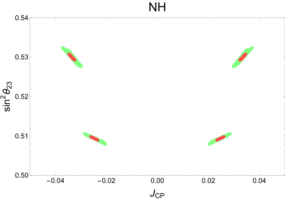
Figure 1: Predicted CP violation versus atmospheric angle for NH. Green (Red) regions correspond to 3 (1) σ\sigma values for the solar and reactor angles in Eqs. (63), (64). All predicted values for sin2⁡θ23\sin^{2}\theta_{23} lie inside its 1σ\sigma region, according to the global fit [47].

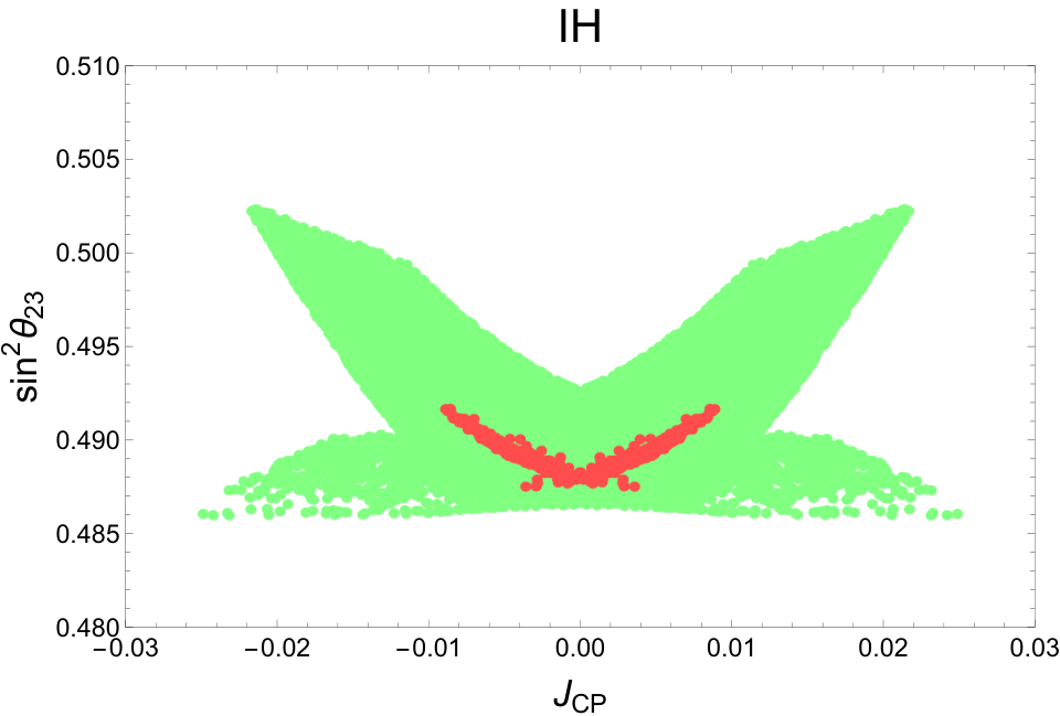
In figures 1 and 2, we give the allowed values for sin2⁡θ23\sin^{2}\theta_{23} together with the corresponding JCPJ_{\text{CP}} predictions in both mass orderings. For our analysis, we randomly generated parameter configurations for ω23\omega_{23}, ω13\omega_{13} and ψ\psi corresponding to 3(1)σ\sigma values for the solar and reactor angles in Eqs. (63),(64). One sees that for the Normal Hierarchy (NH) case the allowed region is severely restricted, with a fourfold degeneracy. In this case CP must necessarily be violated in oscillations, and the predicted atmospheric angle lies in the higher octant, inside its 1​σ1\sigma region.

Refer to caption
Figure 2: Predicted CP violation versus atmospheric angle for IH. Green (Red) regions correspond to 3 (1) σ\sigma values for the solar and reactor angles in Eqs. (63), (64). All predicted values for sin2⁡θ23\sin^{2}\theta_{23} in this case lie into its 2σ\sigma region [47].

In contrast, for the case of Inverted Hierarchy (IH) one sees that CP can be conserved in neutrino oscillations. Moreover, if violated, it is unlikely for CP to be maximally violated. The predicted atmospheric angle lies inside its 2​σ2\sigma region, preferably in the first octant.

6 Neutrinoless double beta decay

In this section we determine the effective Majorana neutrino mass parameter characterizing the neutrinoless double beta (0​ν​β​β0\nu\beta\beta) decay amplitude. It is given by:

|mβ​β|=|∑i=13miν​Ue​i2|=14|m1(2cosθ0cosω12cosω13+2e−i​ω23sinθ0[sinω12+isinω13cosω12])2+m2(−2cosθ0sinω12cosω13+2e−i​ω23sinθ0[cosω12−isinω12sinω13])2−m3(2e−i​ω23sinθ0cosω13+2icosθ0sinω13)2|,\begin{split}\left|m_{\beta\beta}\right|=&\left|\sum_{i=1}^{3}m^{\nu}_{i}U_{ei}^{2}\right|\\ =&\frac{1}{4}\bigg|m_{1}\left(2\cos\theta_{0}\cos\omega_{12}\cos\omega_{13}+\sqrt{2}e^{-i\omega_{23}}\sin\theta_{0}\left[\sin\omega_{12}+i\sin\omega_{13}\cos\omega_{12}\right]\right){}^{2}\\ &+m_{2}\left(-2\cos\theta_{0}\sin\omega_{12}\cos\omega_{13}+\sqrt{2}e^{-i\omega_{23}}\sin\theta_{0}\left[\cos\omega_{12}-i\sin\omega_{12}\sin\omega_{13}\right]\right){}^{2}\\ &-m_{3}\left(\sqrt{2}e^{-i\omega_{23}}\sin\theta_{0}\cos\omega_{13}+2i\cos\theta_{0}\sin\omega_{13}\right){}^{2}\bigg|,\end{split} (72)

where Ue​i2U_{ei}^{2} and mνim_{\nu_{i}} are the lepton mixing matrix elements and the light active neutrino masses, respectively. The light active neutrino masses can be written in terms of the parameters of the model as

m1=λ2​vξ2+r2{2tanω13sin2(ψ−ω23)+(1−4tan2ω13)cos(2ψ+ω23)−cos3ω232tanω13[2sin(ψ+2ω23)+2tanω13cos(ψ−ω23)]−(3​cos⁡2​ω13−1)​cos⁡(2​ψ+ω23)+(cos⁡2​ω13−3)​cos⁡3​ω232​2​sin⁡2​ω13​sin⁡(ψ+2​ω23)×1+16sin2ω13[sin(2ψ+ω23)+sin(3ω23)]2[(3cos2ω13−1)cos(2ψ+ω23)+(cos2ω13−3)cos3ω23]2},m2=λ2​vξ2+r2{2tanω13sin2(ψ−ω23)+(1−4tan2ω13)cos(2ψ+ω23)−cos3ω232tanω13[2sin(ψ+2ω23)+2tanω13cos(ψ−ω23)]+(3​cos⁡2​ω13−1)​cos⁡(2​ψ+ω23)+(cos⁡2​ω13−3)​cos⁡3​ω232​2​sin⁡2​ω13​sin⁡(ψ+2​ω23)×1+16sin2ω13[sin(2ψ+ω23)+sin(3ω23)]2[(3cos2ω13−1)cos(2ψ+ω23)+(cos2ω13−3)cos3ω23]2},m3=λ2​vξ2+r2​{tan2ω13[cos(ψ+2ω23)+cos3ψ]csc2(ψ+2ω23)−2cotω13sin(ψ−ω23)1+2tanω13cos(ψ−ω23)csc(ψ+2ω23)},\begin{split}m_{1}=&\frac{\lambda_{2}v_{\xi}}{\sqrt{2+r^{2}}}\bigg\{\frac{\sqrt{2}\tan\omega_{13}\sin 2\left(\psi-\omega_{23}\right)+\left(1-4\tan^{2}\omega_{13}\right)\cos\left(2\psi+\omega_{23}\right)-\cos 3\omega_{23}}{2\tan\omega_{13}\left[\sqrt{2}\sin\left(\psi+2\omega_{23}\right)+2\tan\omega_{13}\cos\left(\psi-\omega_{23}\right)\right]}\\ &\qquad-\frac{\left(3\cos 2\omega_{13}-1\right)\cos\left(2\psi+\omega_{23}\right)+\left(\cos 2\omega_{13}-3\right)\cos 3\omega_{23}}{2\sqrt{2}\sin 2\omega_{13}\sin\left(\psi+2\omega_{23}\right)}\\ &\qquad\times\sqrt{1+\frac{16\sin^{2}\omega_{13}\left[\sin\left(2\psi+\omega_{23}\right)+\sin\left(3\omega_{23}\right)\right]{}^{2}}{\left[\left(3\cos 2\omega_{13}-1\right)\cos\left(2\psi+\omega_{23}\right)+\left(\cos 2\omega_{13}-3\right)\cos 3\omega_{23}\right]{}^{2}}}\bigg\}\,,\\ m_{2}=&\frac{\lambda_{2}v_{\xi}}{\sqrt{2+r^{2}}}\bigg\{\frac{\sqrt{2}\tan\omega_{13}\sin 2\left(\psi-\omega_{23}\right)+\left(1-4\tan^{2}\omega_{13}\right)\cos\left(2\psi+\omega_{23}\right)-\cos 3\omega_{23}}{2\tan\omega_{13}\left[\sqrt{2}\sin\left(\psi+2\omega_{23}\right)+2\tan\omega_{13}\cos\left(\psi-\omega_{23}\right)\right]}\\ &\qquad+\frac{\left(3\cos 2\omega_{13}-1\right)\cos\left(2\psi+\omega_{23}\right)+\left(\cos 2\omega_{13}-3\right)\cos 3\omega_{23}}{2\sqrt{2}\sin 2\omega_{13}\sin\left(\psi+2\omega_{23}\right)}\\ &\qquad\times\sqrt{1+\frac{16\sin^{2}\omega_{13}\left[\sin\left(2\psi+\omega_{23}\right)+\sin\left(3\omega_{23}\right)\right]{}^{2}}{\left[\left(3\cos 2\omega_{13}-1\right)\cos\left(2\psi+\omega_{23}\right)+\left(\cos 2\omega_{13}-3\right)\cos 3\omega_{23}\right]{}^{2}}}\bigg\}\,,\\ m_{3}=&\frac{\lambda_{2}v_{\xi}}{\sqrt{2+r^{2}}}\bigg\{\frac{\tan^{2}\omega_{13}\left[\cos\left(\psi+2\omega_{23}\right)+\cos 3\psi\right]\csc^{2}\left(\psi+2\omega_{23}\right)-\sqrt{2}\cot\omega_{13}\sin\left(\psi-\omega_{23}\right)}{1+\sqrt{2}\tan\omega_{13}\cos\left(\psi-\omega_{23}\right)\csc\left(\psi+2\omega_{23}\right)}\bigg\}\,,\end{split} (73)

with

QνT​diag​(m1,m2,m3)​Qν=diag⁡(m1ν,m2ν,m3ν).Q_{\nu}^{T}\mathrm{diag}(m_{1},m_{2},m_{3})Q_{\nu}=\mathrm{diag}(m^{\nu}_{1},m^{\nu}_{2},m^{\nu}_{3}).

We show in Figure 3 the effective Majorana neutrino mass parameter |mβ​β||m_{\beta\beta}| versus the lightest active neutrino mass for the cases of normal and inverted neutrino mass hierarchies. In order to determine the predicted ranges for |mβ​β||m_{\beta\beta}| in our model, we have randomly generated the angles ω23\omega_{23}, ω13\omega_{13} and ψ\psi, as well as the light active neutrino mass scale mν=λ2​vξ2+r2m_{\nu}=\frac{\lambda_{2}v_{\xi}}{\sqrt{2+r^{2}}} in a range of values where the neutrino mass squared splittings and the leptonic mixing parameters are consistent with the observed neutrino oscillation data. Our predicted range of values for the effective Majorana neutrino mass parameter has a lower bound, even in the case of normal hierarchy, indicating that a complete destructive interference among the three light neutrinos is prevented by our symmetry and the current oscillation data.

The corresponding 0​ν​β​β\rm 0\nu\beta\beta decay rates are within the reach of the next-generation bolometric CUORE experiment [48] or, more realistically, of the next-to-next-generation ton-scale 0​ν​β​β0\nu\beta\beta-decay experiments. It is worth mentioning that the Majorana neutrino mass parameter has an upper bound on |mβ​β|≤(61−165)|m_{\beta\beta}|\leq(61-165) meV at 90% C.L, as indicated by the KamLAND-Zen experiment from the limit on the Xe136{}^{136}\mathrm{Xe} 0​ν​β​β0\nu\beta\beta decay half-life T1/20​ν​β​β​(Xe136)≥1.07×1026T^{0\nu\beta\beta}_{1/2}({}^{136}\mathrm{Xe})\geq 1.07\times 10^{26} yr [49]. This bound will be improved within a not too far future. The GERDA “phase-II”experiment [50, 51] is expected to reach T1/20​ν​β​β(76Ge)≥2×1026T^{0\nu\beta\beta}_{1/2}(^{76}{\rm Ge})\geq 2\times 10^{26} yr, corresponding to |mβ​β|≤100|m_{\beta\beta}|\leq 100 meV. A bolometric CUORE experiment, using Te130{}^{130}\mathrm{Te} [48], is currently under construction and its estimated sensitivity is close to about T1/20​ν​β​β(130Te)∼1026T_{1/2}^{0\nu\beta\beta}(^{130}\mathrm{Te})\sim 10^{26} yr, implying |mβ​β|≤50|m_{\beta\beta}|\leq 50 meV. Furthermore, there are plans for ton-scale next-to-next generation 0​ν​β​β0\nu\beta\beta experiments with 136Xe [52, 53] and 76Ge [50, 54], asserting sensitivities over T1/20​ν​β​β∼1027T_{1/2}^{0\nu\beta\beta}\sim 10^{27} yr, corresponding to |mβ​β|∼12−30|m_{\beta\beta}|\sim 12-30 meV.

Figure 3: Effective Majorana neutrino mass parameter |mβ​β||m_{\beta\beta}| as a function of the lightest active neutrino mass mlightestm_{\text{lightest}}. The light shaded regions indicate the 3σ\sigma ranges calculated from the oscillation parameter uncertainties [47], and the dark shaded areas correspond to the allowed values predicted by the model. The horizontal blue band indicates 90% C.L. upper limits on |mβ​β||m_{\beta\beta}| with 136Xe from the KamLAND-Zen experiment [49].

7 Discussions and Conclusions

We have proposed a realistic extension of the standard model within the Pati-Salam framework. The theory incorporates a flavor symmetry based on the Δ⁡(27)\Delta\left(27\right) group and realizes a realistic Froggatt-Nielsen picture of quark mixing. Concerning the lepton sector, neutrino masses arise from an inverse seesaw mechanism and the allowed ranges for the atmospheric mixing angle θ23\theta_{23} and CP violating phase δC​P\delta_{CP} are rather restricted once one takes into account the precise measurements of the remaining oscillation parameters. This makes the model rather predictive. Our main neutrino oscillation results are summarized in Figs. 1 and 2. We find that, for normal neutrino mass ordering, the atmospheric angle must lie in the higher octant and that CP must be violated in oscillations. In contrast, for inverse hierarchy, the lower octant is favored and the range of allowed Jarlskog invariant extends from zero up to a non-maximal value. Our results concerning 0​ν​β​β\rm 0\nu\beta\beta decay are summarized in Fig.3. They indicate the existence of a lower bound for the 0​ν​β​β\rm 0\nu\beta\beta decay rate, a feature also encountered in other flavor models [55, 56, 57, 58, 59]. As mentioned, neutrino masses arise from a low-scale seesaw mechanism, whose messengers may be produced at the LHC either through a charged or neutral gauge portal [16, 14, 60]. Admittedly, the model is rather complex, especially in its scalar sector. However, it serves as a “proof-of-concept” attempt, namely, to our knowledge this is the first time that a fully realistic and to some extent predictive flavor realization of a Pati-Salam scenario is given.

Acknowledgments

This research is supported by the Spanish grants FPA2014-58183-P, Multidark CSD2009-00064, SEV-2014-0398 (MINECO) and PROMETEOII/2014/084 (Generalitat Valenciana); Chilean grants Fondecyt No. 1170803, No. 1150792 and CONICYT PIA/Basal FB0821 and ACT1406; and Mexican grant CONACYT No. 274397. A.E.C.H is very grateful to Professor Hoang Ngoc Long and the other members of its group for the warm hospitality of the Institute of Physics, Vietnam Academy of Science and Technology, where this work was completed.

Appendix

Appendix A Product rules of the Δ⁡(27)\Delta(27) discrete group

The Δ⁡(27)\Delta(27) discrete group is a subgroup of S​U​(3)SU(3), has 27 elements divided into 11 conjugacy classes, so that it has 11 irreducible representations. These irreducible representations are: two triplets, i.e., 𝟑[0]​[1]\mathbf{3}_{[0][1]} (which we denote by 𝟑\mathbf{3}) and its conjugate 𝟑[0]​[2]\mathbf{3}_{[0][2]} (which we denote by 𝟑¯\overline{\mathbf{3}}) and 9 singlets, i.e., 𝟏k,l\mathbf{1}_{k,l} (k,l=0,1,2k,l=0,1,2), where kk and ll correspond to the Z3Z_{3} and Z3′Z_{3}^{\prime} charges, respectively [4]. The Δ⁡(27)\Delta(27) discrete group is a simple group of the type Δ⁡(3​n2)\Delta(3n^{2}) with n=3n=3 and is isomorphic to the semi-direct product group (Z3′×Z3′′)⋊Z3(Z_{3}^{\prime}\times Z_{3}^{\prime\prime})\rtimes Z_{3} [4]. Indeed, the simplest group of the type Δ⁡(3​n2)\Delta(3n^{2}) is Δ⁡(3)≡Z3\Delta(3)\equiv Z_{3}. The next group is Δ⁡(12)\Delta(12), which is isomorphic to A4A_{4}. Thus, the Δ⁡(27)\Delta(27) discrete group is the next simplest nontrivial group of the type Δ⁡(3​n2)\Delta(3n^{2}). It is worth mentioning that one can write any element of the Δ⁡(27)\Delta(27) discrete group as bk​am​a′nb^{k}a^{m}{a^{\prime}}^{n}, where bb, aa and a′a^{\prime} correspond to the generators of the Z3Z_{3}, Z3′Z_{3}^{\prime} and Z3′′Z_{3}^{\prime\prime} cyclic groups, respectively. These generators fulfill the relations:

a3=a′3=b3=1,a​a′=a′​a,\displaystyle a^{3}=a^{\prime 3}=b^{3}=1,\hskip 14.22636ptaa^{\prime}=a^{\prime}a,
b​a​b−1=a−1​a′−1,b​a′​b−1=a,\displaystyle bab^{-1}=a^{-1}a^{\prime-1},\,\,ba^{\prime}b^{-1}=a, (74)

The characters of the Δ⁡(27)\Delta(27) discrete group are shown in Table 5. Here nn is the number of elements, hh is the order of each element, and ω=e2​π​i3=−12+i​32\omega=e^{\frac{2\pi i}{3}}=-\frac{1}{2}+i\frac{\sqrt{3}}{2} is the cube root of unity, which satisfies the relations 1+ω+ω2=01+\omega+\omega^{2}=0 and ω3=1\omega^{3}=1. The conjugacy classes of Δ⁡(27)\Delta(27) are given by:

C1:{e},h=1,C1(1):{a,a′2},h=3,C1(2):{a2,a′},h=3,C3(0,1):{a′2​a′2},h=3,C3(0,2):{a′2,a2,a​a′},h=3,C3(1,p):{b​ap,b​ap−1​a′p−2​a′2},h=3,C3(2,p):{b​ap,b​ap−1​a′p−2​a′2},h=3.\begin{array}[]{ccc}C_{1}:&\{e\},&h=1,\\ C_{1}^{(1)}:&\{a,a^{\prime 2}\},&h=3,\\ C_{1}^{(2)}:&\{a^{2},a^{\prime}\},&h=3,\\ C_{3}^{(0,1)}:&\{a^{\prime 2}a^{\prime 2}\},&h=3,\\ C_{3}^{(0,2)}:&\{a^{\prime 2},a^{2},aa^{\prime}\},&h=3,\\ C_{3}^{(1,p)}:&\{ba^{p},ba^{p-1}a^{\prime p-2}a^{\prime 2}\},&h=3,\\ C_{3}^{(2,p)}:&\{ba^{p},ba^{p-1}a^{\prime p-2}a^{\prime 2}\},&h=3.\\ &&\end{array}
h χ1(r,s)\chi_{1_{(r,s)}} χ3[0,1]\chi_{3_{[0,1]}} χ3[0,2]\chi_{3_{[0,2]}}
1​C11C_{1} 1 1 3 3
1​C1(1)1C_{1}^{(1)} 1 1 3​ω23\omega^{2} 3​ω3\omega
1​C1(2)1C_{1}^{(2)} 1 1 3​ω3\omega 3​ω23\omega^{2}
3​C1(0,1)3C_{1}^{(0,1)} 33 ωs\omega^{s} 00 00
3​C1(0,2)3C_{1}^{(0,2)} 33 ω2​s\omega^{2s} 00 00
C3(1,p)C_{3}^{(1,p)} 33 ωr+s​p\omega^{r+sp} 0 0
C3(2,p)C_{3}^{(2,p)} 33 ω2​r+s​p\omega^{2r+sp} 0 0
Table 5: Characters of Δ⁡(27)\Delta(27)

The tensor products between Δ⁡(27)\Delta(27) triplets are described by the following relations [4]:

(x1,−1x0,1x−1,0)𝟑⊗(y1,−1y0,1y−1,0)𝟑\displaystyle\vskip-28.45274pt\begin{pmatrix}x_{1,-1}\\ x_{0,1}\\ x_{-1,0}\\ \end{pmatrix}_{\mathbf{3}}\otimes\begin{pmatrix}y_{1,-1}\\ y_{0,1}\\ y_{-1,0}\\ \end{pmatrix}_{\mathbf{3}} =\displaystyle= (x1,−1​y1,−1x0,1​y0,1x−1,0​y−1,0)𝟑¯S1⊕12​(x0,1​y−1,0+x−1,0​y0,1x−1,0​y1,−1+x1,−1​y−1,0x1,−1​y0,1+x0,1​y1,−1)𝟑¯S2\displaystyle\begin{pmatrix}x_{1,-1}y_{1,-1}\\ x_{0,1}y_{0,1}\\ x_{-1,0}y_{-1,0}\\ \end{pmatrix}_{\mathbf{\bar{3}}_{S_{1}}}\oplus\frac{1}{2}\begin{pmatrix}x_{0,1}y_{-1,0}+x_{-1,0}y_{0,1}\\ x_{-1,0}y_{1,-1}+x_{1,-1}y_{-1,0}\\ x_{1,-1}y_{0,1}+x_{0,1}y_{1,-1}\\ \end{pmatrix}_{\mathbf{\bar{3}}_{S_{2}}} (75)
⊕12​(x0,1​y−1,0−x−1,0​y0,1x−1,0​y1,−1−x1,−1​y−1,0x1,−1​y0,1−x0,1​y1,−1)𝟑¯A,\displaystyle\oplus\frac{1}{2}\begin{pmatrix}x_{0,1}y_{-1,0}-x_{-1,0}y_{0,1}\\ x_{-1,0}y_{1,-1}-x_{1,-1}y_{-1,0}\\ x_{1,-1}y_{0,1}-x_{0,1}y_{1,-1}\\ \end{pmatrix}_{\mathbf{\bar{3}}_{A}},
(x2,−2x0,2x−2,0)𝟑¯⊗(y2,−2y0,2y−2,0)𝟑¯\displaystyle\begin{pmatrix}x_{2,-2}\\ x_{0,2}\\ x_{-2,0}\\ \end{pmatrix}_{\mathbf{\bar{3}}}\otimes\begin{pmatrix}y_{2,-2}\\ y_{0,2}\\ y_{-2,0}\\ \end{pmatrix}_{\mathbf{\bar{3}}} =\displaystyle= (x2,−2​y2,−2x0,2​y0,2x−2,0​y−2,0)𝟑S1⊕12​(x0,2​y−2,0+x−2,0​y0,2x−2,0​y2,−2+x2,−2​y−2,0x2,−2​y0,2+x0,2​y2,−2)𝟑S2\displaystyle\begin{pmatrix}x_{2,-2}y_{2,-2}\\ x_{0,2}y_{0,2}\\ x_{-2,0}y_{-2,0}\\ \end{pmatrix}_{\mathbf{3}_{S_{1}}}\oplus\frac{1}{2}\begin{pmatrix}x_{0,2}y_{-2,0}+x_{-2,0}y_{0,2}\\ x_{-2,0}y_{2,-2}+x_{2,-2}y_{-2,0}\\ x_{2,-2}y_{0,2}+x_{0,2}y_{2,-2}\\ \end{pmatrix}_{\mathbf{3}_{S_{2}}} (76)
⊕12​(x0,2​y−2,0−x−2,0​y0,2x−2,0​y2,−2−x2,−2​y−2,0x2,−2​y0,2−x0,2​y2,−2)𝟑A,\displaystyle\oplus\frac{1}{2}\begin{pmatrix}x_{0,2}y_{-2,0}-x_{-2,0}y_{0,2}\\ x_{-2,0}y_{2,-2}-x_{2,-2}y_{-2,0}\\ x_{2,-2}y_{0,2}-x_{0,2}y_{2,-2}\\ \end{pmatrix}_{\mathbf{3}_{A}},
(x1,−1x0,1x−1,0)𝟑⊗(y−1,1y0,−1y1,0)𝟑¯\displaystyle\begin{pmatrix}x_{1,-1}\\ x_{0,1}\\ x_{-1,0}\\ \end{pmatrix}_{\mathbf{3}}\otimes\begin{pmatrix}y_{-1,1}\\ y_{0,-1}\\ y_{1,0}\\ \end{pmatrix}_{\mathbf{\bar{3}}} =\displaystyle= ∑r(x1,−1​y−1,1+ω2​r​x0,1​y0,−1+ωr​x−1,0​y1,0)𝟏(r,0)\displaystyle\sum_{r}(x_{1,-1}y_{-1,1}+\omega^{2r}x_{0,1}y_{0,-1}+\omega^{r}x_{-1,0}y_{1,0})_{\mathbf{1}_{(r,0)}}
⊕\displaystyle\oplus ∑r(x1,−1​y0,−1+ω2​r​x0,1​y1,0+ωr​x−1,0​y−1,1)𝟏(r,1)\displaystyle\sum_{r}(x_{1,-1}y_{0,-1}+\omega^{2r}x_{0,1}y_{1,0}+\omega^{r}x_{-1,0}y_{-1,1})_{\mathbf{1}_{(r,1)}}
⊕\displaystyle\oplus ∑r(x1,−1​y1,0+ω2​r​x0,1​y−1,1+ωr​x−1,0​y0,−1)𝟏(r,2),\displaystyle\sum_{r}(x_{1,-1}y_{1,0}+\omega^{2r}x_{0,1}y_{-1,1}+\omega^{r}x_{-1,0}y_{0,-1})_{\mathbf{1}_{(r,2)}},

where we introduced the shorthand notation 𝟑[0]​[1]≡𝟑\mathbf{3}_{[0][1]}\equiv\mathbf{3} and 𝟑[0]​[2]≡𝟑¯\mathbf{3}_{[0][2]}\equiv\mathbf{\bar{3}} used in Eq.(8). In the above formulas 𝟑A\mathbf{3}_{A} and 𝟑S1,2\mathbf{3}_{S_{1,2}} are an antisymmetric and two variants of symmetric triplets. The multiplication rules between Δ⁡(27)\Delta(27) singlets and Δ⁡(27)\Delta(27) triplets are given by [4]:

(x(1,−1)x(0,1)x(−1,0))𝟑[0]​[1]⊗(z)1k,l=(x(1,−1)​zωr​x(0,1)​zω2​r​x(−1,0)​z)𝟑[l]​[1+l],\displaystyle\begin{pmatrix}x_{(1,-1)}\\ x_{(0,1)}\\ x_{(-1,0)}\end{pmatrix}_{\mathbf{3}_{[0][1]}}\otimes(z)_{1_{k,l}}=\begin{pmatrix}x_{(1,-1)}z\\ \omega^{r}x_{(0,1)}z\\ \omega^{2r}x_{(-1,0)}z\end{pmatrix}_{\mathbf{3}_{[l][1+l]}}, (78)
(x(2,−2)x(0,2)x(−2,0))𝟑[0]​[2]⊗(z)1k,l=(x(2,−2)​zωr​x(0,2)​zω2​r​x(−2,0))𝟑[l]​[2+l].\displaystyle\begin{pmatrix}x_{(2,-2)}\\ x_{(0,2)}\\ x_{(-2,0)}\end{pmatrix}_{\mathbf{3}_{[0][2]}}\otimes(z)_{1_{k,l}}=\begin{pmatrix}x_{(2,-2)}z\\ \omega^{r}x_{(0,2)}z\\ \omega^{2r}x_{(-2,0)}\end{pmatrix}_{\mathbf{3}_{[l][2+l]}}. (79)

The tensor products of Δ⁡(27)\Delta(27) singlets 𝟏k,ℓ\mathbf{1}_{k,\ell} and 𝟏k′,ℓ′\mathbf{1}_{k^{\prime},\ell^{\prime}} take the form [4]:

𝟏k,ℓ⊗𝟏k′,ℓ′=𝟏k+k′​mod​ 3,ℓ+ℓ′​mod​ 3.\mathbf{1}_{k,\ell}\otimes\mathbf{1}_{k^{\prime},\ell^{\prime}}=\mathbf{1}_{k+k^{\prime}\mathrm{\,mod\,}3,\ell+\ell^{\prime}\mathrm{\,mod\,}3}. (80)

From the equation given above, we obtain explicitly the singlet multiplication rules of the Δ⁡(27)\Delta(27) group, which are given in Table 6.

Singlets 𝟏01\mathbf{1}_{01} 𝟏02\mathbf{1}_{02} 𝟏10\mathbf{1}_{10} 𝟏11\mathbf{1}_{11} 𝟏12\mathbf{1}_{12} 𝟏20\mathbf{1}_{20} 𝟏21\mathbf{1}_{21} 𝟏22\mathbf{1}_{22}
𝟏01\mathbf{1}_{01} 𝟏02\mathbf{1}_{02} 𝟏00\mathbf{1}_{00} 𝟏11\mathbf{1}_{11} 𝟏12\mathbf{1}_{12} 𝟏10\mathbf{1}_{10} 𝟏21\mathbf{1}_{21} 𝟏22\mathbf{1}_{22} 𝟏20\mathbf{1}_{20}
𝟏02\mathbf{1}_{02} 𝟏00\mathbf{1}_{00} 𝟏01\mathbf{1}_{01} 𝟏12\mathbf{1}_{12} 𝟏10\mathbf{1}_{10} 𝟏11\mathbf{1}_{11} 𝟏22\mathbf{1}_{22} 𝟏20\mathbf{1}_{20} 𝟏21\mathbf{1}_{21}
𝟏10\mathbf{1}_{10} 𝟏11\mathbf{1}_{11} 𝟏12\mathbf{1}_{12} 𝟏20\mathbf{1}_{20} 𝟏21\mathbf{1}_{21} 𝟏22\mathbf{1}_{22} 𝟏00\mathbf{1}_{00} 𝟏01\mathbf{1}_{01} 𝟏02\mathbf{1}_{02}
𝟏11\mathbf{1}_{11} 𝟏12\mathbf{1}_{12} 𝟏10\mathbf{1}_{10} 𝟏21\mathbf{1}_{21} 𝟏22\mathbf{1}_{22} 𝟏20\mathbf{1}_{20} 𝟏01\mathbf{1}_{01} 𝟏02\mathbf{1}_{02} 𝟏00\mathbf{1}_{00}
𝟏12\mathbf{1}_{12} 𝟏10\mathbf{1}_{10} 𝟏11\mathbf{1}_{11} 𝟏22\mathbf{1}_{22} 𝟏20\mathbf{1}_{20} 𝟏21\mathbf{1}_{21} 𝟏02\mathbf{1}_{02} 𝟏00\mathbf{1}_{00} 𝟏01\mathbf{1}_{01}
𝟏20\mathbf{1}_{20} 𝟏21\mathbf{1}_{21} 𝟏22\mathbf{1}_{22} 𝟏00\mathbf{1}_{00} 𝟏01\mathbf{1}_{01} 𝟏02\mathbf{1}_{02} 𝟏10\mathbf{1}_{10} 𝟏11\mathbf{1}_{11} 𝟏12\mathbf{1}_{12}
𝟏21\mathbf{1}_{21} 𝟏22\mathbf{1}_{22} 𝟏20\mathbf{1}_{20} 𝟏01\mathbf{1}_{01} 𝟏02\mathbf{1}_{02} 𝟏00\mathbf{1}_{00} 𝟏11\mathbf{1}_{11} 𝟏12\mathbf{1}_{12} 𝟏10\mathbf{1}_{10}
𝟏22\mathbf{1}_{22} 𝟏20\mathbf{1}_{20} 𝟏21\mathbf{1}_{21} 𝟏02\mathbf{1}_{02} 𝟏00\mathbf{1}_{00} 𝟏01\mathbf{1}_{01} 𝟏12\mathbf{1}_{12} 𝟏10\mathbf{1}_{10} 𝟏11\mathbf{1}_{11}
Table 6: The singlet multiplications of the group Δ⁡(27)\Delta(27).

Appendix B Scalar potential for one Δ⁡(27)\Delta(27) scalar triplet

The scalar potential for a Δ⁡(27)\Delta(27) scalar triplet, i.e., ξ\xi is given by:

V\displaystyle V =\displaystyle= −μξ2​(ξ​ξ∗)𝟏𝟎,𝟎+κ1​(ξ​ξ∗)𝟏𝟎,𝟎​(ξ​ξ∗)𝟏𝟎,𝟎+κ2​(ξ​ξ∗)𝟏𝟏,𝟎​(ξ​ξ∗)𝟏𝟐,𝟎+κ3​(ξ​ξ∗)𝟏𝟎,𝟏​(ξ​ξ∗)𝟏𝟎,𝟐\displaystyle-\mu_{\xi}^{2}\left(\xi\xi^{\ast}\right)_{\mathbf{\mathbf{1}_{0\mathbf{,0}}}}+\kappa_{1}\left(\xi\xi^{\ast}\right)_{\mathbf{\mathbf{1}_{0\mathbf{,0}}}}\left(\xi\xi^{\ast}\right)_{\mathbf{\mathbf{1}_{0\mathbf{,0}}}}+\kappa_{2}\left(\xi\xi^{\ast}\right)_{\mathbf{\mathbf{1}_{1\mathbf{,0}}}}\left(\xi\xi^{\ast}\right)_{\mathbf{\mathbf{1}_{2\mathbf{,0}}}}+\kappa_{3}\left(\xi\xi^{\ast}\right)_{\mathbf{\mathbf{1}_{0,1}}}\left(\xi\xi^{\ast}\right)_{\mathbf{\mathbf{1}_{0,2}}} (81)
+κ4[(ξξ∗)𝟏𝟏,𝟏(ξξ∗)𝟏𝟐,𝟐+h.c.]+κ5(ξξ)𝟑¯𝐒𝟏(ξ∗ξ∗)𝟑S1+κ6(ξξ)𝟑¯𝐒𝟐(ξ∗ξ∗)𝟑S2\displaystyle+\kappa_{4}\left[\left(\xi\xi^{\ast}\right)_{\mathbf{\mathbf{1}_{1,1}}}\left(\xi\xi^{\ast}\right)_{\mathbf{\mathbf{1}_{2,2}}}+\text{h.c.}\right]+\kappa_{5}\left(\xi\xi\right)_{\overline{\mathbf{3}}\mathbf{{}_{S_{1}}}}\left(\xi^{\ast}\xi^{\ast}\right)_{\mathbf{3}_{S_{1}}}+\kappa_{6}\left(\xi\xi\right)_{\overline{\mathbf{3}}\mathbf{{}_{S_{2}}}}\left(\xi^{\ast}\xi^{\ast}\right)_{\mathbf{3}_{S_{2}}}
+κ7[(ξξ)𝟑¯𝐒𝟏(ξ∗ξ∗)𝟑S2+h.c.]\displaystyle+\kappa_{7}\left[\left(\xi\xi\right)_{\overline{\mathbf{3}}\mathbf{{}_{S_{1}}}}\left(\xi^{\ast}\xi^{\ast}\right)_{\mathbf{3}_{S_{2}}}+\text{h.c.}\right]

Assuming the VEV configuration for the Δ⁡(27)\Delta(27) scalar triplet ξ\xi:

⟨ξ⟩=vξ2+r2​(r,e−i​ψ,ei​ψ),\left\langle\xi\right\rangle=\frac{v_{\xi}}{\sqrt{2+r^{2}}}\left(r,e^{-i\psi},e^{i\psi}\right), (82)

We find that the scalar potential minimization equations are:

∂V∂ξ1\displaystyle\frac{\partial V}{\partial\xi\text{${}_{{}_{1}}$}} =\displaystyle= 2​vξ3​{(2​κ3+κ4+2​κ7)​cos⁡ψ+r⁡[2​κ3+κ4+2​κ7+2​(κ1+κ2+κ5)​r2]}(r2+2)3/2\displaystyle\frac{2v_{\xi}^{3}\left\{\left(2\kappa_{3}+\kappa_{4}+2\kappa_{7}\right)\cos\psi+r\left[2\kappa_{3}+\kappa_{4}+2\kappa_{7}+2\left(\kappa_{1}+\kappa_{2}+\kappa_{5}\right)r^{2}\right]\right\}}{\left(r^{2}+2\right)^{3/2}}
+2​vξ​[2​(2​κ1−κ2+κ3−κ4+κ6)​r​vξ2​cos⁡2​ψ−μξ2​r​(r2+2)](r2+2)3/2\displaystyle+\frac{2v_{\xi}\left[2\left(2\kappa_{1}-\kappa_{2}+\kappa_{3}-\kappa_{4}+\kappa_{6}\right)rv_{\xi}^{2}\cos 2\psi-\mu_{\xi}^{2}r\left(r^{2}+2\right)\right]}{\left(r^{2}+2\right)^{3/2}}
=\displaystyle= 0\displaystyle 0\,
∂V∂ξ2\displaystyle\frac{\partial V}{\partial\xi\text{${}_{2}$}} =\displaystyle= e−3​i​ψ​vξ3​[4​(κ1+κ2+κ5)+2​(2​κ1−κ2+κ3−κ4+κ6)​r2​e2​i​ψ](r2+2)3/2\displaystyle\frac{e^{-3i\psi}v_{\xi}^{3}\left[4\left(\kappa_{1}+\kappa_{2}+\kappa_{5}\right)+2\left(2\kappa_{1}-\kappa_{2}+\kappa_{3}-\kappa_{4}+\kappa_{6}\right)r^{2}e^{2i\psi}\right]}{\left(r^{2}+2\right)^{3/2}}
+ei​ψ​vξ3​[4​κ1−2​κ2+2​κ6+2​κ7​r2+2​κ3​(r2+1)+κ4​(r2−2)](r2+2)3/2\displaystyle+\frac{e^{i\psi}v_{\xi}^{3}\left[4\kappa_{1}-2\kappa_{2}+2\kappa_{6}+2\kappa_{7}r^{2}+2\kappa_{3}\left(r^{2}+1\right)+\kappa_{4}\left(r^{2}-2\right)\right]}{\left(r^{2}+2\right)^{3/2}}
+e−3​i​ψ​{vξ3​[2​(2​κ3+κ4+2​κ7)​r​e3​i​ψ+(2​κ3+κ4+2​κ7)​r​e5​i​ψ]−2​μξ2​(r2+2)​e2​i​ψ​vξ}(r2+2)3/2\displaystyle+\frac{e^{-3i\psi}\left\{v_{\xi}^{3}\left[2\left(2\kappa_{3}+\kappa_{4}+2\kappa_{7}\right)re^{3i\psi}+\left(2\kappa_{3}+\kappa_{4}+2\kappa_{7}\right)re^{5i\psi}\right]-2\mu_{\xi}^{2}\left(r^{2}+2\right)e^{2i\psi}v_{\xi}\right\}}{\left(r^{2}+2\right)^{3/2}}
=\displaystyle= 0,\displaystyle 0,\hskip 14.22636pt\hskip 14.22636pt\hskip 14.22636pt\hskip 14.22636pt
∂V∂ξ3\displaystyle\frac{\partial V}{\partial\xi\text{${}_{3}$}} =\displaystyle= e−2​i​ψ​vξ3​[4​(κ1+κ2+κ5)​e5​i​ψ+2​(2​κ1−κ2+κ3−κ4+κ6)​r2​e3​i​ψ](r2+2)3/2\displaystyle\frac{e^{-2i\psi}v_{\xi}^{3}\left[4\left(\kappa_{1}+\kappa_{2}+\kappa_{5}\right)e^{5i\psi}+2\left(2\kappa_{1}-\kappa_{2}+\kappa_{3}-\kappa_{4}+\kappa_{6}\right)r^{2}e^{3i\psi}\right]}{\left(r^{2}+2\right)^{3/2}} (83)
+e−2​i​ψ​vξ3​[ei​ψ​(4​κ1−2​κ2+2​κ6+2​κ7​r2+2​κ3​(r2+1)+κ4​(r2−2))](r2+2)3/2\displaystyle+\frac{e^{-2i\psi}v_{\xi}^{3}\left[e^{i\psi}\left(4\kappa_{1}-2\kappa_{2}+2\kappa_{6}+2\kappa_{7}r^{2}+2\kappa_{3}\left(r^{2}+1\right)+\kappa_{4}\left(r^{2}-2\right)\right)\right]}{\left(r^{2}+2\right)^{3/2}}
+e−2​i​ψ​{vξ3​[2​(2​κ3+κ4+2​κ7)​r​e2​i​ψ+(2​κ3+κ4+2​κ7)​r]−2​μξ2​(r2+2)​e3​i​ψ​vξ}(r2+2)3/2\displaystyle+\frac{e^{-2i\psi}\left\{v_{\xi}^{3}\left[2\left(2\kappa_{3}+\kappa_{4}+2\kappa_{7}\right)re^{2i\psi}+\left(2\kappa_{3}+\kappa_{4}+2\kappa_{7}\right)r\right]-2\mu_{\xi}^{2}\left(r^{2}+2\right)e^{3i\psi}v_{\xi}\right\}}{\left(r^{2}+2\right)^{3/2}}
=\displaystyle= 0.\displaystyle 0.

Then, from the scalar potential minimization equations, we find the following relations:

μξ2\displaystyle\mu_{\xi}^{2} =\displaystyle= vξ2r⁡(r2+2){(2κ3+κ4+2κ7)cosψ+r[2κ3+κ4+2κ7+2(κ1+κ2+κ5)r2]\displaystyle\frac{v_{\xi}^{2}}{r\left(r^{2}+2\right)}\bigg\{\left(2\kappa_{3}+\kappa_{4}+2\kappa_{7}\right)\cos\psi+r\left[2\kappa_{3}+\kappa_{4}+2\kappa_{7}+2\left(\kappa_{1}+\kappa_{2}+\kappa_{5}\right)r^{2}\right] (84)
+2(2κ1−κ2+κ3−κ4+κ6)rcos2ψ},\displaystyle+2\left(2\kappa_{1}-\kappa_{2}+\kappa_{3}-\kappa_{4}+\kappa_{6}\right)r\cos 2\psi\bigg\},
2​[−6​κ2−4​κ5+2​κ6+2​κ7​r2+2​κ3​(r2+1)+κ4​(r2−2)]​sin⁡ψ​cos⁡ψ\displaystyle 2\left[-6\kappa_{2}-4\kappa_{5}+2\kappa_{6}+2\kappa_{7}r^{2}+2\kappa_{3}\left(r^{2}+1\right)+\kappa_{4}\left(r^{2}-2\right)\right]\sin\psi\cos\psi
+[2​(2​κ3+κ4+2​κ7)​r​cos⁡2​ψ+3​(2​κ3+κ4+2​κ7)​r]​sin⁡ψ=0,\displaystyle+\left[2\left(2\kappa_{3}+\kappa_{4}+2\kappa_{7}\right)r\cos 2\psi+3\left(2\kappa_{3}+\kappa_{4}+2\kappa_{7}\right)r\right]\sin\psi=0,
(2​κ3+κ4+2​κ7)​(r2−1)​cos⁡2​ψ\displaystyle\left(2\kappa_{3}+\kappa_{4}+2\kappa_{7}\right)\left(r^{2}-1\right)\cos 2\psi
−r⁡{2​(2​κ3+κ4+2​κ7)+[6​κ2−4​κ3+κ4+4​κ5−2​(κ6+κ7)]​r2}​cos⁡ψ\displaystyle-r\left\{2\left(2\kappa_{3}+\kappa_{4}+2\kappa_{7}\right)+\left[6\kappa_{2}-4\kappa_{3}+\kappa_{4}+4\kappa_{5}-2\left(\kappa_{6}+\kappa_{7}\right)\right]r^{2}\right\}\cos\psi
+(2​κ3+κ4+2​κ7)​(2​r2−1)+2​(3​κ2−κ3+κ4+2​κ5−κ6)​r​cos⁡3​ψ=0.\displaystyle+\left(2\kappa_{3}+\kappa_{4}+2\kappa_{7}\right)\left(2r^{2}-1\right)+2\left(3\kappa_{2}-\kappa_{3}+\kappa_{4}+2\kappa_{5}-\kappa_{6}\right)r\cos 3\psi=0.

Thus, the VEV pattern for the Δ⁡(27)\Delta(27) triplet, i.e., ξ\xi given by Eq. (82), is compatible with a global minimum of the scalar potential of Eq. (81) for a large region of parameter space.

Appendix C Scalar potential for three Δ⁡(27)\Delta(27) scalar triplets

The scalar potential for the three Δ⁡(27)\Delta(27) scalar triplets ρ\rho, τ\tau and η\eta is

V=Vρ+Vτ+Vη+Vρ,τ+Vτ,η+Vρ,η,V=V_{\rho}+V_{\tau}+V_{\eta}+V_{\rho,\tau}+V_{\tau,\eta}+V_{\rho,\eta}\,, (85)

where VρV_{\rho}, VτV_{\tau} and VηV_{\eta} are the scalar potentials for the Δ⁡(27)\Delta(27) scalar triplets ρ\rho, τ\tau and η\eta, respectively, whereas Vρ,τV_{\rho,\tau}, Vτ,ηV_{\tau,\eta} and Vρ,ηV_{\rho,\eta} describe interaction terms involving the pairs (ρ\rho, τ\tau), (τ\tau, η\eta) and (ρ\rho, η\eta). The different parts of the scalar potential for the three Δ⁡(27)\Delta(27) scalar triplets take the form:

Vρ\displaystyle V_{\rho} =\displaystyle= −μρ2​(ρ​ρ∗)𝟏𝟎,𝟎+κρ,1​(ρ​ρ∗)𝟏𝟎,𝟎​(ρ​ρ∗)𝟏𝟎,𝟎+κρ,2​(ρ​ρ∗)𝟏𝟏,𝟎​(ρ​ρ∗)𝟏𝟐,𝟎\displaystyle-\mu_{\rho}^{2}\left(\rho\rho^{\ast}\right)_{\mathbf{\mathbf{1}_{0\mathbf{,0}}}}+\kappa_{\rho,1}\left(\rho\rho^{\ast}\right)_{\mathbf{\mathbf{1}_{0\mathbf{,0}}}}\left(\rho\rho^{\ast}\right)_{\mathbf{\mathbf{1}_{0\mathbf{,0}}}}+\kappa_{\rho,2}\left(\rho\rho^{\ast}\right)_{\mathbf{\mathbf{1}_{1\mathbf{,0}}}}\left(\rho\rho^{\ast}\right)_{\mathbf{\mathbf{1}_{2\mathbf{,0}}}} (86)
+κρ,3(ρρ∗)𝟏𝟎,𝟏(ρρ∗)𝟏𝟎,𝟐+κρ,4[(ρρ∗)𝟏𝟏,𝟏(ρρ∗)𝟏𝟐,𝟐+h.c.]+κρ,5(ρρ)𝟑¯𝐒𝟏(ρ∗ρ∗)𝟑S1\displaystyle+\kappa_{\rho,3}\left(\rho\rho^{\ast}\right)_{\mathbf{\mathbf{1}_{0,1}}}\left(\rho\rho^{\ast}\right)_{\mathbf{\mathbf{1}_{0,2}}}+\kappa_{\rho,4}\left[\left(\rho\rho^{\ast}\right)_{\mathbf{\mathbf{1}_{1,1}}}\left(\rho\rho^{\ast}\right)_{\mathbf{\mathbf{1}_{2,2}}}+\text{h.c.}\right]+\kappa_{\rho,5}\left(\rho\rho\right)_{\overline{\mathbf{3}}\mathbf{{}_{S_{1}}}}\left(\rho^{\ast}\rho^{\ast}\right)_{\mathbf{3}_{S_{1}}}
+κρ,6(ρρ)𝟑¯𝐒𝟐(ρ∗ρ∗)𝟑S2+κρ,7[(ρρ)𝟑¯𝐒𝟏(ρ∗ρ∗)𝟑S2+h.c.],\displaystyle+\kappa_{\rho,6}\left(\rho\rho\right)_{\overline{\mathbf{3}}\mathbf{{}_{S_{2}}}}\left(\rho^{\ast}\rho^{\ast}\right)_{\mathbf{3}_{S_{2}}}+\kappa_{\rho,7}\left[\left(\rho\rho\right)_{\overline{\mathbf{3}}\mathbf{{}_{S_{1}}}}\left(\rho^{\ast}\rho^{\ast}\right)_{\mathbf{3}_{S_{2}}}+\text{h.c.}\right]\,,
Vτ\displaystyle V_{\tau} =\displaystyle= Vρ(ρ→τ,μρ→μτ,κρ,j→κτ,j),\displaystyle V_{\rho}\left(\rho\to\tau,\mu_{\rho}\to\mu_{\tau},\kappa_{\rho,j}\to\kappa_{\tau,j}\right)\,, (87)
Vη\displaystyle V_{\eta} =\displaystyle= Vρ(ρ→η,μρ→μη,κρ,j→κη,j),\displaystyle V_{\rho}\left(\rho\rightarrow\eta,\mu_{\rho}\to\mu_{\eta},\kappa_{\rho,j}\to\kappa_{\eta,j}\right)\,, (88)
Vρ,τ\displaystyle V_{\rho,\tau} =\displaystyle= γρ​τ,1​(ρ​ρ∗)𝟏𝟎,𝟎​(τ​τ∗)𝟏𝟎,𝟎+κρ​τ,1​(ρ​τ∗)𝟏𝟎,𝟎​(ρ∗​τ)𝟏𝟎,𝟎+γρ​τ,2​[(ρ​ρ∗)𝟏𝟏,𝟎​(τ​τ∗)𝟏𝟐,𝟎+h.c.]\displaystyle\gamma_{\rho\tau,1}\left(\rho\rho^{\ast}\right)_{\mathbf{\mathbf{1}_{0\mathbf{,0}}}}\left(\tau\tau^{\ast}\right)_{\mathbf{\mathbf{1}_{0\mathbf{,0}}}}+\kappa_{\rho\tau,1}\left(\rho\tau^{\ast}\right)_{\mathbf{\mathbf{1}_{0\mathbf{,0}}}}\left(\rho^{\ast}\tau\right)_{\mathbf{\mathbf{1}_{0\mathbf{,0}}}}+\gamma_{\rho\tau,2}\left[\left(\rho\rho^{\ast}\right)_{\mathbf{\mathbf{1}_{1\mathbf{,0}}}}\left(\tau\tau^{\ast}\right)_{\mathbf{\mathbf{1}_{2\mathbf{,0}}}}+\text{h.c.}\right] (89)
+κρ​τ,2​[(ρ​τ∗)𝟏𝟏,𝟎​(ρ​τ∗)𝟏𝟐,𝟎+h.c.]+γρ​τ,3​[(ρ​ρ∗)𝟏𝟎,𝟏​(τ​τ∗)𝟏𝟎,𝟐+h.c.]\displaystyle+\kappa_{\rho\tau,2}\left[\left(\rho\tau^{\ast}\right)_{\mathbf{\mathbf{1}_{1\mathbf{,0}}}}\left(\rho\tau^{\ast}\right)_{\mathbf{\mathbf{1}_{2\mathbf{,0}}}}+\text{h.c.}\right]+\gamma_{\rho\tau,3}\left[\left(\rho\rho^{\ast}\right)_{\mathbf{\mathbf{1}_{0,1}}}\left(\tau\tau^{\ast}\right)_{\mathbf{\mathbf{1}_{0,2}}}+\text{h.c.}\right]
+κρ​τ,3​[(ρ​τ∗)𝟏𝟎,𝟏​(ρ​τ∗)𝟏𝟎,𝟐+h.c.]+γρ​τ,4​[(ρ​ρ∗)𝟏𝟏,𝟏​(τ​τ∗)𝟏𝟐,𝟐+h.c.]\displaystyle+\kappa_{\rho\tau,3}\left[\left(\rho\tau^{\ast}\right)_{\mathbf{\mathbf{1}_{0,1}}}\left(\rho\tau^{\ast}\right)_{\mathbf{\mathbf{1}_{0,2}}}+\text{h.c.}\right]+\gamma_{\rho\tau,4}\left[\left(\rho\rho^{\ast}\right)_{\mathbf{\mathbf{1}_{1,1}}}\left(\tau\tau^{\ast}\right)_{\mathbf{\mathbf{1}_{2,2}}}+\text{h.c.}\right]
+κρ​τ,4[(ρτ∗)𝟏𝟏,𝟏(ρτ∗)𝟏𝟐,𝟐+h.c.]+γρ​τ,5[(ρρ)𝟑¯𝐒𝟏(τ∗τ∗)𝟑S1+h.c.]\displaystyle+\kappa_{\rho\tau,4}\left[\left(\rho\tau^{\ast}\right)_{\mathbf{\mathbf{1}_{1,1}}}\left(\rho\tau^{\ast}\right)_{\mathbf{\mathbf{1}_{2,2}}}+\text{h.c.}\right]+\gamma_{\rho\tau,5}\left[\left(\rho\rho\right)_{\overline{\mathbf{3}}\mathbf{{}_{S_{1}}}}\left(\tau^{\ast}\tau^{\ast}\right)_{\mathbf{3}_{S_{1}}}+\text{h.c.}\right]
+γρ​τ,6[(ρρ)𝟑¯𝐒𝟐(τ∗τ∗)𝟑S2+h.c.]+κρ​τ,5(ρτ)𝟑¯𝐒𝟏(ρ∗τ∗)𝟑S1+κρ​τ,6(ρτ)𝟑¯𝐒𝟐(ρ∗τ∗)𝟑S2\displaystyle+\gamma_{\rho\tau,6}\left[\left(\rho\rho\right)_{\overline{\mathbf{3}}\mathbf{{}_{S_{2}}}}\left(\tau^{\ast}\tau^{\ast}\right)_{\mathbf{3}_{S_{2}}}+\text{h.c.}\right]+\kappa_{\rho\tau,5}\left(\rho\tau\right)_{\overline{\mathbf{3}}\mathbf{{}_{S_{1}}}}\left(\rho^{\ast}\tau^{\ast}\right)_{\mathbf{3}_{S_{1}}}+\kappa_{\rho\tau,6}\left(\rho\tau\right)_{\overline{\mathbf{3}}\mathbf{{}_{S_{2}}}}\left(\rho^{\ast}\tau^{\ast}\right)_{\mathbf{3}_{S_{2}}}
+γρ​τ,7[(ρρ)𝟑¯𝐒𝟏(τ∗τ∗)𝟑S2+h.c.]+κρ​τ,7[(ρτ)𝟑¯𝐒𝟏(ρ∗τ∗)𝟑S2+h.c.]\displaystyle+\gamma_{\rho\tau,7}\left[\left(\rho\rho\right)_{\overline{\mathbf{3}}\mathbf{{}_{S_{1}}}}\left(\tau^{\ast}\tau^{\ast}\right)_{\mathbf{3}_{S_{2}}}+\text{h.c.}\right]+\kappa_{\rho\tau,7}\left[\left(\rho\tau\right)_{\overline{\mathbf{3}}\mathbf{{}_{S_{1}}}}\left(\rho^{\ast}\tau^{\ast}\right)_{\mathbf{3}_{S_{2}}}+\text{h.c.}\right]
+κρ​τ,8[(ρτ)𝟑¯𝐀(ρ∗τ∗)𝟑A+h.c.]+κρ​τ,9[(ρτ)𝟑¯𝐀(ρ∗τ∗)𝟑S1+h.c.]\displaystyle+\kappa_{\rho\tau,8}\left[\left(\rho\tau\right)_{\overline{\mathbf{3}}\mathbf{{}_{A}}}\left(\rho^{\ast}\tau^{\ast}\right)_{\mathbf{3}_{A}}+\text{h.c.}\right]+\kappa_{\rho\tau,9}\left[\left(\rho\tau\right)_{\overline{\mathbf{3}}\mathbf{{}_{A}}}\left(\rho^{\ast}\tau^{\ast}\right)_{\mathbf{3}_{S_{1}}}+\text{h.c.}\right]
+κρ​τ,10[(ρτ)𝟑¯𝐀(ρ∗τ∗)𝟑S2+h.c.]\displaystyle+\kappa_{\rho\tau,10}\left[\left(\rho\tau\right)_{\overline{\mathbf{3}}\mathbf{{}_{A}}}\left(\rho^{\ast}\tau^{\ast}\right)_{\mathbf{3}_{S_{2}}}+\text{h.c.}\right]
Vρ,η\displaystyle V_{\rho,\eta} =\displaystyle= Vρ,τ(τ→η,μτ→μη,κτ,j→κη,j),\displaystyle V_{\rho,\tau}\left(\tau\to\eta,\mu_{\tau}\to\mu_{\eta},\kappa_{\tau,j}\to\kappa_{\eta,j}\right)\,, (90)
Vτ,η\displaystyle V_{\tau,\eta} =\displaystyle= Vρ,η(ρ→τ,μρ→μτ,κρ,j→κτ,j).\displaystyle V_{\rho,\eta}\left(\rho\to\tau,\mu_{\rho}\to\mu_{\tau},\kappa_{\rho,j}\to\kappa_{\tau,j}\right)\,. (91)

Now we determine the conditions under which the VEV pattern for the Δ⁡(27)\Delta\left(27\right) scalar triplets is a solution of the scalar potential given in Eq. (85). In view of the very large number of parameters of the scalar potential for the Δ⁡(27)\Delta\left(27\right) scalar triplets and in order to simplify the analysis, we assume universality in its trilinear and quartic couplings, i.e.

κρ,i\displaystyle\kappa_{\rho,i} =\displaystyle= κτ,i=κη,i=κi,γρ​τ,i=γρ​η,i=γτ​η,i=γi,i=1,2,⋯7.\displaystyle\kappa_{\tau,i}=\kappa_{\eta,i}=\kappa_{i},\hskip 14.22636pt\hskip 14.22636pt\gamma_{\rho\tau,i}=\gamma_{\rho\eta,i}=\gamma_{\tau\eta,i}=\gamma_{i},\hskip 14.22636pt\hskip 14.22636pti=1,2,\cdots 7.
κρ​τ,j\displaystyle\kappa_{\rho\tau,j} =\displaystyle= κρ​η,j=κτ​η,j=λj,j=1,2,⋯10\displaystyle\kappa_{\rho\eta,j}=\kappa_{\tau\eta,j}=\lambda_{j},\hskip 14.22636pt\hskip 14.22636ptj=1,2,\cdots 10 (92)

Considering the VEV alignment

⟨ρ⟩=(vρ,0,0),⟨η⟩=(0,vη,0),⟨τ⟩=(0,0,vτ),\left\langle\rho\right\rangle=\left(v_{\rho},0,0\right),\hskip 14.22636pt\hskip 14.22636pt\left\langle\eta\right\rangle=\left(0,v_{\eta},0\right),\hskip 14.22636pt\hskip 14.22636pt\left\langle\tau\right\rangle=\left(0,0,v_{\tau}\right), (93)

We find the following scalar potential minimization equations:

∂V∂ρ1\displaystyle\frac{\partial V}{\partial\rho\text{${}_{{}_{1}}$}} =\displaystyle= vρ2​[−4​μρ2+8​(κ1+κ2+κ5)​vρ2−2​λ10​(vτ2−vη2)+(4​γ1−4​γ2+λ6+2​λ8)​(vτ2+vη2)]=0,\displaystyle\frac{v_{\rho}}{2}\left[-4\mu_{\rho}^{2}+8\left(\kappa_{1}+\kappa_{2}+\kappa_{5}\right)v_{\rho}^{2}-2\lambda_{10}\left(v_{\tau}^{2}-v_{\eta}^{2}\right)+\left(4\gamma_{1}-4\gamma_{2}+\lambda_{6}+2\lambda_{8}\right)\left(v_{\tau}^{2}+v_{\eta}^{2}\right)\right]=0,
∂V∂ρ2\displaystyle\frac{\partial V}{\partial\rho\text{${}_{2}$}} =\displaystyle= vρ​vτ2​(2​λ3−λ4)=0,∂V∂ρ3=vρ​vη2​(2​λ3−λ4)=0,\displaystyle v_{\rho}v_{\tau}^{2}\left(2\lambda_{3}-\lambda_{4}\right)=0,\hskip 14.22636pt\hskip 14.22636pt\hskip 14.22636pt\hskip 14.22636pt\hskip 14.22636pt\hskip 14.22636pt\frac{\partial V}{\partial\rho\text{${}_{3}$}}=v_{\rho}v_{\eta}^{2}\left(2\lambda_{3}-\lambda_{4}\right)=0,
∂V∂τ1\displaystyle\frac{\partial V}{\partial\tau\text{${}_{1}$}} =\displaystyle= vτ​vη2​(2​λ3−λ4)=0,∂V∂τ2=2​vρ2​vτ​(γ7+λ3+λ4)=0,\displaystyle v_{\tau}v_{\eta}^{2}\left(2\lambda_{3}-\lambda_{4}\right)=0,\hskip 14.22636pt\hskip 14.22636pt\hskip 14.22636pt\hskip 14.22636pt\frac{\partial V}{\partial\tau\text{${}_{2}$}}=2v_{\rho}^{2}v_{\tau}\left(\gamma_{7}+\lambda_{3}+\lambda_{4}\right)=0,
∂V∂τ3\displaystyle\frac{\partial V}{\partial\tau\text{${}_{3}$}} =\displaystyle= vτ2​[−4​μτ2+8​(κ1+κ2+κ5)​vτ2+(4​γ1−4​γ2+λ6+2​λ8−2​λ10)​(vρ2+vη2)]\displaystyle\frac{v_{\tau}}{2}\left[-4\mu_{\tau}^{2}+8\left(\kappa_{1}+\kappa_{2}+\kappa_{5}\right)v_{\tau}^{2}+\left(4\gamma_{1}-4\gamma_{2}+\lambda_{6}+2\lambda_{8}-2\lambda_{10}\right)\left(v_{\rho}^{2}+v_{\eta}^{2}\right)\right]
=\displaystyle= 0.\displaystyle 0.
∂V∂η1\displaystyle\frac{\partial V}{\partial\eta\text{${}_{1}$}} =\displaystyle= 2​vτ2​vη​(γ7+λ3+λ4)=0,∂V∂η3=2​vρ2​vη​(γ7+λ3+λ4)=0,\displaystyle 2v_{\tau}^{2}v_{\eta}\left(\gamma_{7}+\lambda_{3}+\lambda_{4}\right)=0,\hskip 14.22636pt\hskip 14.22636pt\hskip 14.22636pt\hskip 14.22636pt\frac{\partial V}{\partial\eta\text{${}_{3}$}}=2v_{\rho}^{2}v_{\eta}\left(\gamma_{7}+\lambda_{3}+\lambda_{4}\right)=0,
∂V∂η2\displaystyle\frac{\partial V}{\partial\eta\text{${}_{2}$}} =\displaystyle= vη2​[−4​μη2+8​(κ1+κ2+κ5)​vη2+2​λ10​(vρ2−vτ2)+(4​γ1−4​γ2+λ6+2​λ8)​(vρ2+vτ2)]\displaystyle\frac{v_{\eta}}{2}\left[-4\mu_{\eta}^{2}+8\left(\kappa_{1}+\kappa_{2}+\kappa_{5}\right)v_{\eta}^{2}+2\lambda_{10}\left(v_{\rho}^{2}-v_{\tau}^{2}\right)+\left(4\gamma_{1}-4\gamma_{2}+\lambda_{6}+2\lambda_{8}\right)\left(v_{\rho}^{2}+v_{\tau}^{2}\right)\right] (94)
=\displaystyle= 0.\displaystyle 0.

Then, from the scalar potential minimization equations, we find the following relations:

λ4\displaystyle\lambda_{4} =\displaystyle= 2​λ3,γ7=−(λ3+λ4),\displaystyle 2\lambda_{3},\hskip 14.22636pt\hskip 14.22636pt\gamma_{7}=-\left(\lambda_{3}+\lambda_{4}\right),
μρ2\displaystyle\mu_{\rho}^{2} =\displaystyle= 2​(κ1+κ2+κ5)​vρ2−12​λ10​(vτ2−vη2)+14​(4​γ1−4​γ2+λ6+2​λ8)​(vτ2+vη2),\displaystyle 2\left(\kappa_{1}+\kappa_{2}+\kappa_{5}\right)v_{\rho}^{2}-\frac{1}{2}\lambda_{10}\left(v_{\tau}^{2}-v_{\eta}^{2}\right)+\frac{1}{4}\left(4\gamma_{1}-4\gamma_{2}+\lambda_{6}+2\lambda_{8}\right)\left(v_{\tau}^{2}+v_{\eta}^{2}\right),
μτ2\displaystyle\mu_{\tau}^{2} =\displaystyle= 2​(κ1+κ2+κ5)​vτ2+14​(4​γ1−4​γ2+λ6+2​λ8−2​λ10)​(vρ2+vη2),\displaystyle 2\left(\kappa_{1}+\kappa_{2}+\kappa_{5}\right)v_{\tau}^{2}+\frac{1}{4}\left(4\gamma_{1}-4\gamma_{2}+\lambda_{6}+2\lambda_{8}-2\lambda_{10}\right)\left(v_{\rho}^{2}+v_{\eta}^{2}\right),
μη2\displaystyle\mu_{\eta}^{2} =\displaystyle= 2​(κ1+κ2+κ5)​vη2+12​λ10​(vρ2−vτ2)+14​(4​γ1−4​γ2+λ6+2​λ8)​(vρ2+vτ2).\displaystyle 2\left(\kappa_{1}+\kappa_{2}+\kappa_{5}\right)v_{\eta}^{2}+\frac{1}{2}\lambda_{10}\left(v_{\rho}^{2}-v_{\tau}^{2}\right)+\frac{1}{4}\left(4\gamma_{1}-4\gamma_{2}+\lambda_{6}+2\lambda_{8}\right)\left(v_{\rho}^{2}+v_{\tau}^{2}\right). (95)

Consequently, the VEV patterns for the three Δ⁡(27)\Delta(27) triplet scalars given by Eq. (93) are compatible with a global minimum of the scalar potential of Eq. (85) for a large region of parameter space.

References

  • (1) T. Kajita, Nobel Lecture: Discovery of atmospheric neutrino oscillations, Rev. Mod. Phys. 88 (2016) 030501.
  • (2) A. B. McDonald, Nobel Lecture: The Sudbury Neutrino Observatory: Observation of flavor change for solar neutrinos, Rev. Mod. Phys. 88 (2016) 030502.
  • (3) J. W. Valle and J. C. Romao, Neutrinos in high energy and astroparticle physics. John Wiley & Sons, 2015.
  • (4) H. Ishimori et al., Non-Abelian Discrete Symmetries in Particle Physics, Prog. Theor. Phys. Suppl. 183 (2010) 1–163, [1003.3552].
  • (5) S. Morisi and J. W. F. Valle, Neutrino masses and mixing: a flavour symmetry roadmap, Fortsch.Phys. 61 (2013) 466–492, [1206.6678].
  • (6) S. F. King and C. Luhn, Neutrino Mass and Mixing with Discrete Symmetry, Rept.Prog.Phys. 76 (2013) 056201, [1301.1340].
  • (7) J. C. Pati and A. Salam, Lepton number as the fourth color, Phys. Rev. D10 (1974) 275–289.
  • (8) R. N. Mohapatra and J. W. F. Valle, Neutrino mass and baryon-number nonconservation in superstring models, Phys. Rev. D34 (1986) 1642.
  • (9) E. K. Akhmedov, M. Lindner, E. Schnapka and J. Valle, Left-right symmetry breaking in NJL approach, Phys.Lett. B368 (1996) 270–280, [hep-ph/9507275].
  • (10) E. K. Akhmedov, M. Lindner, E. Schnapka and J. Valle, Dynamical left-right symmetry breaking, Phys.Rev. D53 (1996) 2752–2780, [hep-ph/9509255].
  • (11) M. Malinsky, J. Romao and J. Valle, Novel supersymmetric SO(10) seesaw mechanism, Phys.Rev.Lett. 95 (2005) 161801, [hep-ph/0506296].
  • (12) P. Fileviez Perez and M. B. Wise, Low Scale Quark-Lepton Unification, Phys. Rev. D88 (2013) 057703, [1307.6213].
  • (13) C. D. Froggatt and H. B. Nielsen, Hierarchy of Quark Masses, Cabibbo Angles and CP Violation, Nucl. Phys. B147 (1979) 277.
  • (14) F. F. Deppisch, N. Desai and J. W. F. Valle, Is charged lepton flavour violation a high energy phenomenon?, Phys.Rev. D89 (2014) 051302(R), [1308.6789].
  • (15) J. Aguilar-Saavedra, F. Deppisch, O. Kittel and J. W. F. Valle, Flavour in heavy neutrino searches at the LHC, Phys.Rev. D85 (2012) 091301, [1203.5998].
  • (16) S. Das, F. Deppisch, O. Kittel and J. W. F. Valle, Heavy Neutrinos and Lepton Flavour Violation in Left-Right Symmetric Models at the LHC, Phys.Rev. D86 (2012) 055006, [1206.0256].
  • (17) A. Davidson and K. C. Wali, Universal seesaw mechanism?, Phys. Rev. Lett. 59 (1987) 393.
  • (18) G. Valencia and S. Willenbrock, Quark - lepton unification and rare meson decays, Phys. Rev. D50 (1994) 6843–6848, [hep-ph/9409201].
  • (19) A. D. Smirnov, Mass limits for scalar and gauge leptoquarks from K(L)0 —¿ e-+ mu+-, B0 —¿ e-+ tau+- decays, Mod. Phys. Lett. A22 (2007) 2353–2363, [0705.0308].
  • (20) F. Hartmann, W. Kilian and K. Schnitter, Multiple Scales in Pati-Salam Unification Models, JHEP 05 (2014) 064, [1401.7891].
  • (21) W. Grimus and L. Lavoura, The seesaw mechanism at arbitrary order: Disentangling the small scale from the large scale, JHEP 11 (2000) 042, [hep-ph/0008179].
  • (22) G. Bhattacharyya, I. de Medeiros Varzielas and P. Leser, A common origin of fermion mixing and geometrical CP violation, and its test through Higgs physics at the LHC, Phys. Rev. Lett. 109 (2012) 241603, [1210.0545].
  • (23) F. Björkeroth, F. J. de Anda, I. de Medeiros Varzielas and S. F. King, Towards a complete Δ⁡(27)×S​O​(10)\Delta(27)\times SO(10) SUSY GUT, Phys. Rev. D94 (2016) 016006, [1512.00850].
  • (24) P. Chen et al., Warped flavor symmetry predictions for neutrino physics, JHEP 01 (2016) 007, [1509.06683].
  • (25) V. V. Vien, A. E. Cárcamo Hernández and H. N. Long, The Δ⁡(27)\Delta(27) flavor 3-3-1 model with neutral leptons, Nucl. Phys. B913 (2016) 792–814, [1601.03300].
  • (26) A. E. Cárcamo Hernández, H. N. Long and V. V. Vien, A 3-3-1 model with right-handed neutrinos based on the Δ⁡(27)\varDelta\left(27\right) family symmetry, Eur. Phys. J. C76 (2016) 242, [1601.05062].
  • (27) A. E. Cárcamo Hernández and R. Martinez, A predictive 3-3-1 model with A4A_{4} flavor symmetry, Nucl. Phys. B905 (2016) 337–358, [1501.05937].
  • (28) A. E. Cárcamo Hernández and H. N. Long, A highly predictive A4A_{4} flavour 3-3-1 model with radiative inverse seesaw mechanism, 1705.05246.
  • (29) A. E. Cárcamo Hernández, R. Martinez and F. Ochoa, Fermion masses and mixings in the 3-3-1 model with right-handed neutrinos based on the S3S_{3} flavor symmetry, Eur. Phys. J. C76 (2016) 634, [1309.6567].
  • (30) D. Emmanuel-Costa, C. Simoes and M. Tortola, The minimal adjoint-SU(5) x Z4Z_{4} GUT model, JHEP 10 (2013) 054, [1303.5699].
  • (31) C. Arbeláez, A. E. Cárcamo Hernández, S. Kovalenko and I. Schmidt, Adjoint S​U​(5)SU(5) GUT model with T7T_{7} flavor symmetry, Phys. Rev. D92 (2015) 115015, [1507.03852].
  • (32) A. E. Cárcamo Hernández, R. Martinez and J. Nisperuza, S3S_{3} discrete group as a source of the quark mass and mixing pattern in 331331 models, Eur. Phys. J. C75 (2015) 72, [1401.0937].
  • (33) A. E. Cárcamo Hernández, I. de Medeiros Varzielas and N. A. Neill, Novel Randall-Sundrum model with S3S_{3} flavor symmetry, Phys. Rev. D94 (2016) 033011, [1511.07420].
  • (34) A. S. Joshipura and J. W. F. Valle, Invisible Higgs decays and neutrino physics, Nucl. Phys. B397 (1993) 105–122.
  • (35) C. Bonilla, J. C. Romao and J. W. F. Valle, Electroweak breaking and neutrino mass: invisible Higgs decays at the LHC (type II seesaw), New J. Phys. 18 (2016) 033033, [1511.07351].
  • (36) K. Bora, Updated values of running quark and lepton masses at GUT scale in SM, 2HDM and MSSM, 1206.5909.
  • (37) Z.-z. Xing, H. Zhang and S. Zhou, Updated Values of Running Quark and Lepton Masses, Phys. Rev. D77 (2008) 113016, [0712.1419].
  • (38) Particle Data Group collaboration, C. Patrignani et al., Review of Particle Physics, Chin. Phys. C40 (2016) 100001.
  • (39) S. Bifani, Status of New Physics searches with b→s​ℓ+​ℓ−b\to s\ell^{+}\ell^{-} transitions @ LHCb, 2017. 1705.02693.
  • (40) K. S. Babu, E. Ma and J. W. F. Valle, Underlying a(4) symmetry for the neutrino mass matrix and the quark mixing matrix, Phys. Lett. B552 (2003) 207–213, [hep-ph/0206292].
  • (41) W. Grimus and L. Lavoura, A non-standard CP transformation leading to maximal atmospheric neutrino mixing, Phys. Lett. B579 (2004) 113–122, [hep-ph/0305309].
  • (42) S. F. King, A. Merle, S. Morisi, Y. Shimizu and M. Tanimoto, Neutrino Mass and Mixing: from Theory to Experiment, New J.Phys. 16 (2014) 045018, [1402.4271].
  • (43) P. Chen, G.-J. Ding, F. Gonzalez-Canales and J. W. F. Valle, Generalized μ−τ\mu-\tau reflection symmetry and leptonic CP violation, Phys. Lett. B753 (2016) 644–652, [1512.01551].
  • (44) P. Chen, G.-J. Ding, F. Gonzalez-Canales and J. W. F. Valle, Classifying CP transformations according to their texture zeros: theory and implications, Phys. Rev. D94 (2016) 033002, [1604.03510].
  • (45) J. Schechter and J. W. F. Valle, Neutrino Masses in SU(2) x U(1) Theories, Phys.Rev. D22 (1980) 2227.
  • (46) W. Rodejohann and J. W. F. Valle, Symmetrical Parametrizations of the Lepton Mixing Matrix, Phys.Rev. D84 (2011) 073011, [1108.3484].
  • (47) D. Forero, M. Tortola and J. W. F. Valle, Neutrino oscillations refitted, Phys.Rev. D90 (2014) 093006, [1405.7540].
  • (48) F. Alessandria et al., Sensitivity of CUORE to Neutrinoless Double-Beta Decay, 1109.0494.
  • (49) KamLAND-Zen collaboration, A. Gando et al., Search for Majorana Neutrinos near the Inverted Mass Hierarchy Region with KamLAND-Zen, Phys. Rev. Lett. 117 (2016) 082503, [1605.02889].
  • (50) I. Abt et al., A new ge-76 double beta decay experiment at lngs, hep-ex/0404039.
  • (51) GERDA collaboration, K. H. Ackermann et al., The GERDA experiment for the search of 0​ν​β​β0\nu\beta\beta decay in 76Ge, Eur. Phys. J. C73 (2013) 2330, [1212.4067].
  • (52) KamLAND-Zen Collaboration collaboration, A. Gando et al., Measurement of the double beta decay half-life of 136Xe with the KamLAND-Zen experiment, Phys.Rev. C85 (2012) 045504, [1201.4664].
  • (53) EXO-200 collaboration, J. B. Albert et al., Search for Majoron-emitting modes of double-beta decay of 136Xe with EXO-200, Phys. Rev. D90 (2014) 092004, [1409.6829].
  • (54) Majorana collaboration, C. E. Aalseth et al., The Majorana Experiment, Nucl. Phys. Proc. Suppl. 217 (2011) 44–46, [1101.0119].
  • (55) L. Dorame et al., Constraining Neutrinoless Double Beta Decay, Nucl.Phys. B861 (2012) 259–270, [1111.5614].
  • (56) L. Dorame et al., A new neutrino mass sum rule from inverse seesaw, Phys.Rev. D86 (2012) 056001, [1203.0155].
  • (57) S. King, S. Morisi, E. Peinado and J. W. F. Valle, Quark-Lepton Mass Relation in a Realistic A4 Extension of the Standard Model, Phys. Lett. B 724 (2013) 68–72, [1301.7065].
  • (58) C. Bonilla, S. Morisi, E. Peinado and J. W. F. Valle, Relating quarks and leptons with the T7T_{7} flavour group, Phys. Lett. B742 (2015) 99–106, [1411.4883].
  • (59) J. Gehrlein, A. Merle and M. Spinrath, Predictivity of Neutrino Mass Sum Rules, Phys. Rev. D94 (2016) 093003, [1606.04965].
  • (60) F. S. Queiroz, C. Siqueira and J. W. F. Valle, Constraining Flavor Changing Interactions from LHC Run-2 Dilepton Bounds with Vector Mediators, Phys. Lett. B763 (2016) 269–274, [1608.07295].