Classical Spacetimes as Amplified Information in Holographic Quantum Theories
Abstract
We argue that classical spacetimes represent amplified information in the holographic theory of quantum gravity. In general, classicalization of a quantum system involves amplification of information at the cost of exponentially reducing the number of observables. In quantum gravity, the geometry of spacetime must be the analogously amplified information. Bulk local semiclassical operators probe this information without disturbing it; these correspond to logical operators acting on code subspaces of the holographic theory. From this viewpoint, we study how bulk local operators may be realized in a holographic theory of general spacetimes, which includes AdS/CFT as a special case, and deduce its consequences. In the first half of the paper, we ask what description of the bulk physics is provided by a holographic state dual to a semiclassical spacetime. In particular, we analyze what portion of the bulk can be reconstructed as spacetime in the holographic theory. The analysis indicates that when a spacetime contains a quasi-static black hole inside a holographic screen, the theory provides a description of physics as viewed from the exterior (though the interior information is not absent). In the second half, we study how and when a semiclassical description emerges in the holographic theory. We find that states representing semiclassical spacetimes are non-generic in the holographic Hilbert space. If there are a maximal number of independent microstates, semiclassical operators must be given state-dependently; we elucidate this point using the stabilizer formalism and tensor network models. We also discuss possible implications of the present picture for the black hole interior.
I Introduction
Emergence of classical spacetimes from the fundamental theory of quantum gravity is an important problem. In general, classicalization of a quantum system involves a large reduction of possible observables. Suppose the final state of a scattering experiment is , where and are two possible particle states. In principle, one can measure this state in any basis in the space spanned by and . Classicalization caused by the dynamics, however, makes this state evolve into a superposition of two classical worlds of the form , in which the information about the final particles is amplified in each branch [1, 2, 3]. In these classicalized worlds, the appropriate observable is only a binary question, or , instead of continuous numbers associated with and . At the cost of this reduction of observables, however, the information and is now robust—it can be probed by many physical entities of the system, and hence is classical. We note that the information amplified may depend on the state, e.g. the configuration of a detector. (You can imagine and being the spin up and down states of a spin- particle.) Given a state, however, the amount of information amplified is only an exponentially small subset of the whole microscopic information.
In quantum gravity, the information of the semiclassical spacetimes must be analogously amplified. At the level of a semiclassical description, this information appears in the two-point functions of quantum field operators (a class of operators defined in code subspaces of the holographic theory [4, 5, 6]). At the fundamental level, this arises mainly from entanglement entropies between the holographic degrees of freedom [7, 8, 9]. Note that entanglement entropies are numbers, so they comprise only an exponentially small fraction of the whole quantum information that the fundamental degrees of freedom may have, and hence the corresponding information may appear multiple times, e.g., in the propagators of different low energy fields. This implies, in particular, that spacetime exists only to the extent that we can erect the corresponding code subspace in which the notion of local bulk operators can be defined.
In this paper, we pursue this picture in the context of a holographic theory for general spacetimes developed in Ref. [10] (which includes AdS/CFT as a special case). Key assumptions in our analyses are
- (i)
The holographic theory has degrees of freedom that appear local at lengthscales larger than a cutoff . When a semiclassical description is available, the effective density of these degrees of freedom is in units of the bulk Planck length.
- (ii)
- (iii)
In Ref. [10], a few possible structures for the holographic Hilbert space have been discussed, consistent with these assumptions. Our analyses in this paper, however, do not depend on the details of these structures, so we will be mostly agnostic about the structure of the holographic Hilbert space beyond (i)–(iii) above.
We emphasize that the items listed above, especially (ii) and (iii), are assumptions. They are motivated by bulk reconstruction in AdS/CFT, but for general spacetimes their basis is weaker. However, the structures in (ii) and (iii) do not seem to be particularly tied to the asymptotic AdS nature [6, 14], and there are analyses suggesting that they may indeed apply to more general spacetimes [11, 15]. Our philosophy here is to adopt them as guiding principles in exploring the structure of the (putative) holographic theory of general spacetimes. In particular, we investigate what bulk spacetime picture the general holographic theory provides and how it may arise from the fundamental microscopic structure of the theory.
Our analyses of these issues are divided into two parts. In the first part, we study the question: given a holographic state that represents a semiclassical spacetime,11 1 By a semiclassical spacetime, we mean a curved manifold on which a low energy effective field theory can be erected. A holographic state representing a semiclassical spacetime, however, does not necessarily describe the whole spacetime region in the interior of the holographic screen. what description of the bulk physics does it provide? For this purpose, we employ the tool developed by Sanches and Weinberg in AdS/CFT [16], which allows us to identify the region in the bulk described by a local semiclassical field theory. To apply it in our context, however, we need an important modification. To describe a general spacetime, it is essential to fix a reference frame, which corresponds to choosing a gauge for the holographic redundancy [3]. In the bulk picture, this amounts to erecting a specific holographic screen with definite time slicing. In fact, this time slicing has a special significance [17]: it is the preferred time foliation in the sense that other foliations of the same holographic screen do not lead to equal-time hypersurfaces that satisfy the defining characteristic of leaves (i.e. marginal surfaces).
This leads us to propose that the holographic description of a general spacetime in a given reference frame provides a local field theoretic description in the region consisting of a point that can be written as
| (1) |
where is the entanglement wedge [18, 19] of , and must be chosen from spatial regions on leaves of the holographic screen in the given reference frame. We find that this criterion allows us to reconstruct most of the region inside the holographic screen for regular spacetimes, including some entanglement shadows: regions which the HRT surfaces do not probe. In AdS/CFT, the region reconstructable in this way seems to agree with the region obtained in Ref. [16] using the analogous criterion, in which is chosen from the set of all the codimension-one achronal submanifolds of the AdS boundary.22 2 This statement applies if the topology of the boundary space is simply connected as we focus on in this paper. If it is not, in particular if the boundary space consists of disconnected components as in the case of a two-sided black hole, then the two procedures lead to different physical pictures. This will be discussed in Ref. [20].
We show that for a point to be reconstructable, it is sufficient that all the future-directed and past-directed light rays emanating from reach outside the entanglement shadow early enough. We also argue that for to be reconstructable, at least one future-directed and past-directed light ray from must escape the shadow region. This latter condition implies that the interior of a black hole cannot be reconstructed as local spacetime (except in transient periods, e.g., just after the formation), since the horizon of a quasi-static black hole serves as an extremal surface barrier [21]. On the other hand, the analyses of Refs. [22, 23] suggest that the information about the interior is somehow contained in the holographic state, since the entanglement wedges of leaf regions cover the interior. We interpret these to mean that the description of a black hole provided by the holographic theory is that of a distant picture: the information about the interior is contained in the stretched horizon degrees of freedom [24] whose dynamics is not described by local field theory in the bulk.
This does not exclude the possibility that there is an effective description that makes a portion of the interior spacetime manifest by appropriately rearranging degrees of freedom. We expect that such a description, if any, would be possible only at the cost of the local description in some other region, and it would be available only for a finite time measured with respect to the degrees of freedom made local in this manner. We will discuss possible implications of our picture for the issue of the black hole interior [25, 26, 27] at the end of this paper.
In the second part of our analyses, we study how and when a semiclassical description emerges in the holographic theory. We first argue that when the holographic space of volume is regarded as consisting of cutoff-size cells, the number of degrees of freedom, , in each cell should be large. This is because entanglement between different subregions is robust only when many degrees of freedom are involved. When a semiclassical description is available, is related to the strength of gravity in the bulk:
| (2) |
where is the Planck length in the -dimensional bulk. The large number of degrees of freedom in each cell implies that the holographic theory can encode information about the bulk in the configuration of these degrees of freedom, as well as in entanglement entropies between subregions. Given that local semiclassical operators in the reconstructable region carry the entanglement entropy information, we might expect that the information about the other regions of spacetime is encoded mostly in the degrees of freedom within the cells.
Including the degrees of freedom in each cell, the holographic space can accommodate up to independent microstates for the same semiclassical spacetime. Our analysis indicates that a generic state in the holographic Hilbert space does not admit a semiclassical spacetime interpretation within the holographic screen. In other words, bulk gravitational spacetime emerges only as a result of non-genericity of states in the holographic Hilbert space. Suppose there is a spacetime that has independent microstates. Assumption (ii) above then tells us that the microstates for such a spacetime cannot form a Hilbert space—if it did, a generic superposition of these states would still represent and yet have an entanglement structure that is different from what is implied by (ii).
At the leading order in , the space of microstates is at most the group space of , which preserves the entanglement structure between local degrees of freedom in the holographic theory. This space is tiny compared with , i.e. the group space of : . The actual space for the microstates, however, can be even smaller.
If the microstates comprise the elements of , then it has independent microstates. In this case, the semiclassical operators associated with these microstates must be state-dependent as argued by Papadodimas and Raju for the interior of a large AdS black hole [28, 29]. This is because the code subspaces relevant for these microstates have nontrivial overlaps in the holographic Hilbert space.
What happens if microstates comprise (essentially) only a discrete “axis” states? In this case, different code subspaces can be orthogonal, so that one might think that semiclassical operators can be defined state-independently without any subtlety. However, we argue that semiclassical operators still cannot be state-independent in this case. This is because a semiclassical operator is represented redundantly on subregions of the holographic space as a result of amplifying the information about spacetime. The necessity of state-dependence, therefore, is robust if any given spacetime has independent microstates.
The organization of this paper is as follows. In Section II, we review our framework of the holographic theory of general spacetimes. In Section III, we discuss the role of information amplification in classicalization. In Section IV, we present the first part of our analyses. We study what portion of the bulk is directly reconstructable from a holographic state, for spacetimes without an entanglement shadow, with reconstructable shadows, and with non-reconstructable shadows. In Section V, we present the second part, in which we study how and when a semiclassical description emerges. We discuss general features of the holographic encoding of spacetimes and non-genericity of semiclassical states. In Section VI, we conclude with remarks on possible implications of our picture for the black hole interior.
Throughout the paper, we adopt the unit in which the length —which corresponds to the bulk Planck length when the semiclassical picture is available—is set to unity.
II Framework
The holographic degrees of freedom live in a holographic space, which can be identified as a leaf of the holographic screen [30] when the state admits a semiclassical interpretation. For definiteness, we assume that the holographic redundancy is fixed in the observer centric manner [31, 3]—the future-directed ingoing light rays emanating orthogonally from the leaf meet at a spacetime point (associated with the origin of a freely falling reference frame), unless these light rays hit a singularity before this happens.
The size (volume) of the holographic space changes as a function of time. The Hilbert space relevant for the holographic degrees of freedom can thus be regarded as33 3 It is possible that the direct sum structure arises only effectively at the fundamental level. It is also possible that the Hilbert space of quantum gravity contains states that cannot be written as elements of . These issues, however, do not affect our arguments.
| (3) |
where is the Hilbert space for the states of the degrees of freedom living in the holographic space of volume between and ; namely, we have grouped classically continuous values of into a discrete set by regarding the values between and as the same and labeling them by . As in standard statistical mechanics, the precise way this grouping is done is not important (unless is taken exponentially small in , which is equivalent to resolving microstates and hence is not a meaningful choice).
The dimension of is given by
| (4) |
This gives the upper bound of on the number of independent semiclassical states having the leaf area . (The original covariant entropy bound of Ref. [32] only says that the number of independent semiclassical states is bounded by , since the number in each side of the leaf is separately bounded by . In Ref. [10], it was argued that the actual bound might be stronger: for states representing both sides of the leaf. Our discussions in this paper do not depend on this issue.)
For the purposes of this paper, we focus on holographic spaces which have the topology of with a fixed , although we do not see a difficulty in extending this to other cases.44 4 An interesting case is that the holographic space consists of two with a CFT living on each of them [33]. This implies that the holographic theory lives in -dimensional (non-gravitational) spacetime, and we are considering the emergence of -dimensional gravitational spacetime. Following assumption (i) in the introduction, we divide the holographic space of volume into cutoff-size cells and consider that each cell can take different states:
| (5) |
where is a -dimensional Hilbert space associated with each cutoff cell. Below, we focus on the regime
| (6) |
so that the setup is meaningful.
In the AdS/CFT case, , where is the central charge of the CFT, which is taken to be large. This implies that is large in units of the bulk Planck length. Indeed, the whole physics in a single AdS volume near the cutoff surface corresponds to physics of the degrees of freedom in a single cell of volume . This, however, does not mean that physics in a single AdS volume in the central region is confined to a description within a single boundary cell. It is, in fact, delocalized over the holographic space, (mostly) encoded in the entanglement between the degrees of freedom in different cells.
III Classicalization and Spacetime
In this section, we present a heuristic discussion on amplification of information and its relation to the emergence of spacetime.
As discussed in the introduction, classicalization of a quantum system involves amplification of information at the cost of reducing the amount of accessible information. To illustrate this, consider that a detector interacts with a quantum system
| (7) |
The configuration of the detector can be such that it responds differently depending on whether the system is in or . The state of the system and detector after the interaction is then
| (8) |
where and represent the states of the detector. Now suppose that an observer reads the detector. The observer’s mental state will then be correlated with the state of the detector:
| (9) |
where and are the observer’s mental states. The observer may then write the result of the experiment on a note:
| (10) |
where and are the states of the note after this is done. We find that the information about the result is amplified in each term, i.e. it is redundantly encoded. This implies that a physical entity can learn the result of the experiment by accessing any factor, e.g. or (), without fully destroying the information about it in the world. This signifies that the relevant information, i.e. or , is classicalized—it can be shared by multiple entities in the system or accessed multiple times by a single physical object.
The above process of classicalization is accompanied by a reduction of the number of observables. The original state of the system contains a qubit of information, given by two parameters spanning the Bloch sphere. This manifests in the fact that depending on the configuration of the detector, one could have amplified the information in a basis other than . Once a state is chosen, however, the amplification occurs only for a limited amount of information; in the above case, the only observable about the system in a classicalized world is a binary question, or :
| (11) |
This exponential reduction of the number of observables is the cost of making the information robust and is a consequence of the no-cloning theorem [34]. We note that there is no issue of ambiguity of measurement basis in Eq. (10): the basis is determined by amplification.
Another example of classicalized states, analogous to each term in Eq. (10), is given by coherent states in a harmonic oscillator of frequency
| (12) |
where is a complex number with , and are the energy eigenstates: . The information in is amplified in the sense that it is robust under measurements, i.e. actions of creation and annihilation operators, up to corrections of order . For example, the action of a creation operator to , , does not affect the phase space trajectory of the oscillator at the leading order in :
| (13) |
Here, and similarly for , while and , giving
| (14) | ||||
| (15) |
Thus, the information in and can be said to be classicalized. It is an exponentially small subset of the information that a generic microstate in the Hilbert space of the harmonic oscillator may carry.
The above example illustrates that the information amplification need not occur in real space. It also suggests that the resulting classical states are generally overcomplete (for more complete discussion, see, e.g., Ref. [35]). Specifically, the space formed—not spanned—by is larger than that of . Nevertheless, for , the coherent states can be viewed as forming (approximate) basis states: they are nearly orthogonal
| (16) |
and complete
| (17) |
so that an arbitrary state may be expanded as
| (18) |
where . We note, again, that there is no basis ambiguity here because of the amplification. Interpreted in terms of operators whose matrix elements between and () are suppressed, such as giving , the state in Eq. (18) appears as a superposition of different classical worlds.
In quantum gravity, we deal with the issue of classicalization in two steps. We first deal with classicalization of the major degrees of freedom in the fundamental theory while leaving the rest as quantum degrees of freedom. This can be done in each basis state, e.g. a single term in Eq. (10) and Eq. (18). The classicalized degrees of freedom correspond to background spacetime while the remaining ones are excitations on it (which we call matter, but also includes gravitons). The resulting theory—the theory of quantum degrees of freedom on classical spacetime—is what we call semiclassical theory. Since the way amplification occurs depends on the dynamics, what spacetime picture emerges may depend on the time evolution operator. In this language, the reference frame dependence of formulating the holographic theory arises because there are multiple equivalent ways of describing the system using different time evolution operators.
Since classicalization leading to semiclassical theory is only partial, observables in the semiclassical theory are still quantum operators. The information classicalized in this process, i.e. background spacetime, appears in the two-point functions of these operators. From the microscopic point of view, the semiclassical operators are defined by their actions in the code subspace [4, 5, 6], and their two-point functions encode entanglement entropies between the fundamental holographic degrees of freedom [7, 8, 9]. (This structure is visible clearly, e.g., in tensor network models [36, 5, 14].) The information in entanglement entropies, and in more general entanglement structures, may be viewed as amplified; for instance, a maximally entangled state between two systems and is given by
| (19) |
where , and gross features of entanglement between the two systems, including the entanglement entropy, are robust with respect to (a class of) measurements, i.e. operations of a limited number of creation and annihilation operators. It is this robustness that allows us to take the probe approximation, and hence consider models adopting this approximation (e.g. tensor network models).
While classicalized information is amplified, it cannot be probed an infinite number of times (unless the system is infinitely large). For example, if quantum measurements are performed to all the entities in Eq. (10), the information about the experimental result would be lost from the state. In gravity, information about background spacetime can be probed by excitations in the semiclassical theory. Their existence, however, necessarily affects the spacetime, so that having too many of them alters it completely. It is interesting that two seemingly unrelated statements that probing geometry necessarily backreacts on spacetime and that quantum information is fragile under measurements are in fact related. (A similar consideration also applies to the measurement of electric/magnetic fields.)
The precise way in which a semiclassical state and the code subspace associated with it emerge in the holographic theory is not yet understood. Various aspects of this issue have been studied, e.g., in Refs. [28, 29, 37, 10, 38, 39], including the dependence of the code subspace on a semiclassical state and the possible overcomplete nature of the semiclassical states. This issue will be the subject of our study in Section V.
We stress that since the amplified information appears only in correlators of semiclassical operators, microscopic information about the holographic degrees of freedom is said to be measured only if it is probed by semiclassical operators, i.e. transferred to excitations represented by these operators. This implies that any “gravitational thermal radiation,” e.g. the thermal atmosphere within the zone of a black hole, is not “physical” (does not have a semiclassical meaning) unless it is probed by matter degrees of freedom, e.g. detected by a physical apparatus or converted into Hawking radiation in the asymptotic region (outside the zone). This is, in fact, a key element of a proposed solution to (the entanglement argument of) the firewall paradox [40, 41, 42] and the Boltzmann brain problem [43] (see also [44]).
IV Reconstructing Spacetime
In a holographic theory for general spacetimes, it is important to choose a reference frame to obtain a description in which the redundancy associated with holography (and complementarity) is fixed. As we will see below, reconstructing spacetime through our method generally requires knowledge about the holographic state at different times. (For an analysis of spacetime regions reconstructed from a single leaf, see the appendix.) Suppose that the state represents a semiclassical spacetime, at least for a sufficiently long time period. We are interested in knowing what portion of the spacetime is directly reconstructable from such a state. In other words, we want to know what kind of bulk spacetime description the holographic theory provides.
For this purpose, we first define the entanglement wedge [18, 19, 11] in the form applicable to general spacetimes. Let be a (not necessarily connected) region on a leaf, and let be the HRT surface (appropriately generalized to include higher order effects): the bulk codimension-two surface anchored to the boundary of , , extremizing the generalized entropy [13].55 5 We do not expect that a homology constraint [45, 19] plays an important role in our discussion, since we consider the microscopic description of pure states. The entanglement wedge of is defined as the bulk domain of dependence of any achronal bulk surface whose boundary is the union of and :
| (20) |
In the AdS/CFT case, the entanglement wedge can be defined either associated with a spatial region or its boundary domain of dependence, which are equivalent if we know the conditions imposed at the boundary. In general spacetimes, it is important to define the entanglement wedge associated with a spatial region on a leaf (a preferred time slice in the holographic theory), since the theory on the holographic screen is in general not Lorentz invariant. In the AdS/CFT case, this implies that we only consider spatial regions on equal-time hypersurfaces in a fixed time foliation (although different ’s can be regions at different times).
We note that if we change a reference frame, the set of we consider changes from the bulk point of view. In general spacetimes, changing the reference frame corresponds to choosing a different time evolution operator—in the bulk language, this ends up choosing a different holographic screen, and hence different leaves, from which ’s are selected. In the AdS/CFT case, changing the reference frame does not affect the time evolution operator, i.e. CFT Hamiltonian, because of the high symmetry of the system—it only changes the time foliation to another one related by a conformal transformation. This, however, does not mean that we can choose to be an arbitrary spacelike region. In any fixed reference frame, should be restricted to spatial regions on equal-time hypersurfaces of the given time foliation.
Going back to the issue of reconstructing spacetime, the analyses of Refs. [22, 23], together with our assumption (iii) in the introduction, suggest that the information in is in general contained in the density matrix of in the holographic theory. This, however, does not mean that all of this information can be arranged directly in the form represented by local operators in the bulk effective theory. Indeed, we will argue below that the portion of spacetime reconstructed in this way is generally smaller than the union of for all . This is, in fact, consonant with the picture of Ref. [24]. Suppose a black hole is formed dynamically. The region then contains the region inside the black hole, as can be seen by considering comprising the entire holographic screen at a late time. This implies that the information about the interior is contained in the holographic theory in some form, but—as we will argue—not as local excitations in semiclassical spacetime (while keeping locality in the entire exterior region). We claim that this information corresponds to what we call excitations on the stretched horizon in the bulk picture.
We now assert that semiclassical spacetime as viewed from a fixed reference frame is composed of the set of points that can be written as
| (21) |
where is a subset of the collection of all the spatial regions on all leaves, .
There are two recent papers that used similar constructions [46, 16]. In Ref. [46], a local bulk operator in AdS was constructed in CFT using bulk HRT surfaces intersecting at that point. This, however, does not allow us to construct operators in an entanglement shadow: the spacetime region which the HRT surfaces do not probe (see below). Our criterion is more along the lines of the construction in Ref. [16], in which entanglement wedges associated with all the -dimensional achronal submanifolds of the AdS boundary were considered to construct local operators in the AdS bulk (including those in an entanglement shadow). In fact, the criterion of Eq. (21) can be obtained by the logic analogous to that given in Ref. [16]. We claim, however, that to obtain a physical description in a fixed reference frame, the regions to which entanglement wedges are associated must be restricted to those on equal-time hypersurfaces in the given time foliation. In the case of AdS/CFT with simply connected boundary space, we have not found an example in which the region given by Eq. (21) and the localizable region of Ref. [16] differ. In general spacetimes, however, one must choose the set of regions as described here (spatial regions on leaves). This issue is also important in AdS/CFT if the boundary consists of multiple disconnected components [20].
Below, we demonstrate that the criterion given in Eq. (21), with restricted to spatial regions on leaves, allows us to reconstruct almost the entire spacetime, except for certain special regions determined by the causal structure, e.g. the interior of a black hole. We focus our analysis to the interior of the holographic screen, , whose information is encoded (mostly) in entanglement between subregions in the holographic theory [10]. Here, is the union of all interior achronal hypersurfaces whose only boundary is and which does not intersect with the holographic screen except at . The exterior of the holographic screen will be commented on in Section V. Throughout, we assume that holographic states are pure.
IV.1 Spacetime without a Shadow
We first note that if a bulk point is at the intersection of HRT surfaces (), then it satisfies the condition of Eq. (21). This is because for each HRT surface, we can include and its complement on the leaf, , in , so that .
This implies that we can reconstruct the whole spacetime in if the HRT surface behaves continuously under a change of (i.e. if there is no entanglement shadow). To show this explicitly, let us choose a leaf on the holographic screen. We can introduce the angular coordinates on it. Let us now introduce the coordinates () with :
| (22) | ||||
| (23) | ||||
| (24) | ||||
| (25) | ||||
| (26) | ||||
This allows us to consider spatial regions on the leaf
| (27) |
specified by a discrete index and a continuous number . Because of the continuity assumption, for each the corresponding HRT surfaces sweep an interior achronal hypersurface bounded by :
| (28) |
In general, the resulting hypersurfaces () are different, and the HRT surfaces contained in them do not intersect; see Fig. 1.
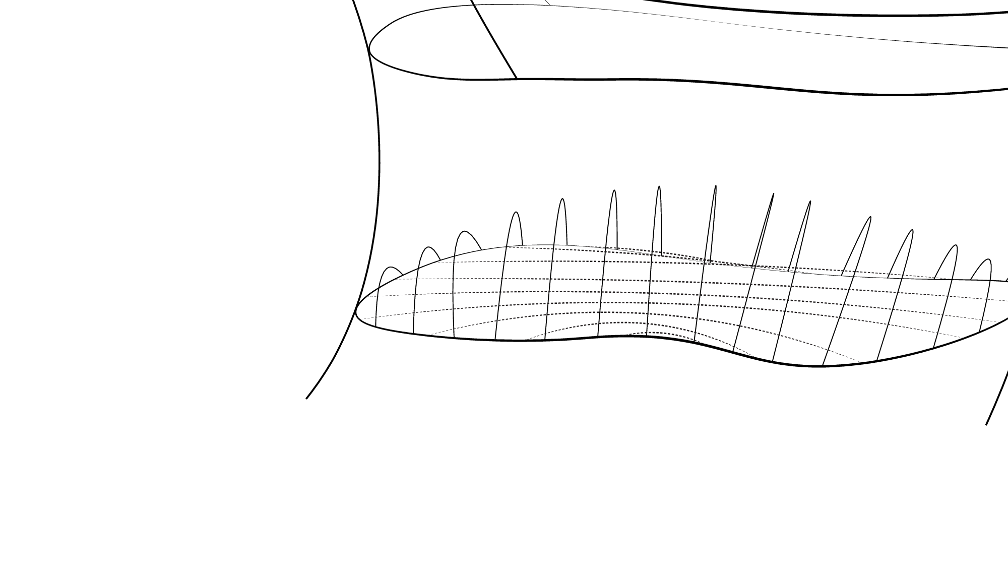
We can, however, repeat the same procedure for all different leaves . Here, is the time parameter on the holographic screen. The coordinates on different leaves can be defined from those on by following the integral curves of a vector field on the holographic screen which is orthogonal to every leaf. (Such a vector field was used [47] to prove that the area theorem of Refs. [17, 48] is local.)
The continuity assumption then implies that for each the hypersurfaces sweep the entire spacetime region inside the holographic screen, , as varies:66 6 In the case that the holographic screen is spacelike, it seems logically possible that for some does not sweep the entire spacetime. We do not consider such a possibility.
| (29) |
This in turn implies that for any bulk point inside the holographic screen, we can find the values of and for each , (, ), such that the corresponding HRT surface goes through (see Fig. 1). Therefore, by choosing
| (30) |
the point can be written as in Eq. (21).
We note that in general, for different need not be the same. And yet, the region giving each entanglement wedge is on a single leaf.
IV.2 Reconstructable Shadow
The construction described above does not apply if there is an entanglement shadow : a spacetime region which the HRT surfaces do not probe. This phenomenon occurs rather generally, for example in spacetimes with a conical deficit [49] or a dense star [50]. Here we show that a point may still be written as in Eq. (21) if certain conditions are met. An important point is that while an HRT surface is always outside the shadow, the other part of the boundary of the entanglement wedge can go into the shadow region.
Consider the future light cone of , which we define as the subset of covered by the set of future-directed light rays, , emanating from in all directions parameterized by angles . Similarly, we can consider the set of past-directed light rays , emanating from in all directions. Suppose all future (past) directed light rays escape the shadow region by the time the first future (past) directed light ray intersects the holographic screen (if at all), i.e. they all enter early enough.77 7 We assume that these light rays enter while their congruences are still expanding. This is generally true for small shadow regions. We now show that point can then be reconstructed as in Eq. (21). A sketch of the procedure is given in Fig. 2.

Let us take a point on the portion of in . We can then find an HRT surface, , that goes through , tangent to the light cone there, and anchored on some leaf of the holographic screen. An argument is the following. As in the previous subsection, we consider families of HRT surfaces anchored on ; see Eq. (28). In the previous subsection, we considered such sets , but now we consider an infinite number of sets parameterized by the angular coordinates on : . (The corresponding spatial region can be taken to enlarge from the point specified by toward its antipodal point as increases from to .) Because of the entanglement shadow, these surfaces, (), do not cover the entire interior achronal surface bounded by ; there will be some hole(s). However, by extending this to all possible leaves , for each will sweep the entire region outside the shadow:
| (31) |
This implies that we have a set of HRT surfaces parameterized by that all go through :
| (32) |
From these, we can choose one that is tangent to the light cone at because this imposes conditions on the parameters .
We therefore have the appropriate HRT surface for , which is anchored on leaf . There are two regions on this leaf that can be associated with , which are complement with each other on the leaf. We take the one such that the boundary of its entanglement wedge contains , and we call it . We then find that the intersection of the entanglement wedges of for all gives a region that is a subset of the causal future of and contains :
| (33) |
Repeating the same construction for the past light cone, we obtain the analogous region with . Since the intersection of and is just , we find that by taking
| (34) |
we can write in the form of Eq. (21). Note that each region or is on a single leaf.
We conclude that to reconstruct through Eq. (21), it is sufficient that all the future-directed and past-directed light rays emanating from reach outside the entanglement shadow early enough. This condition, however, appears too strong as a necessary condition for the reconstruction.
In general, the bulk portion of the boundary of an entanglement wedge consists of three elements: (i) the HRT surface, (ii) null surfaces generated by light rays emanating orthogonally from the HRT surface, and (iii) caustics developed by the congruence of these light rays. To reconstruct a point through Eq. (21), one of these elements must go through . For a point in an entanglement shadow, (i) is not available. In the construction above, we have used (ii). We can, however, also use (iii).
Consider a spatial region on a leaf. Suppose that is chosen such that a caustic developed by a congruence of past-directed light rays emanating from passes through . Suppose also that we can find such regions, (), which seems possible generically based on parameter counting. Then, the intersection of ,
| (35) |
forms a region which has a “tip” at . It therefore seems possible to find a region such that a caustic developed by a congruence of future-directed light rays emanating from passes through , and that
| (36) |
gives through Eq. (21); see Fig. 3. This would allow us to reconstruct without requiring that all the light rays emanating from reach outside the entanglement shadow.

In all the reconstruction procedures we could consider, however, it seems necessary that at least one future-directed and past-directed light ray from escapes the entanglement shadow region. We thus require this as a necessary condition for to be reconstructable. (This is, in fact, a very weak requirement. In every case we considered, we actually needed a stronger condition.)
IV.3 Non-reconstructable Shadow
The necessary condition described above has important implications. Suppose a black hole is formed in . After a sufficiently long time, the black hole becomes quasi-static. For any such black hole, HRT surfaces anchored on leaves cannot penetrate the horizon [51, 21]. The condition described above then implies that the interior of a quasi-static black hole cannot be reconstructed directly in the holographic theory.
Two comments are in order. First, the entanglement shadow around a black hole in general extends beyond the horizon (except for a large black hole in AdS) [50]. This region, however, is reconstructable as described in the previous subsection. Second, HRT surfaces may probe the interior of the event horizon shortly after a black hole is formed [52], which allows us to reconstruct the region as described in Section IV.1. After the black hole is stabilized, however, no HRT surface can penetrate the horizon (at least by any macroscopic distance). The interior of a stabilized black hole, therefore, still cannot be reconstructed.
We interpret this non-reconstructability to mean that in the given reference frame the black hole interior is not described in terms of local operators in semiclassical spacetime (at least a priori; see below). Suppose we (try to) represent a bulk point as in Eq. (21) with some . Let us call the element of on the latest (earliest) leaf () and the corresponding time parameter on the holographic screen (). Let us define as the smallest value of over the possible choices of :
| (37) |
The analyses in the previous subsections imply that for a reconstructable bulk point, is finite. On the other hand, for a non-reconstructable point, we may view that is infinite (as the relevant light ray fails to escape the shadow region in a finite time). This implies that using operators that probe (only) entanglement entropies between subregions, it takes an infinite time to resolve a point in the non-reconstructable region. In other words, the effective theory for the degrees of freedom represented by these operators describe physics in this region as a “vacuum degeneracy,” condensed in the energy interval of .
This strongly suggests that the description obtained in the holographic theory is that of a distant picture for the black hole. (Recall that it is the entanglement entropy structure between subregions that local bulk operators under consideration are mainly sensitive to.) This, however, does not necessarily mean that there can be no effective description that makes (a portion of) the interior spacetime manifest by appropriately rearranging degrees of freedom. Based on intuition from Ref. [24], and more recent analysis in Ref. [53], we expect that such a description—if any—cannot keep locality in all the original spacetime region (in particular, outside the causal patch of a single infalling geodesic). In fact, we expect that any such effective description is applicable only for a finite time, measured with respect to the degrees of freedom made local in this way, reflecting the fact that the corresponding spacetime has a singularity. The issue of the black hole interior will be discussed further in Section VI.
We finally present another example of spacetime with a non-reconstructable region: an isotropic AdS cosmology. Through a coordinate transformation, the interior of a future light cone in global AdS space can be written as an open FRW universe with the metric
| (38) |
Any small perturbation makes this universe end with a big-crunch collapse at some time (), so that
| (39) |
where the hypersurface is taken to be on . In Ref. [21], it was shown that HRT surfaces anchored to the AdS boundary cannot probe the region
| (40) |
where is the time at which becomes maximum. Since any future-directed light ray emanating from a point in this region hits the singularity, our criterion says that this region is not reconstructable. (The region is reconstructable as it is probed by HRT surfaces.)
In fact, it seems that any non-reconstructable region in realistic spacetimes is associated with a collapsing region (region in which time runs backwards in the language of Ref. [17]) whose future ends in a singularity. (We have excluded the region inside a past light cone in the isotropic AdS cosmology, which we consider “unrealistic,” analogous to the white hole region.) This may be viewed as a quantum gravity version of cosmic censorship, although the surface “hiding” a singularity, i.e. that dividing reconstructable and non-reconstructable regions, is not necessarily null here.
V Spacetime Is Non-Generic
We have discussed what description the holographic theory provides when a holographic state represents semiclassical spacetime. Here we discuss how such states are embedded in the holographic Hilbert space.
V.1 Holographic Encoding of Spacetime
Consider the holographic space of volume , which consists of cutoff-size cells containing degrees of freedom. If a state on this space (an element of ) represents a semiclassical spacetime (or more precisely a snapshot of it in the holographic theory), then the von Neumann entropy of a subregion is related to the area of the HRT surface as [11]
| (41) |
ignoring the bulk matter contribution, which does not play a role in the discussion below. Here, represents the volume of the object (often called the area for a codimension-two surface in spacetime).
Suppose we take an entanglement structure on implied by some semiclassical spacetime. Since any unitary transformation acting within a single cell does not change entanglement entropies between subregions, this allows us to have a set of states labeled by the group elements of
| (42) |
all having the same entanglement structure . We expect that some (but not necessarily all) of these states are microstates of the corresponding spacetime.
In general, we expect that is large because entanglement between different subregions is robust (only) when many degrees of freedom are involved; see, e.g., Eq. (19).88 8 Later, we consider perfect tensor network models, which do not a priori require large bond dimensions (which one might think are analogous to here). For small bond dimensions, however, perfect tensors are finely tuned: small perturbations would destroy their absolutely maximally entangled nature. Models with these tensors can be used (only) to simulate coarse-grained structures of the fundamental theory. For large bond dimensions, this issue of stability does not arise. In the case of AdS/CFT, i.e. where is the AdS length, is related to the ratio of to the bulk Planck length (which we restore here):
| (43) |
For more general spacetimes, which one may view as the case , the meaning of is not clear, but one possibility is
| (44) |
where and are the string length and the number of species in the low energy bulk effective theory, respectively. We then expect that is also large in this case.
The degrees of freedom in corresponding to the microstates of the spacetime may contain a large amount of information, especially for . Such information cannot be captured by entanglement between different subregions on . In Section IV.3, we have seen that semiclassical physics in a non-reconstructable region cannot be captured by entanglement entropies between subregions, so it is natural to conjecture that this physics (e.g. physics of the excitations of the stretched horizon) is encoded in these degrees of freedom. We might suspect that physics outside the holographic screen may also be encoded in these degrees of freedom. If this is true, the logarithmic dimension of the Hilbert space describing both the interior and exterior regions of the holographic screen is [10]. An alternative possibility is that the degrees of freedom describing the exterior region is not captured by those discussed here. (They may not even be arranged locally in any space.) In this case, the system we discuss here should be regarded as that responsible only for the interior region.
V.2 Semiclassical States Are Special
The number of independent states within the space of is . This implies that there can be up to independent microstates for the same semiclassical spacetime, within the uncertainties associated with the coarse-graining , although this does not mean that all, or even any, semiclassical spacetimes must have that many independent microstates.
If a semiclassical spacetime has independent microstates, however, it leads to the following puzzling situation.99 9 One might expect that given standard de Sitter entropy [54], the de Sitter FRW universe provides an example of such spacetime, with independent microstates. This is, however, not the case, since spacetime “disappears” in the de Sitter limit of the holographic FRW theory [20]. Suppose there are independent microstates () which all correspond to (a holographic snapshot of) a single semiclassical spacetime and hence have the same entanglement structure .1010 10 We expect this basis of microstates to be uncorrelated with the position space basis states in holographic space and take this to be the case. Suppose we take a superposition of such states
| (45) |
with comparable coefficients. Here, . If we compute the holographic entanglement entropy of this state in a subregion , we generally obtain
| (46) |
For small , where
| (47) |
we find
| (48) |
so that the second term (classical Shannon entropy) is of order , which is negligible compared with the first term (typically of order ). If we superpose a sufficiently large number of microstates with , however, the entanglement structure of , , can take a form unrelated with , since form (approximately) a basis of . Indeed, for a generic superposition with , we expect from Page’s argument [55] that to a high degree.
On the other hand, one might expect that the state still describes semiclassical spacetime , since it is simply a superposition of microstates that all describe the same semiclassical spacetime . If this were true, then we would find that a generic state describing spacetime , i.e. a generic state of the form of Eq. (45), has an entanglement structure that has nothing to do with . This would violate assumption (ii) in the introduction.
We are, therefore, led to the conclusion that if a semiclassical spacetime has independent microstates, then these states do not form a Hilbert space. In fact, the space of microstates for a fixed semiclassical spacetime is at most the space (see Eq. (42)), whose volume is tiny compared with that of :
| (49) |
In fact, the actual space of microstates can be smaller. Note that taken at face value, the space of microstates given by Eq. (49) is measure zero in . Our expressions, however, apply only at the leading order in , so we expect that the space has a nonzero “width” at subleading order in . This, however, does not affect our conclusion that an arbitrary superposition of the form of Eq. (45) cannot be interpreted as a semiclassical state representing .
If the microstates of a spacetime comprise the entire space, then what happens? We can use tensor network models to simulate this situation.1111 11 Strictly speaking, the models discussed in this and next subsections apply only to the situation in which the holographic space is approximately time independent, but we expect that the conclusions are more general, since the time independence does not play a particularly important role. For example, consider a tensor network obtained by contracting perfect tensors with some bulk legs left dangling. By varying the perfect tensor chosen at each node, while keeping the network structure unaltered, we can generate a class of quantum error correcting codes represented in the holographic space. This generates the code subspaces for all the geometry microstates satisfying the condition that for all . The semiclassical (logical) operators obtained in this way are state-dependent, because different semiclassical states in different code subspaces have nontrivial overlaps in the holographic Hilbert space. The same conclusion is obtained using random tensor networks, rather than perfect tensor networks.
A similar observation about state-dependence has been made recently in Ref. [39] which considered overlaps of code subspaces corresponding to different geometries realized in the same holographic space. On the other hand, our discussion here concerns microstates corresponding to the same semiclassical geometry, which does not require different matter configurations at the semiclassical level. The basic outcome for the purpose of the present discussion, however, is that the two situations can be treated similarly.1212 12 This is consonant with the picture of Refs. [40, 41, 56] that different microstates for the “same” spacetime (e.g. a single classical black hole) can/should actually be viewed as states with slightly different spacetimes (black holes with slightly different masses).
The fact that the space of microstates for a fixed semiclassical spacetime is bounded from above by () has an important implication. Consider a generic state in . In such a state, the entanglement entropy of a region is given by
| (50) |
where is defined by Eq. (47). This is because for a typical state, the reduced density matrix of a subsystem smaller than a half of the whole system is maximally mixed to a high degree [55]. If this state is interpreted through Eq. (41), we have
| (51) |
An essentially unique way in which this happens is that the HRT surface anchored to is itself (or , whichever is smaller). The corresponding geometry in then must have a horizon just inside the leaf, which serves as an extremal surface barrier. Since the description of the holographic theory is that of the exterior picture, this state does not have any semiclassical spacetime inside .1313 13 The relation in Eq. (51) can be obtained in a different way (only) if a leaf and the HRT surfaces can be mapped on an extremal surface using a (infinitely) large boost transformation; then the HRT surfaces lie on a null hypersurface associated with the leaf. Spacetime also disappears in this case [20]. (This indeed occurs in the de Sitter limit of flat FRW universes.)
We conclude that a generic state in the holographic Hilbert space does not represent a semiclassical spacetime inside the holographic screen. Specifically, if the initial state of a system is generic in and if the dynamics of the holographic theory is such that the state keeps being generic in throughout the evolution, where , then the system does not admit a semiclassical spacetime interpretation within the holographic screen. In this sense, we can say that bulk gravitational spacetime emerges only as a result of non-genericity of the state in the holographic Hilbert space.
We emphasize, though, that non-genericity here refers to that in the holographic Hilbert space without a constraint. In particular, our argument does not exclude the possibility that with a specification of an energy range which is sufficiently lower than the cutoff, semiclassical states are generic among the states in that energy range. This is indeed the case in standard AdS/CFT. Similarly, it is possible that imposing a constraint on some other quantity makes semiclassical states typical within the specified class. Further discussion on this issue is given in Ref. [20].
V.3 State-dependence and Many Microstates
We have learned that a semiclassical spacetime inside the holographic screen appears only as a result of non-genericity of the holographic state. We have also argued that if a semiclassical spacetime has independent microstates, then the semiclassical operators are state-dependent. This latter argument has been made by considering that the semiclassical microstates occupy the space. Here we show that the necessity of state-dependence for a spacetime having independent microstates is even more robust.
The smallest possible space containing independent microstates consists of discrete “axis” states (with some small “width” around them). In this case, all the different code subspaces can be exactly orthogonal:
| (52) |
where () represents the elements of the code subspace associated with microstate . One might then think that any semiclassical operator can be represented state-independently as
| (53) |
without any subtlety. Here, act “correctly” on elements of but annihilate all the other states:
| (54) |
Indeed, if these operators are represented in the whole holographic space , then there is no obstacle in defining them as in Eq. (54), so that we can build any semiclassical operator state-independently through Eq. (53).
However, an important feature—or rather a defining property—of semiclassical operators is that they are represented in multiple different regions in the holographic space . Unlike the case of measuring a standard physical object, in quantum gravity there is no large external environment in which information can be amplified, and hence the amplification must occur “internally” within the holographic degrees of freedom given by the system. The holographic theory achieves this by utilizing quantum error correction, amplifying information of entanglement entropies between the holographic degrees of freedom (which makes this information—the geometry—robust under operations in code subspaces). A consequence of this is that operators in code subspaces, i.e. semiclassical operators, are represented in multiple subregions on .
We now argue that the requirement of a semiclassical operator being represented redundantly on subregions of in the present setup prevents us from defining the operator in the form of Eq. (53) acting universally on all the microstates. To see this, we use models given by the stabilizer formalism, which describes a broad class of quantum error correcting codes. In this formalism, the logical states are those living in the simultaneous eigenspace of an abelian subgroup of the Pauli group. For physical qubits, the Pauli group is comprised of Pauli operators which are a tensor product of Pauli matrices: . For qudits of higher dimensions, this can be appropriately generalized.
We consider that the degrees of freedom of the holographic theory are physical qudits. Let be the physical (holographic) Hilbert space and be an abelian subgroup of the Pauli group, which we consider to be fixed. Then the states in the code subspace can be defined as
| (55) |
The group is called the stabilizer of the code. We regard this code subspace as the Hilbert space of the semiclassical theory built on one of the microstates. A class of operators that have particular significance are logical operators. These operators have nontrivial action on the states in the code subspace and are given by elements of the Pauli group that commute with but are not elements of .
Now, instead of Eq. (55), we could have chosen any other of the simultaneous eigenspaces (with eigenvalues not all ) to be our code subspace. These eigenspaces are orthogonal and completely cover the full physical Hilbert space; we say that they “tile” . We identify these eigenspaces to be code subspaces associated with microstates . In this setup, each code subspace has elements (), so that
| (56) |
and
| (57) |
It is, in fact, simple to build tensor network models realizing this framework. For example, we may consider perfect tensor networks discussed in the previous subsection; but instead of choosing an arbitrary perfect tensor at each node, we now choose a tensor from simultaneous eigenstates of some fixed stabilizer group. This leads to quantum error correcting codes that have a particular entanglement structure and correspond to discussed above.
The quantum error correcting nature of the codes allows us to represent a semiclassical operator for each microstate in various subregions in , which we denote by . Note that in general
| (58) |
although these operators act identically on states in their own code subspaces:
| (59) |
where do not depend on or possible choices of . We regard that the operators obtained in this way are essentially the only semiclassical operators. This realizes the situation in which the space of microstates consists of discrete basis states (with some possible small “widths”).
By construction, the operators all commute with the stabilizer generators
| (60) |
where are interpreted to be defined on the whole holographic space , acting trivially on . This implies that actions of these operators do not send a state out of the code subspace it belongs to
| (61) |
so that the matrix elements of these operators are nonzero only between states in the same code subspace
| (62) |
We also find that the matrix elements involving states and operators of different code subspaces have entries but only with the probability of :
| (63) |
where we have normalized operators such that nonvanishing in Eq. (59) are .
The property of Eq. (63) follows because the quantum error correcting code corresponding to each microstate can be viewed as a single large tensor having logical qudits and physical qudits as its indices. The set of tensors corresponding to all the microstates can then be viewed as the simultaneous eigenstates of some fixed (stabilizer) generators acting on all these indices. This structure guarantees that Eq. (63) is satisfied.1414 14 Instead of adopting the exact stabilizer formalism as we did here, we could use random tensor network models to simulate the setup in which the microstates comprise axis states. To do so, we can choose generic codes from those obtained by randomly varying the tensor at each node of a fixed network; these codes then approximately tile . In these models, essentially all the elements in the left-hand side of Eq. (63) are nonzero, but they are uniformly suppressed as . This does not change the conclusion of our analysis here.
We now see how the properties in Eqs. (61 – 63) prevents us from having state-independent semiclassical operators. In order for exactly state-independent semiclassical operators to be defined, must satisfy
| (64) |
at least for small values of . In this case, the operators represented in subregion
| (65) |
would become the direct sum form of Eq. (53) and act correctly on all possible states of the form
| (66) |
However, for , the conditions in Eq. (64) are not satisfied for all operators; see Eq. (63).
In fact, nonzero entries in Eq. (63) do not allow for even approximately state-independent operators. To see this, consider the matrix elements
| (67) |
where we have used Eq. (59) and . The first term is what we want, but the second term gives a much larger contribution , where the square root in the leftmost expression arises because of random phases. This implies that we cannot define state-independent semiclassical operators even approximately.
Note that the origin of the state-dependence is not the overlap between different code subspaces. In fact, different code subspaces are orthogonal, Eq. (52), in the present (extreme) setup of discrete microstates. Semiclassical operators, however, still must be defined state-dependently because of the requirement of being represented redundantly in the holographic space. We find that the necessity of state-dependence is robust in the holographic theory if there are independent microstates for a semiclassical spacetime.
We thus conclude either that semiclassical states are special or that bulk operators are state-dependent, in which case semiclassical states can be generic.
VI Black Hole Interior
We finally discuss the issue of the black hole interior within our framework. A simple description of the interior would arise if a portion of the holographic screen enters inside the black hole horizon. However, we find this is unlikely to occur in a realistic setup in which the second law of thermodynamics, , is obeyed. First, the holographic screen cannot approach close to the singularity, since then the area of the leaf would decrease in time, contradicting the assumption of . This leaves the possibility that a portion of a leaf enters the black hole and then exits or terminates. Even in this case, however, we would still encounter the strange situation where the portion of a leaf inside the black hole has a larger area than the corresponding part of the black hole horizon. We therefore assume that the holographic screen does not enter inside the black hole horizon (except possibly in transient periods), though a general proof is lacking.
This only leaves the possibility that the black hole interior can be described effectively by rearranging the degrees of freedom of the theory (which include the stretched horizon degrees of freedom identified in Section IV). Such a description would make approximate locality in a portion of the interior manifest at the cost of the local description in some other region (the complementarity picture [24]).1515 15 In AdS/CFT, this might be done along the lines of Refs. [28, 29]. We suspect that the requirement of the same interior region being represented redundantly, associated with amplification, might address the question of why the specific set of operators considered in Refs. [28, 29] has a special physical significance. We note that this rearrangement of the degrees of freedom would have a different nature than just changing the reference frame, e.g., by boosting the origin of a freely falling reference frame with respect to which the holographic screen is erected. In fact, we expect that any effective description of the black hole interior is applicable only for a finite time (measured with respect to the degrees of freedom made local) reflecting the existence of the singularity, while the reference frame change would give another description of the system which does not have such a restriction.
What about the arguments of Refs. [25, 26, 27] then, which seem to exclude even the possibility of this kind of (effective) description? These arguments can essentially be summarized into two classes:
-
Entanglement argument. Consider an outgoing mode localized in the zone, corresponding to a Hawking quanta just emitted from the stretched horizon. Unitarity requires this mode to be entangled with a mode representing Hawking radiation emitted earlier, while the smoothness of the horizon requires it to be entangled with the pair mode inside the horizon. These two cannot both be true because of monogamy of entanglement.
-
Typicality argument. Suppose we calculate the average of the number operator in the dual field theory over states having energies in a chosen range, with corresponding to an infalling mode in the bulk. The resulting number is at least of order unity, because one can choose a basis for these states such that they are all eigenstates of the number operator with corresponding to a mode localized in the zone (and because the expectation value of in any eigenstate of is at least of order unity). This implies that the expectation value of is of order unity or larger, giving firewalls, in a typical state in this energy range.
The former, entanglement argument was addressed in Refs. [40, 41]. At the level of a semiclassical description, the Bekenstein-Hawking entropy, , can be interpreted as the logarithm of the number of independent black hole states of masses between and , where can be taken naturally as the inverse of the Hawking emission timescale. Interpreted in terms of semiclassical operators, this information is distributed according to the thermodynamic entropy associated with the blue-shifted Hawking temperature. This implies that while most of the information is concentrated near the stretched horizon, it has some spread over the zone. In particular, an amount of information—which is an fraction of the full Bekenstein-Hawking entropy—is at the edge of the zone.
From the semiclassical viewpoint, Hawking emission is a process in which the black hole information (and energy), stored in spacetime, is converted into that of semiclassical excitations at the edge of the zone (more precisely, the region around the edge of the zone with the radial width of order the wavelength of emitted Hawking quanta). Note that in the semiclassical viewpoint it is natural that the process occurs in this particular region; it is where the two static geometries—the near horizon, Rindler-like space and asymptotic, Minkowski-like space—are “patched” to obtain the full geometry. This implies that it is incorrect to view that Hawking emission (and the associated information transfer) occurs through outgoing semiclassical excitations in the zone as envisioned in Refs. [25, 26, 27]. In fact, the transfer of energy and information must be viewed as occurring through the flux of negative energy and negative entropy, defined with respect to the static, Hartle-Hawking vacuum.
The typicality argument does not apply when semiclassical operators are given state-dependently [28, 29]. Moreover, if the black hole microstates comprise only a subset of the space spanned by the independent microstates, as contemplated in Section V.3, then the argument may become irrelevant because the black hole microstates would indeed be non-generic. If this is the case, then smooth black hole states would have to be selected dynamically.
Finally, the fact that the holographic screen does not enter the black hole may allow us to take the attitude that the black hole interior need not be described, since a measurement performed in the interior cannot be communicated to an external observer described directly in the holographic theory. Of course, what “happened inside” is encoded indirectly in the final Hawking radiation (and in the configuration of the stretched horizon degrees of freedom at intermediate stages), which can be described appropriately in the holographic theory.
Acknowledgements.
We thank Chris Akers, Venkatesa Chandrasekaran, Adrian Franco Rubio, Aitor Lewkowycz, Fabio Sanches, Arvin Shahbazi Moghaddam, and Sean Weinberg for discussions. This work was supported in part by the National Science Foundation under grants PHY-1521446, by MEXT KAKENHI Grant Number 15H05895, and by the Department of Energy (DOE), Office of Science, Office of High Energy Physics, under contract No. DE-AC02-05CH11231.Appendix A Reconstruction from a Single Leaf
In this appendix, we study what portion of the bulk can be reconstructed from a single leaf, i.e. by Eq. (21) with all on a single leaf. We refer to three types of spacetime regions discussed in Sections IV.1, IV.2, and IV.3 as non-shadow, reconstructable shadow, and non-reconstructable shadow regions, respectively.
| Single leaf | Multiple leaves | |
|---|---|---|
| Non-shadow | codimension- | codimension- |
| (codimension- for ) | ||
| Reconstructable shadow | none | codimension- |
| Non-reconstructable shadow | none | none |
Let us first consider a spacetime point in a non-shadow region. We show that generically a codimension- neighborhood of can be directly reconstructed from a single leaf . For this purpose, we consider a timelike geodesic, , that goes through at and stays in the non-shadow region. We then introduce a map from the coordinates, , parameterizing to as follows. For each , we consider a continuous family of HRT surfaces associated with subregions of which are taken to enlarge naturally from the point specified by toward its antipodal point. Generically, one of these HRT surfaces intersects with at some , which we take as the image of the map: . Now, we can choose so that and . The set satisfying is generally codimension- in the space of , hence there are many such which have an HRT surface passing through . This tells us that can be reconstructed from this single leaf. In addition, continuity suggests that some interval of is reconstructed from this leaf. Applying this argument for points outside of entanglement shadows tells us that a single leaf generally allows for the reconstruction of a codimension- region of the bulk.
Note that there is a case in which the above argument does not apply. Suppose the spacetime is time reflection symmetric with respect to , as in the case of a static system. Then all HRT surfaces anchored to live on the same bulk hypersurface corresponding to the reflection symmetric point. This therefore allows for reconstructing only a codimension- region. The situation for reconstructing non-shadow regions from a single leaf is summarized in the upper-left entry of Table 1.
We now prove that a single leaf cannot reconstruct any portion of an entanglement shadow. We will do so by contradiction. Suppose a point resides within an entanglement shadow but can be reconstructed by a single leaf, . Then there is a subregion of , , such that lies on the boundary of the entanglement wedge of . Now, suppose some subregion of , , has nonzero overlap with , i.e. is codimension- on the leaf. Then is codimension- in the bulk, and will not be sufficient to localize . Therefore, there must be some subregion of , , where and the boundary of intersects . However, from entanglement wedge nesting, , and thus it cannot be the case. Note that this is a result of subregion duality, which tells us that the only intersection of and is the HRT surface. This implies that multiple leaves are necessary to reconstruct bulk regions in entanglement shadows.
Table 1 gives a summary of directly reconstructable bulk regions from boundary states.
References
- [1] H. Ollivier, D. Poulin and W. H. Zurek, “Objective properties from subjective quantum states: environment as a witness,” Phys. Rev. Lett. 93, 220401 (2004) [arXiv:quant-ph/0307229].
- [2] R. Blume-Kohout and W. H. Zurek, “Quantum Darwinism: entanglement, branches, and the emergent classicality of redundantly stored quantum information,” Phys. Rev. A 73, 062310 (2006) [arXiv:quant-ph/0505031].
- [3] Y. Nomura, “Quantum mechanics, spacetime locality, and gravity,” Found. Phys. 43, 978 (2013) [arXiv:1110.4630 [hep-th]].
- [4] A. Almheiri, X. Dong and D. Harlow, “Bulk locality and quantum error correction in AdS/CFT,” JHEP 04, 163 (2015) [arXiv:1411.7041 [hep-th]].
- [5] F. Pastawski, B. Yoshida, D. Harlow and J. Preskill, “Holographic quantum error-correcting codes: toy models for the bulk/boundary correspondence,” JHEP 06, 149 (2015) [arXiv:1503.06237 [hep-th]].
- [6] D. Harlow, “The Ryu-Takayanagi formula from quantum error correction,” Commun. Math. Phys. 354, 865 (2017) [arXiv:1607.03901 [hep-th]].
- [7] S. Ryu and T. Takayanagi, “Holographic derivation of entanglement entropy from AdS/CFT,” Phys. Rev. Lett. 96, 181602 (2006) [hep-th/0603001].
- [8] V. E. Hubeny, M. Rangamani and T. Takayanagi, “A covariant holographic entanglement entropy proposal,” JHEP 07, 062 (2007) [arXiv:0705.0016 [hep-th]].
- [9] A. Lewkowycz and J. Maldacena, “Generalized gravitational entropy,” JHEP 08, 090 (2013) [arXiv:1304.4926 [hep-th]].
- [10] Y. Nomura, N. Salzetta, F. Sanches and S. J. Weinberg, “Toward a holographic theory for general spacetimes,” Phys. Rev. D 95, 086002 (2017) [arXiv:1611.02702 [hep-th]].
- [11] F. Sanches and S. J. Weinberg, “Holographic entanglement entropy conjecture for general spacetimes,” Phys. Rev. D 94, 084034 (2016) [arXiv:1603.05250 [hep-th]].
- [12] T. Faulkner, A. Lewkowycz and J. Maldacena, “Quantum corrections to holographic entanglement entropy,” JHEP 11, 074 (2013) [arXiv:1307.2892 [hep-th]].
- [13] N. Engelhardt and A. C. Wall, “Quantum extremal surfaces: holographic entanglement entropy beyond the classical regime,” JHEP 01, 073 (2015) [arXiv:1408.3203 [hep-th]].
- [14] P. Hayden, S. Nezami, X.-L. Qi, N. Thomas, M. Walter and Z. Yang, “Holographic duality from random tensor networks,” JHEP 11, 009 (2016) [arXiv:1601.01694 [hep-th]].
- [15] M. Miyaji and T. Takayanagi, “Surface/State correspondence as a generalized holography,” PTEP 2015, 073B03 (2015) [arXiv:1503.03542 [hep-th]].
- [16] F. Sanches and S. J. Weinberg, “Boundary dual of bulk local operators,” Phys. Rev. D 96, 026004 (2017) [arXiv:1703.07780 [hep-th]].
- [17] R. Bousso and N. Engelhardt, “New area law in general relativity,” Phys. Rev. Lett. 115, 081301 (2015) [arXiv:1504.07627 [hep-th]].
- [18] A. C. Wall, “Maximin surfaces, and the strong subadditivity of the covariant holographic entanglement entropy,” Class. Quant. Grav. 31, 225007 (2014) [arXiv:1211.3494 [hep-th]].
- [19] M. Headrick, V. E. Hubeny, A. Lawrence and M. Rangamani, “Causality & holographic entanglement entropy,” JHEP 12, 162 (2014) [arXiv:1408.6300 [hep-th]].
- [20] Y. Nomura, P. Rath and N. Salzetta, “Spacetime from unentanglement,” arXiv:1711.05263 [hep-th].
- [21] N. Engelhardt and A. C. Wall, “Extremal surface barriers,” JHEP 03, 068 (2014) [arXiv:1312.3699 [hep-th]].
- [22] D. L. Jafferis, A. Lewkowycz, J. Maldacena and S. J. Suh, “Relative entropy equals bulk relative entropy,” JHEP 06, 004 (2016) [arXiv:1512.06431 [hep-th]].
- [23] X. Dong, D. Harlow and A. C. Wall, “Reconstruction of bulk operators within the entanglement wedge in gauge-gravity duality,” Phys. Rev. Lett. 117, 021601 (2016) [arXiv:1601.05416 [hep-th]].
- [24] L. Susskind, L. Thorlacius and J. Uglum, “The stretched horizon and black hole complementarity,” Phys. Rev. D 48, 3743 (1993) [hep-th/9306069].
- [25] A. Almheiri, D. Marolf, J. Polchinski and J. Sully, “Black holes: complementarity or firewalls?,” JHEP 02, 062 (2013) [arXiv:1207.3123 [hep-th]].
- [26] A. Almheiri, D. Marolf, J. Polchinski, D. Stanford and J. Sully, “An apologia for firewalls,” JHEP 09, 018 (2013) [arXiv:1304.6483 [hep-th]].
- [27] D. Marolf and J. Polchinski, “Gauge/gravity duality and the black hole interior,” Phys. Rev. Lett. 111, 171301 (2013) [arXiv:1307.4706 [hep-th]].
- [28] K. Papadodimas and S. Raju, “State-dependent bulk-boundary maps and black hole complementarity,” Phys. Rev. D 89, 086010 (2014) [arXiv:1310.6335 [hep-th]].
- [29] K. Papadodimas and S. Raju, “Remarks on the necessity and implications of state-dependence in the black hole interior,” Phys. Rev. D 93, 084049 (2016) [arXiv:1503.08825 [hep-th]].
- [30] R. Bousso, “Holography in general space-times,” JHEP 06, 028 (1999) [hep-th/9906022].
- [31] Y. Nomura, “Physical theories, eternal inflation, and the quantum universe,” JHEP 11, 063 (2011) [arXiv:1104.2324 [hep-th]].
- [32] R. Bousso, “A covariant entropy conjecture,” JHEP 07, 004 (1999) [hep-th/9905177].
- [33] J. M. Maldacena, “Eternal black holes in anti-de Sitter,” JHEP 04, 021 (2003) [hep-th/0106112].
- [34] W. K. Wootters and W. H. Zurek, “A single quantum cannot be cloned,” Nature 299, 802 (1982).
- [35] L. G. Yaffe, “Large limits as classical mechanics,” Rev. Mod. Phys. 54, 407 (1982).
- [36] B. Swingle, “Entanglement renormalization and holography,” Phys. Rev. D 86, 065007 (2012) [arXiv:0905.1317 [cond-mat.str-el]].
- [37] Y. Nomura, N. Salzetta, F. Sanches and S. J. Weinberg, “Spacetime equals entanglement,” Phys. Lett. B 763, 370 (2016) [arXiv:1607.02508 [hep-th]].
- [38] D. L. Jafferis, “Bulk reconstruction and the Hartle-Hawking wavefunction,” arXiv:1703.01519 [hep-th].
- [39] X.-L. Qi, Z. Yang and Y.-Z. You, “Holographic coherent states from random tensor networks,” JHEP 08, 060 (2017) [arXiv:1703.06533 [hep-th]].
- [40] Y. Nomura, F. Sanches and S. J. Weinberg, “Black hole interior in quantum gravity,” Phys. Rev. Lett. 114, 201301 (2015) [arXiv:1412.7539 [hep-th]].
- [41] Y. Nomura, F. Sanches and S. J. Weinberg, “Relativeness in quantum gravity: limitations and frame dependence of semiclassical descriptions,” JHEP 04, 158 (2015) [arXiv:1412.7538 [hep-th]].
- [42] Y. Nomura and N. Salzetta, “Why firewalls need not exist,” Phys. Lett. B 761, 62 (2016) [arXiv:1602.07673 [hep-th]].
- [43] Y. Nomura, “A note on Boltzmann brains,” Phys. Lett. B 749, 514 (2015) [arXiv:1502.05401 [hep-th]].
- [44] K. K. Boddy, S. M. Carroll and J. Pollack, “De Sitter space without dynamical quantum fluctuations,” Found. Phys. 46, 702 (2016) [arXiv:1405.0298 [hep-th]].
- [45] M. Headrick and T. Takayanagi, “A holographic proof of the strong subadditivity of entanglement entropy,” Phys. Rev. D 76, 106013 (2007) [arXiv:0704.3719 [hep-th]].
- [46] D. Kabat and G. Lifschytz, “Local bulk physics from intersecting modular Hamiltonians,” JHEP 06, 120 (2017) [arXiv:1703.06523 [hep-th]].
- [47] F. Sanches and S. J. Weinberg, “Refinement of the Bousso-Engelhardt area law,” Phys. Rev. D 94, 021502 (2016) [arXiv:1604.04919 [hep-th]].
- [48] R. Bousso and N. Engelhardt, “Proof of a new area law in general relativity,” Phys. Rev. D 92, 044031 (2015) [arXiv:1504.07660 [gr-qc]].
- [49] V. Balasubramanian, B. D. Chowdhury, B. Czech and J. de Boer, “Entwinement and the emergence of spacetime,” JHEP 01, 048 (2015) [arXiv:1406.5859 [hep-th]].
- [50] B. Freivogel, R. A. Jefferson, L. Kabir, B. Mosk and I.-S. Yang, “Casting shadows on holographic reconstruction,” Phys. Rev. D 91, 086013 (2015) [arXiv:1412.5175 [hep-th]].
- [51] V. E. Hubeny, “Extremal surfaces as bulk probes in AdS/CFT,” JHEP 07, 093 (2012) [arXiv:1203.1044 [hep-th]].
- [52] V. E. Hubeny and H. Maxfield, “Holographic probes of collapsing black holes,” JHEP 03, 097 (2014) [arXiv:1312.6887 [hep-th]].
- [53] S. Raju, “Smooth causal patches for AdS black holes,” Phys. Rev. D 95, 126002 (2017) [arXiv:1604.03095 [hep-th]].
- [54] G. W. Gibbons and S. W. Hawking, “Cosmological event horizons, thermodynamics, and particle creation,” Phys. Rev. D 15, 2738 (1977).
- [55] D. N. Page, “Average entropy of a subsystem,” Phys. Rev. Lett. 71, 1291 (1993) [gr-qc/9305007].
- [56] Y. Nomura and S. J. Weinberg, “Black holes, entropies, and semiclassical spacetime in quantum gravity,” JHEP 10, 185 (2014) [arXiv:1406.1505 [hep-th]].