Hidden attractors on one path:
Glukhovsky-Dolzhansky, Lorenz, and Rabinovich systems

G. Chen Affiliation: City University of Hong Kong, Hong Kong SAR, China N.V. Kuznetsov Affiliation: Faculty of Mathematics and Mechanics, St. Petersburg State University, Peterhof, St. Petersburg, Russia Affiliation: Department of Mathematical Information Technology, University of Jyväskylä, Jyväskylä, Finland G.A. Leonov Affiliation: Faculty of Mathematics and Mechanics, St. Petersburg State University, Peterhof, St. Petersburg, Russia Affiliation: Institute of Problems of Mechanical Engineering RAS, Russia T.N. Mokaev Affiliation: Faculty of Mathematics and Mechanics, St. Petersburg State University, Peterhof, St. Petersburg, Russia

August 24, 2026

Abstract

In this report, by the numerical continuation method we visualize and connect hidden chaotic sets in the Glukhovsky-Dolzhansky, Lorenz and Rabinovich systems using a certain path in the parameter space of a Lorenz-like system.

I Introduction

In 1963, meteorologist Edward Lorenz suggested an approximate mathematical model (the Lorenz system) for the Rayleigh-Bénard convection and discovered numerically a chaotic attractor in this model [1]. This discovery stimulated rapid development of the chaos theory, numerical methods for attractor investigation, and till now has received a great deal of attention from different fields [2, 3, 4, 5, 6, 7]. The Lorenz system gave rise to various generalizations, e.g. Lorenz-like systems, some of which are also simplified mathematical models of physical phenomena. In this paper, we consider the following Lorenz-like system

\begin{cases}\dot{x}$ = $-\sigma(x-y)-ayz\\ \dot{y}$ = $rx-y-xz\\ \dot{z}$ = $-bz+xy,\end{cases}

(1)

where parameters $r$ , $\sigma$ , $b$ are positive and $a$ is real. System (1) with

a=0

(2)

coincides with the classical Lorenz system.

Consider

b=1,\qquad a>0,\qquad\sigma>ar.

(3)

Then by the following linear transformation (see, e.g., [8]):

(x,y,z)\rightarrow\bigg(x,\frac{\zeta}{\sigma-ar},r-\frac{\zeta}{\sigma-ar}\,y\bigg),

(4)

system (1) is transformed to the Glukhovsky-Dolzhansky system [9]:

\begin{cases}\dot{x}$ = $-\sigma x+\zeta z+\alpha yz\\ \dot{y}$ = $\rho-y-xz\\ \dot{z}$ = $-z+xy,\end{cases}

(5)

where

\zeta>0,\quad\rho=\frac{r(\sigma-ar)}{\zeta}>0,\quad\alpha=\frac{\zeta^{2}a}{(\sigma-ar)^{2}}>0.

(6)

The Glukhovsky-Dolzhansky system describes the convective fluid motion inside a rotating ellipsoidal cavity.

If we set

a<0,\qquad\sigma=-ar,

(7)

then after the linear transformation (see, e.g., [8]):

(x,y,z)\rightarrow\bigg(\nu_{1}^{-1}\,y,\nu_{1}^{-1}\nu_{2}^{-1}h\,x,\nu_{1}^{-1}\nu_{2}^{-1}h\,z)\bigg),\quad t\to\nu_{1}\,t

with positive $\nu_{1},\nu_{2},h$ , we obtain the Rabinovich system [10, 11], describing the interaction of three resonantly coupled waves, two of which being parametrically excited:

\begin{cases}\dot{x}$ = $hy-\nu_{1}x-yz,\\ \dot{y}$ = $hx-\nu_{2}y+xz,\\ \dot{z}$ = $-z+xy,\end{cases}

(8)

where

\sigma=\nu_{1}^{-1}\nu_{2},\,b=\nu_{1}^{-1},\,a=-\nu_{2}^{2}h^{-2},\,r=\nu_{1}^{-1}\nu_{2}^{-1}h^{2}.

(9)

Hereinafter, the Lorenz, Glukhovsky-Dolzhansky, and Rabinovich systems are studied in the framework of system (1) under the corresponding assumptions on parameters ((2), (3), or (7)), respectively. For the considered assumptions on parameters, if $r<1$ , then (1) has a unique¹¹ 1 In general, system (1) can possess up to five equilibria [8]. equilibrium ${\bf\rm S_{0}}=(0,0,0)$ , which is globally asymptotically Lyapunov stable [8, 12]. If $r>1$ , then system (1) has three equilibria: ${\bf\rm S_{0}}=(0,0,0)$ and

{\bf\rm S_{\pm}}=(\pm x_{1},\,\pm y_{1},\,z_{1}).

(10)

Here,

x_{1}=\frac{\sigma b\sqrt{\xi}}{\sigma b+a\xi},\quad y_{1}=\sqrt{\xi},\quad z_{1}=\frac{\sigma\xi}{\sigma b+a\xi},

and

\xi=\frac{\sigma b}{2a^{2}}\left[a(r-2)-\sigma+\sqrt{(\sigma-ar)^{2}+4a\sigma}\right].

The stability of equilibria $S_{\pm}$ of system (1) depends on the parameters $r$ , $\sigma$ , $a$ and $b$ .

Lemma 1 (see, e.g. [13]).

For a certain $\sigma>2$ , the equilibria $S_{\pm}$ of system (1) with (3) (and, thus, of Glukhovsky-Dolzhansky system (5)) are stable if and only if the following condition holds:

$\displaystyle a^{2}\sigma^{2}(\sigma-2)r^{3}$	$\displaystyle-a\left(2\sigma^{4}-4\sigma^{3}-3a\sigma^{2}+4a\sigma+4a\right)r^{2}+$	(11)
	$\displaystyle+\sigma^{2}\left(\sigma^{3}+2(3a-1)\sigma^{2}-8a\sigma+8a\right)r-$
	$\displaystyle-\sigma^{3}\left(\sigma^{3}+4\sigma^{2}-16a\right)<0.$

Lemma 2 (see, e.g. [14]).

The equilibria $S_{\pm}$ of system (1) with (7) (and, thus, of the Rabinovich system (8)) are stable if and only if one of the following conditions holds:

(i)

$0\leq\,ar+1\,<\frac{2r}{r-\sqrt{r(r-1)}}$ ,
(ii)

$ar+1<0$ , $b>b_{\rm cr}=\frac{4a(r-1)(ar+1)\sqrt{r(r-1)}+(ar-1)^{3}}{(ar+1)^{2}-4ar^{2}}.$

The particular interest in the considered Lorenz-like systems is due to the existence of chaotic attractors in their phase spaces. In the next section, we will present the definition of attractor from analytical and numerical perspectives.

II Attractors of dynamical systems

II.1 Attractors of dynamical systems

Consider system (1) as an autonomous differential equation in a general form:

\dot{u}=f({u}),\qquad

(12)

where $u=(x,y,z)\in\mathbb{R}^{3}$ , and the continuously differentiable vector-function $f:\mathbb{R}^{3}\to\mathbb{R}^{3}$ may represent the right-hand side of system (1). Define by ${u}(t,{u}_{0})$ a solution of (12) such that ${u}(0,{u}_{0})={u}_{0}$ . For system (12), a bounded closed invariant set K is

(i)

a (local) attractor if it is a minimal locally attractive set (i.e., $\lim_{t\to+\infty}{\rm dist}(K,{u}(t,{u}_{0}))=0$ for all ${u_{0}}\in K(\varepsilon)$ , where $K(\varepsilon)$ is a certain $\varepsilon$ -neighborhood of set $K$ ),
(ii)

a global attractor if it is a minimal globally attractive set (i.e., $\lim_{t\to+\infty}{\rm dist}(K,{u}(t,{u}_{0}))=0$ for all ${u_{0}}\in\mathbb{R}^{n}$ ),

where ${\rm dist}(K,{u})=\inf_{{v}\in K}||{v}-{u}||$ is the distance from the point ${u}\in\mathbb{R}^{3}$ to the set $K\subset\mathbb{R}^{3}$ (see, e.g. [13]).

Note that system (1) is dissipative in the sense that it possesses a bounded convex absorbing set [8, 13]

\mathcal{B}=\left\{(x,y,z)\in\mathbb{R}^{3}\penalty\ |\penalty\ V(x,y,z)\leq\frac{b(\sigma+\delta r)^{2}}{2c(a+\delta)}\right\},

(13)

where $V(u)=V(x,y,z)=x^{2}+\delta y^{2}+(a+\delta)\left(z-\frac{\sigma+\delta r}{a+\delta}\right)^{2}$ , $\delta$ is an arbitrary positive number such that $a+\delta>0$ and $c=\min(\sigma,1,\frac{b}{2})$ . Thus, solutions of (12) exist for $t\in[0,+\infty)$ and system (1) possesses a global attractor [15, 13], which contains the set of equilibria and can be constructed as $\cap_{\tau>0}\overline{\cup_{t\geq\tau}\varphi^{t}\left(\mathcal{B}\right)}$ .

Computational errors (caused by finite precision arithmetic and numerical integration of differential equations) and sensitivity to initial conditions allow one to get a reliable visualization of a chaotic attractor by only one pseudo-trajectory computed on a sufficiently large time interval. For that, one needs to choose an initial point in attractor’s basin of attraction and observe how the trajectory starting from this initial point after a transient process visualizes the attractor. Thus, from a computational point of view, it is natural to suggest the following classification of attractors, based on the simplicity of finding the basin of attraction in the phase space.

Definition.

[16, 17, 18, 13] An attractor is called a self-excited attractor if its basin of attraction intersects with any open neighborhood of a stationary state (an equilibrium); otherwise, it is called a hidden attractor.

Remark.

Sustained chaos is often (almost) indistinguishable numerically from transient chaos (transient chaotic set in the phase space), which can nevertheless persist for a long time. Similar to the above definition, in general, a chaotic set can be called hidden if it does not involve and attract trajectories from a small vicinities of stationary states; otherwise, it is called self-excited.

For a self-excited attractor, its basin of attraction is connected with an unstable equilibrium and, therefore, self-excited attractors can be localized numerically by the standard computational procedure in which after a transient process a trajectory, started in a neighborhood of an unstable equilibrium (e.g., from a point of its unstable manifold), is attracted to the state of oscillation and then traces it. Thus, self-excited attractors can be easily visualized (see, e.g. the classical Lorenz, Rossler, and Hennon attractors can be visualized by a trajectory from a vicinity of unstable zero equilibrium).

For a hidden attractor, its basin of attraction is not connected with equilibria, and, thus, the search and visualization of hidden attractors in the phase space may be a challenging task. Hidden attractors are attractors in the systems without equilibria (see, e.g. rotating electromechanical systems with Sommerfeld effect described in 1902 [19, 20]), and in the systems with only one stable equilibrium (see, e.g. counterexamples [21, 18] to the Aizerman’s (1949) and Kalman’s (1957) conjectures on the monostability of nonlinear control systems [22, 23]). One of the first related problems is the second part of Hilbert’s 16th problem (1900) [24] on the number and mutual disposition of limit cycles in two-dimensional polynomial systems where nested limit cycles (a special case of multistability and coexistence of attractors) exhibit hidden periodic oscillations (see, e.g., [25, 26, 18]). The classification of attractors as being hidden or self-excited was introduced by G. Leonov and N. Kuznetsov in connection with the discovery of the first hidden Chua attractor [27, 16, 17, 28, 29] and has captured much attention of scientists from around the world (see, e.g. [30, 31, 32, 33, 34, 35, 36, 37, 38, 39, 40, 41, 42, 43, 44, 45, 46, 47, 48]).

II.2 Hidden attractor localization via numerical continuation method

One of the effective methods for numerical localization of hidden attractors in multidimensional dynamical systems is based on the homotopy and numerical continuation method (NCM). The idea is to construct a sequence of similar systems such that for the first (starting) system the initial point for numerical computation of oscillating solution (starting oscillation) can be obtained analytically. Thus, it is often possible to consider the starting system with self-excited starting oscillation; then the transformation of this starting oscillation in the phase space is tracked numerically while passing from one system to another; the last system corresponds to the system in which a hidden attractor is searched.

For studying the scenario of transition to chaos, we consider system (12) with $f(u)=f(u,\lambda)$ , where $\lambda\in\Lambda\subset\mathbb{R}^{d}$ is a vector of parameters, whose variation in the parameter space $\Lambda$ determines the scenario. Let $\lambda_{\rm end}\in\Lambda$ define a point corresponding to the system, where a hidden attractor is searched. Choose a point $\lambda_{\rm begin}\in\Lambda$ such that we can analytically or numerically localize a certain nontrivial (oscillating) attractor $\mathcal{A}^{1}$ in system (12) with $\lambda=\lambda_{\rm begin}$ (e.g., one can consider an initial self-excited attractor defined by a trajectory ${u}^{1}(t)$ numerically integrated on a sufficiently large time interval $t\in[0,T]$ with initial point ${u}^{1}(0)$ in the vicinity of an unstable equilibrium). Consider a path²² 2 In the simplest case, when $d=1$ , the path is a line segment. in the parameter space $\Lambda$ , i.e. a continuous function $\gamma\penalty\ :\penalty\ [0,\,1]\to\Lambda$ , for which $\gamma(0)=\lambda_{\rm begin}$ and $\gamma(1)=\lambda_{\rm end}$ , and a sequence of points $\{\lambda^{j}\}_{j=1}^{k}$ on the path, where $\lambda^{1}=\lambda_{\rm begin}$ , $\lambda^{k}=\lambda_{\rm end}$ , such that the distance between $\lambda^{j}$ and $\lambda^{j+1}$ is sufficiently small. On each next step of the procedure, the initial point for a trajectory to be integrated is chosen as the last point of the trajectory integrated on the previous step: ${u}^{j+1}(0)={u}^{j}(T)$ . Following this procedure and sequentially increasing $j$ , two alternatives are possible: the points of $\mathcal{A}^{j}$ are in the basin of attraction of attractor $\mathcal{A}^{j+1}$ , or while passing from system (12) with $\lambda=\lambda^{j}$ to system (12) with $\lambda=\lambda^{j+1}$ , a loss of stability bifurcation is observed and attractor $\mathcal{A}^{j}$ vanishes. If, while changing $\lambda$ from $\lambda_{\rm begin}$ to $\lambda_{\rm end}$ , there is no loss of stability bifurcation of the considered attractors, then a hidden attractor for $\lambda^{k}=\lambda_{\rm end}$ (at the end of the procedure) is localized.

Classical attractors obtained in the Lorenz, Rabinovich, and Glukhovsky-Dolzhansky systems are self-excited, each can be visualized easily by a trajectory from a small vicinity of one of the unstable equilibria (see [1], [10], [9], respectively).

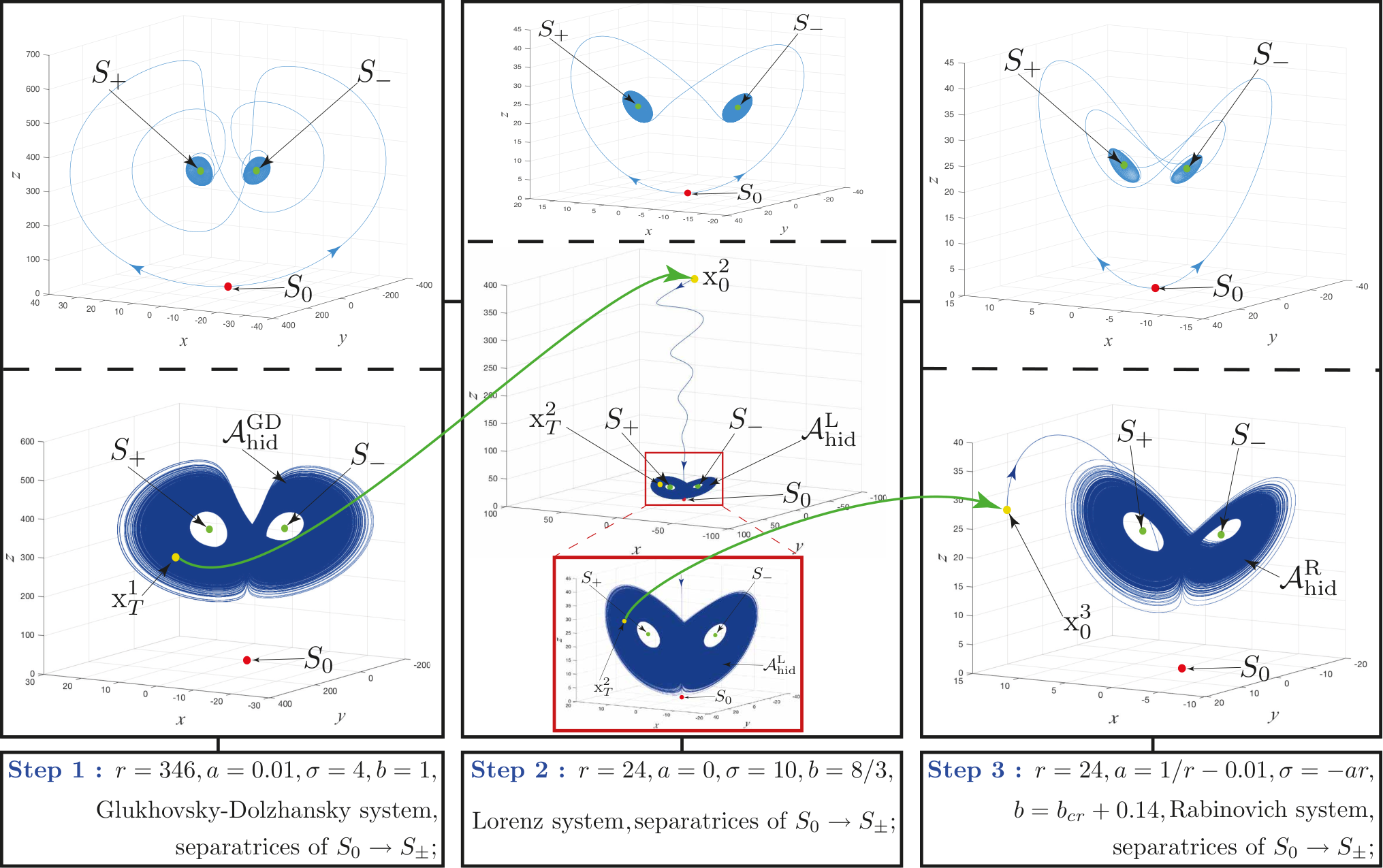
Recently, hidden attractors were discovered in the Glukhovsky-Dolzhansky system (5) for $\sigma=4$ (see [49, 13]) and in the Rabinovich system (see [14]) by numerical continuation method. For $\sigma=10$ , $b=8/3$ and $r=24$ in the Lorenz system, there exists a hidden bounded chaotic set (similar to the classical Lorenz attractor), which is numerically indistinguishable from sustained chaos since it persists for a very long time (see corresponding discussions in [50, 51]). Our aim here is to find a continuous path in the parameter space of system (1) that connects the above hidden chaotic set in the Lorenz system with the hidden Glukhovsky-Dolzhansky and Rabinovich attractors.

Figure 1: Path

P_{\rm GD}^{\,1}\to P_{\rm GD}^{\,2}\to P_{\rm GD}^{\,3}

in parameters plane

(a,r)

for localization of hidden GD attractor,

\sigma=4

;

(\bullet)

P_{\rm GD}^{\,1}(0.01,338)

: self-excited attractor with respect to

S_{0}

S_{\pm}

;

(\bullet)

P_{\rm GD}^{\,2}(0.01,342)

: self-excited attractor with respect to

S_{0}

;

(\bullet)

P_{\rm GD}^{\,3}(0.01,346)

: hidden attractor. Stability domain is defined according to inequality (11).

Refer to caption — Figure 2: Localization of hidden chaotic attractor (purple) in Glukhovsky-Dolzhansky systems defined by equations (1) and (3) using numerical continuation method. Here, trajectories ${\rm x}^{i}(t)=(x^{i}(t),y^{i}(t),z^{i}(t)$ (blue) are defined on the time interval $[0,T]$ ( $T=10^{1}$ ) and initial point on the $(i+1)$ -th iteration (yellow) is defined as ${\rm x}_{0}^{i+1}:={\rm x}_{T}^{i}$ (light green arrows), where ${\rm x}_{T}^{i}={\rm x}^{i}(T)$ is the final point (yellow). Outgoing separatrices of unstable zero equilibrium tend to two symmetric stable equilibria.

III Localization of hidden attractors on one path

In this experiment for system (1), we consider three sets of parameters: $P_{\rm GD}\,\left(r=346,\,a=0.01,\,\sigma=4,\,b=1\right)$ (for the Glukhovsky-Dolzhansky system — GD), $P_{\rm L}\,\left(r=24,\,a=0,\,\sigma=10,\,b=8/3\right)$ (for the Lorenz system — L), and $P_{\rm R}\,\left(r=24,\,a=-1/r-0.01,\,\sigma=-ar,\,b=b_{\rm cr}+0.14\right)$ (for the Rabinovich system — R). Here, we change the parameters in such a way that hidden Glukhovsky-Dolzhansky and Rabinovich attractors are located not too close to the unstable zero equilibrium so as to avoid a situation that numerically integrated trajectory persists for a long time and then falls on an unstable manifold of the unstable zero equilibrium, then leaves the transient chaotic set, and finally tends to one of the stable equilibria (see e.g. the corresponding discussion on the Lorenz system in [50]).

Hidden chaotic attractor in the Glukhovsky-Dolzhansky system with $P_{\rm GD}\,\left(r=346,\,a=0.01,\,\sigma=4,\,b=1\right)$ can be obtained from a self-excited attractor by numerical continuation method [49, 13]. See the corresponding path in the space of parameters in Fig. 1 and the localization procedure in Fig. 2.

These sets of parameters define three points, $P_{\rm GD}$ , $P_{\rm L}$ and $P_{\rm R}$ , in the 4D parameter space $(r,\,a,\,\sigma,\,b)$ . Consider two line segments, $P_{\rm GD}\rightarrow P_{\rm L}$ and $P_{\rm L}\rightarrow P_{\rm R}$ , defining two parts of the path in the continuation procedure. Choose the partition of the line segments into $N_{\rm st}=10$ parts and define intermediate values of parameters as follows: $P_{\rm GD\to L}^{i}=P_{\rm GD}+\frac{i}{N_{\rm st}}(P_{\rm L}-P_{\rm GD})$ and $P_{\rm L\to R}^{i}=P_{\rm L}+\frac{i}{N_{\rm st}}(P_{\rm R}-P_{\rm L})$ , where $i=1,\ldots,N_{\rm st}$ . Initial points for trajectories of system (1) that define hidden chaotic sets are presented in Table 1. At each iteration of the procedure, a chaotic attractor (defined by the trajectory in the phase space of system (1)) is computed. The last computed point of the trajectory at the previous step is used as the initial point for computation at the next step.

Table 1: Initial point

(x_{0},\,y_{0},\,z_{0})

and time interval

[0,\penalty\ T]

of numerical integration for each part of the path.

Path	$(x_{0},\,y_{0},\,z_{0})$	$T$
${\rm GD\to L}$	$(10.64,\,60.78,\,390)$	$10^{4}$
${\rm L\to R}$	$(0.2,\,0.2,\,0.35)$	$1.1\cdot 10^{4}$

By this procedure, starting from the hidden Glukhovsky-Dolzhansky attractor it is possible to localize numerically hidden chaotic sets in the Lorenz and Rabinovich systems. For the considered parameters, the trajectories, starting in small neighborhoods of unstable zero equilibrium, are not attracted by the computed chaotic set, and the outgoing separatrices of unstable zero equilibrium tend to two symmetric stable equilibria. Thus, the computed chaotic sets are hidden according to the above classification.

Remark.

The path and its partition are chosen such that during the procedure the obtained intermediate attractors are self-excited (equilibria $S_{\pm}$ are unstable) and the basin of attraction of the attractor at the current step intersects with the attractor obtained on the previous step.

Hereinafter, it is reasonable to try to increase the length of the step (i.e. decrease the number of the steps) in the continuation procedure, but we may face the situation where the basin of attraction of the current attractor does not intersect the previous attractor, or intersects it only partially. In this case, the result of the procedure depends on the time interval of the numerical integration of the trajectory.

All numerical experiments were performed in MATLAB R2016b using standard procedures for numerical ODE integration.

IV Conclusion

In this report, by means of the numerical continuation method we localize hidden chaotic sets on one path: from the Glukhovsky-Dolzhansky system through the Lorenz system to the Rabinovich system. This helps better understanding of hidden chaotic attractors and their relationships.

Acknowledgement

This work was supported by the Russian Science Foundation (project 14-21-00041).

References

[1] E. N. Lorenz, Deterministic nonperiodic flow, J. Atmos. Sci. 20 (2) (1963) 130–141.
[2] S. Celikovsky, A. Vanecek, Bilinear systems and chaos, Kybernetika 30 (1994) 403–424.
[3] C. Li, J. C. Sprott, W. Thio, Linearization of the Lorenz system, Physics Letters A 379 (10) (2015) 888–893.
[4] E. J. Doedel, B. Krauskopf, H. M. Osinga, Global organization of phase space in the transition to chaos in the Lorenz system, Nonlinearity 28 (11) (2015) R113.
[5] G. Leonov, N. Kuznetsov, On differences and similarities in the analysis of Lorenz, Chen, and Lu systems, Applied Mathematics and Computation 256 (2015) 334–343. doi:10.1016/j.amc.2014.12.132.
[6] G. Leonov, N. Kuznetsov, N. Korzhemanova, D. Kusakin, Lyapunov dimension formula for the global attractor of the Lorenz system, Communications in Nonlinear Science and Numerical Simulation 41 (2016) 84–103. doi:10.1016/j.cnsns.2016.04.032.
[7] J. Čermák, L. Nechvátal, The Routh–Hurwitz conditions of fractional type in stability analysis of the Lorenz dynamical system, Nonlinear Dynamics 87 (2) (2017) 939–954.
[8] G. A. Leonov, V. A. Boichenko, Lyapunov’s direct method in the estimation of the Hausdorff dimension of attractors, Acta Applicandae Mathematicae 26 (1) (1992) 1–60.
[9] A. B. Glukhovsky, F. V. Dolzhansky, Three component models of convection in a rotating fluid, Izv. Acad. Sci. USSR, Atmos. Oceanic Phys. 16 (1980) 311–318.
[10] M. I. Rabinovich, Stochastic autooscillations and turbulence, Uspehi Physicheskih Nauk 125 (1) (1978) 123–168.
[11] A. S. Pikovski, M. I. Rabinovich, V. Y. Trakhtengerts, Onset of stochasticity in decay confinement of parametric instability, Sov. Phys. JETP 47 (1978) 715–719.
[12] V. A. Boichenko, G. A. Leonov, V. Reitmann, Dimension Theory for Ordinary Differential Equations, Teubner, Stuttgart, 2005.
[13] G. Leonov, N. Kuznetsov, T. Mokaev, Homoclinic orbits, and self-excited and hidden attractors in a Lorenz-like system describing convective fluid motion, Eur. Phys. J. Special Topics 224 (8) (2015) 1421–1458. doi:10.1140/epjst/e2015-02470-3.
[14] N. Kuznetsov, G. Leonov, T. Mokaev, S. Seledzhi, Hidden attractor in the Rabinovich system, Chua circuits and PLL, AIP Conference Proceedings 1738 (1), art. num. 210008.
[15] I. Chueshov, Introduction to the Theory of Infinite-dimensional Dissipative Systems, Electronic library of mathematics, ACTA, 2002.
[16] N. Kuznetsov, G. Leonov, V. Vagaitsev, Analytical-numerical method for attractor localization of generalized Chua’s system, IFAC Proceedings Volumes 43 (11) (2010) 29–33. doi:10.3182/20100826-3-TR-4016.00009.
[17] G. Leonov, N. Kuznetsov, V. Vagaitsev, Localization of hidden Chua’s attractors, Physics Letters A 375 (23) (2011) 2230–2233. doi:10.1016/j.physleta.2011.04.037.
[18] G. Leonov, N. Kuznetsov, Hidden attractors in dynamical systems. From hidden oscillations in Hilbert-Kolmogorov, Aizerman, and Kalman problems to hidden chaotic attractors in Chua circuits, International Journal of Bifurcation and Chaos 23 (1), art. no. 1330002. doi:10.1142/S0218127413300024.
[19] A. Sommerfeld, Beitrage zum dynamischen ausbau der festigkeitslehre, Zeitschrift des Vereins deutscher Ingenieure 46 (1902) 391–394.
[20] M. Kiseleva, N. Kuznetsov, G. Leonov, Hidden attractors in electromechanical systems with and without equilibria, IFAC-PapersOnLine 49 (14) (2016) 51–55. doi:10.1016/j.ifacol.2016.07.975.
[21] G. Leonov, N. Kuznetsov, Algorithms for searching for hidden oscillations in the Aizerman and Kalman problems, Doklady Mathematics 84 (1) (2011) 475–481. doi:10.1134/S1064562411040120.
[22] M. A. Aizerman, On a problem concerning the stability in the large of dynamical systems, Uspekhi Mat. Nauk (in Russian) 4 (1949) 187–188.
[23] R. E. Kalman, Physical and mathematical mechanisms of instability in nonlinear automatic control systems, Transactions of ASME 79 (3) (1957) 553–566.
[24] D. Hilbert, Mathematical problems., Bull. Amer. Math. Soc. (8) (1901-1902) 437–479.
[25] N. N. Bautin, On the number of limit cycles generated on varying the coefficients from a focus or centre type equilibrium state, Doklady Akademii Nauk SSSR (in Russian) 24 (7) (1939) 668–671.
[26] N. Kuznetsov, O. Kuznetsova, G. Leonov, Visualization of four normal size limit cycles in two-dimensional polynomial quadratic system, Differential equations and dynamical systems 21 (1-2) (2013) 29–34. doi:10.1007/s12591-012-0118-6.
[27] G. Leonov, N. Kuznetsov, Localization of hidden oscillations in dynamical systems (plenary lecture), in: 4th International Scientific Conference on Physics and Control, 2009. http://www.math.spbu.ru/user/leonov/publications/2009-PhysCon-Leonov-plenary-hidden-oscillations.pdf#page=21
[28] G. Leonov, N. Kuznetsov, V. Vagaitsev, Hidden attractor in smooth Chua systems, Physica D: Nonlinear Phenomena 241 (18) (2012) 1482–1486. doi:10.1016/j.physd.2012.05.016.
[29] N. Kuznetsov, O. Kuznetsova, G. Leonov, V. Vagaitsev, Analytical-numerical localization of hidden attractor in electrical Chua’s circuit, Lecture Notes in Electrical Engineering 174 (4) (2013) 149–158. doi:10.1007/978-3-642-31353-0\_11.
[30] Q. Li, H. Zeng, X.-S. Yang, On hidden twin attractors and bifurcation in the Chua’s circuit, Nonlinear Dynamics 77 (1-2) (2014) 255–266.
[31] I. Burkin, N. Khien, Analytical-numerical methods of finding hidden oscillations in multidimensional dynamical systems, Differential Equations 50 (13) (2014) 1695–1717.
[32] C. Li, J. C. Sprott, Coexisting hidden attractors in a 4-D simplified Lorenz system, International Journal of Bifurcation and Chaos 24 (03), art. num. 1450034. doi:10.1142/S0218127414500345.
[33] G. Chen, Chaotic systems with any number of equilibria and their hidden attractors, in: 4th IFAC Conference on Analysis and Control of Chaotic Systems (plenary lecture), 2015, http://www.ee.cityu.edu.hk/~gchen/pdf/CHEN_IFAC2015.pdf.
[34] Z. Zhusubaliyev, E. Mosekilde, A. Churilov, A. Medvedev, Multistability and hidden attractors in an impulsive Goodwin oscillator with time delay, European Physical Journal: Special Topics 224 (8) (2015) 1519–1539.
[35] A. Kuznetsov, S. Kuznetsov, E. Mosekilde, N. Stankevich, Co-existing hidden attractors in a radio-physical oscillator system, Journal of Physics A: Mathematical and Theoretical 48 (2015) 125101.
[36] M. Chen, M. Li, Q. Yu, B. Bao, Q. Xu, J. Wang, Dynamics of self-excited attractors and hidden attractors in generalized memristor-based Chua’s circuit, Nonlinear Dynamics 81 (2015) 215–226.
[37] V. Semenov, I. Korneev, P. Arinushkin, G. Strelkova, T. Vadivasova, V. Anishchenko, Numerical and experimental studies of attractors in memristor-based Chua’s oscillator with a line of equilibria. Noise-induced effects, European Physical Journal: Special Topics 224 (8) (2015) 1553–1561.
[38] V.-T. Pham, F. Rahma, M. Frasca, L. Fortuna, Dynamics and synchronization of a novel hyperchaotic system without equilibrium, International Journal of Bifurcation and Chaos 24 (06), art. num. 1450087.
[39] M. Borah, B. K. Roy, Hidden attractor dynamics of a novel non-equilibrium fractional-order chaotic system and its synchronisation control, in: 2017 Indian Control Conference (ICC), 2017, pp. 450–455.
[40] T. Menacer, R. Lozi, L. Chua, Hidden bifurcations in the multispiral Chua attractor, International Journal of Bifurcation and Chaos 26 (14), art. num. 1630039.
[41] M. Messias, A. Reinol, On the formation of hidden chaotic attractors and nested invariant tori in the sprott a system, Nonlinear Dynamics 88 (2) (2017) 807–821.
[42] I. Zelinka, Evolutionary identification of hidden chaotic attractors, Engineering Applications of Artificial Intelligence 50 (2016) 159–167.
[43] M.-F. Danca, N. Kuznetsov, G. Chen, Unusual dynamics and hidden attractors of the Rabinovich–Fabrikant system, Nonlinear Dynamics 88 (2017) 791–805. doi:10.1007/s11071-016-3276-1.
[44] M.-F. Danca, Hidden transient chaotic attractors of Rabinovich–Fabrikant system, Nonlinear Dynamics 86 (2) (2016) 1263–1270.
[45] Z. Wei, V.-T. Pham, T. Kapitaniak, Z. Wang, Bifurcation analysis and circuit realization for multiple-delayed Wang–Chen system with hidden chaotic attractors, Nonlinear Dynamics 85 (3) (2016) 1635–1650.
[46] V.-T. Pham, C. Volos, S. Jafari, S. Vaidyanathan, T. Kapitaniak, X. Wang, A chaotic system with different families of hidden attractors, International Journal of Bifurcation and Chaos 26 (08) (2016) 1650139.
[47] S. Jafari, V.-T. Pham, S. Golpayegani, M. Moghtadaei, S. Kingni, The relationship between chaotic maps and some chaotic systems with hidden attractors, Int. J. Bifurcat. Chaos 26 (13), art. num. 1650211.
[48] D. Dudkowski, S. Jafari, T. Kapitaniak, N. Kuznetsov, G. Leonov, A. Prasad, Hidden attractors in dynamical systems, Physics Reports 637 (2016) 1–50. doi:10.1016/j.physrep.2016.05.002.
[49] G. Leonov, N. Kuznetsov, T. Mokaev, Hidden attractor and homoclinic orbit in Lorenz-like system describing convective fluid motion in rotating cavity, Communications in Nonlinear Science and Numerical Simulation 28 (2015) 166–174. doi:10.1016/j.cnsns.2015.04.007.
[50] J. Yorke, J. Yorke, Metastable chaos: the transition to sustained chaotic behavior in the Lorenz model, Journal of Statistical Physics 21 (263-277) (1979) 27–32.
[51] Q. Yuan, F.-Y. Yang, L. Wang, A note on hidden transient chaos in the Lorenz system, International Journal of Nonlinear Sciences and Numerical Simulation(accepted).

Listing 1: Numerical visualization of chaotic sets in the Glukhovsky-Dolzhansky, Lorenz and Rabinovich systems. plotAttractors.m – plot GD, Lorenz and Rabinovich hidden attractors.

⬇

1 function plotAttractors

2 % GD parameters (r, a > 0, sigma > a*r, b = 1) and initial point:

3 r_GD = 346; a_GD = 0.01; b_GD = 1; sigma_GD = 4; trajGD_0 = [10, 60, 390];

4 % Lorenz paramters (r, b, sigma > 0, a = 0) and initial point:

5 r_L = 24; a_L = 0; b_L = 8/3; sigma_L = 10; trajL_0 = [0.2, 0.2, 0.35];

6 % Rabinovich parameters (r, b > 0, a < 0, sigma = -a * r) and initial point:

7 r_R = 24; a_R = -1 / r_R - 0.01; b_cr = (4 * a_R * (r_R - 1) * (a_R * r_R + 1) * ...

8 sqrt(r_R * (r_R - 1)) + (a_R * r_R - 1)^3) / ((a_R * r_R + 1)^2 - 4 * a_R * r_R^2);

9 b_R = b_cr + 0.14; sigma_R = - a_R * r_R; trajR_0 = [-2.4, 3.6, 23.6];

10 % Integration time:

11 tEnd = 1e4;

12 % Plot GD, Lorenz and Rabinovich attractors:

13 figure(1); plot3d(trajGD_0, tEnd, r_GD, a_GD, b_GD, sigma_GD);

14 figure(2); plot3d(trajL_0, tEnd, r_L, a_L, b_L, sigma_L);

15 figure(3); plot3d(trajR_0, tEnd, r_R, a_R, b_R, sigma_R);

16 % Generalized Lorenz system:

17 function out = genLorSys(t, x, r, a, b, sigma)

18 out = zeros(3,1);

19 out(1) = - sigma * x(1) + sigma * x(2) - a * x(2) * x(3);

20 out(2) = r * x(1) - x(2) - x(1) * x(3);

21 out(3) = x(1) * x(2) - b * x(3);

22 end

23 % Attractor plotting routine:

24 function plot3d(traj0, tEnd, r, a, b, sigma)

25 % ODE solver settings:

26 acc = 1e-8; RelTol = acc; AbsTol = acc; InitialStep = acc/10;

27 solverOptions = odeset(’RelTol’, RelTol, ’AbsTol’, AbsTol, ...

28 ’InitialStep’, InitialStep, ’NormControl’, ’on’);

29 % Integration of the trajectory:

30 [~, traj] = ode45(@(t, x) genLorSys(t, x, r, a, b, sigma), ...

31 [0, tEnd], traj0, solverOptions);

32 % Equilibria:

33 S0 = [0 0 0];

35 if a == 0

36 S12XY = sqrt(b*(r-1)); S12Z = r-1;

37 S1 = [S12XY, S12XY, S12Z]; S2 = [-S12XY, -S12XY, S12Z];

38 else

39 XSI = (sigma*b)/(2*a^2)*(a*(r-2)-sigma + sqrt((a*r-sigma)^2+4*a*sigma));

40 S12X1 = (sigma*b*sqrt(XSI))/(sigma*b + a*XSI);

41 S12Y1 = sqrt(XSI); S12Z1 = (sigma*XSI)/(sigma*b + a*XSI);

42 S1 = [S12X1, S12Y1, S12Z1]; S2 = [-S12X1, -S12Y1, S12Z1];

43 end

45 plot3(S0(1), S0(2), S0(3), ’.’, ’markersize’, 15, ’Color’, ’red’); hold on;

46 text(0, 0, 0,’S_0’,’fontsize’, 18);

48 plot3(S1(1), S1(2), S1(3), ’.’, ’markersize’, 20, ’Color’, ’green’);

49 text(S1(1), S1(2), S1(3),’S_1’,’fontsize’, 18);

51 plot3(S2(1), S2(2), S2(3), ’.’, ’markersize’, 20, ’Color’, ’green’);

52 text(S2(1), S2(2), S2(3),’S_2’,’fontsize’, 18);

54 plot3(traj(:, 1), traj(:, 2), traj(:, 3), ’Color’, ’blue’); hold off;

56 xlabel(’x’); ylabel(’y’); zlabel(’z’);

57 grid on; axis auto; view(3);

58 end

59 end

Hidden attractors on one path: Glukhovsky-Dolzhansky, Lorenz, and Rabinovich systems

Abstract

I Introduction

Lemma 1 (see, e.g. [13]).

Lemma 2 (see, e.g. [14]).

II Attractors of dynamical systems

II.1 Attractors of dynamical systems

Definition.

Remark.

II.2 Hidden attractor localization via numerical continuation method

III Localization of hidden attractors on one path

Remark.

IV Conclusion

Acknowledgement

References

Hidden attractors on one path:
Glukhovsky-Dolzhansky, Lorenz, and Rabinovich systems