Kira – A Feynman Integral Reduction Program
Abstract
In this article, we present a new implementation of the Laporta algorithm to reduce scalar multi-loop integrals—appearing in quantum field theoretic calculations—to a set of master integrals. We extend existing approaches by using an additional algorithm based on modular arithmetic to remove linearly dependent equations from the system of equations arising from integration-by-parts and Lorentz identities. Furthermore, the algebraic manipulations required in the back substitution are optimized. We describe in detail the implementation as well as the usage of the program. In addition, we show benchmarks for concrete examples and compare the performance to Reduze 2 and FIRE 5. In our benchmarks we find that Kira is highly competitive with these existing tools.
FR-PHENO-2017-14
TCDMATH 18–02
PROGRAM SUMMARY
Manuscript Title: Kira – A Feynman Integral Reduction Program
Authors: P. Maierhöfer, J. Usovitsch and P. Uwer
Program title: Kira
Licensing provisions: GPLv3 or later
Programming language: C++
Computer(s) for which the program has been designed: desktop PC, compute nodes/workstations
Operating system(s) for which the program has been designed: Linux 64bit
RAM required to execute with typical data: depends on the complexity of the problem, from few MB up to a few hundred GB, or even
more in complicated cases.
Has the code been vectorized or parallelized?: yes
Number of processors used: any number of cores
Supplementary material: this article, examples
Keywords: Feynman diagrams, multi-loop Feynman integrals, dimensional regularization, Laporta algorithm, modular
arithmetic, computer algebra
CPC Library Classification: 4.4 Feynman diagrams, 4.8 Linear Equations and Matrices, 5 Computer Algebra
External routines/libraries used: Fermat [1], gateToFermat [2], GiNaC [3,4], yaml-cpp [5], zlib [6] and SQLite3 [7]
Nature of problem:
The reduction of Feynman integrals to master integrals leads in
general to a system of equations which contains redundant, i.e. linearly
dependent, equations. In particular, for multi-scale problems, the algebraic
manipulation of these redundant equations can lead to a substantial increase in
runtime and memory consumption without affecting the results.
Solution method:
The program identifies linearly dependent relations based on modular
arithmetic with the help of an algorithm presented in Ref. [8]. Afterwards the program brings a linearly independent system of equations in a triangular form. Furthermore, the algebraic manipulations required in the back substitution are optimized.
Restrictions: the CPU time and the available RAM
Running time: minutes to weeks, depending on the complexity of the problem
References:
[1] R. H. Lewis, Computer Algebra System Fermat, https://home.bway.net/lewis/.
[2] M. Tentioukov, gateToFermat, http://science.sander.su/FLink.htm.
[3] C. W. Bauer, A. Frink, and R. Kreckel, Introduction to the GiNaC framework for symbolic computation within the C++ programming language, J. Symb. Comput. 33 (2000) 1, arXiv:cs/0004015 [cs-sc].
[4] J. Vollinga, GiNaC: Symbolic computation with C++, Nucl. Instrum. Meth. A559 (2006) 282-284, arXiv:hep-ph/0510057 [hep-ph].
[5] YAML, YAML Ain’t Markup Language, http://yaml.org.
[6] J.-L. Gailly and M. Adler, ZLIB, http://zlib.net.
[7] SQLite, SQLite3, version: 3.14.2, https://www.sqlite.org.
[8] P. Kant, Finding Linear Dependencies in Integration-By-Parts Equations: A Monte Carlo Approach, Comput. Phys. Commun. 185 (2014) 1473-1476, arXiv:1309.7287 [hep-ph].
1 Introduction
The steadily increasing experimental precision reached in current collider experiments like ATLAS and CMS requires on the theory side the evaluation of higher order corrections in the perturbative expansion. While the computation of next-to-leading order (NLO) corrections is well established today, the same level of maturity has not yet been reached for next-to-next-to-leading order (NNLO) calculations, although tremendous progress has been made in the last few years, see for example [1, 2, 3, 4, 5, 6, 7, 8, 9, 10, 11, 12, 13, 14, 15, 16, 17] for an incomplete list of recent calculations.
One major bottleneck in the evaluation of multi-loop amplitudes is the computation of the occurring Feynman integrals. The application of Feynman rules leads in general to tensor integrals. All Feynman integrals may be calculated directly. This approach is worked out in [18, 19, 20]. However, in most applications it is advantageous to reduce the tensor integrals to scalar integrals. Because of integration-by-parts [21, 22] and Lorentz [23] identities these integrals are not independent and can be expressed in terms of a small set of so-called master integrals. The integration-by-parts and Lorentz identities relate integrals with different powers of the propagators. Combining these relations algebraically, ‘ladder-operators’ to reduce the powers of the propagators in form of a recursion can be constructed. In practice, this procedure is however highly non-trivial and cumbersome.
Alternatively, the integration-by-parts and Lorentz relations can be evaluated for integer (instead of algebraic) powers of the propagators. Using different integer values for the different powers as seeds, a system of equations can be set up. Solving this system leads to a reduction to master integrals. This is the essence of the Laporta algorithm [24]. Since the integral reduction is a crucial step in the analytic evaluation of multi-loop amplitudes, various publicly available implementations of the Laporta algorithm exist: AIR [25], FIRE [26, 27, 28] and Reduze [29, 30]. Applying these programs to state-of-the-art calculations depending on several mass scales (internal/external particle masses and scalar products of external momenta) the required runtime and the memory consumption may put severe limits in practical applications.
In this article we present an optimized implementation of the Laporta algorithm with the aim to extend the frontier of achievable reductions to more mass scales. Generating the system of equations using different input seeds leads in general to a system of equations which contains redundant, i.e. linearly dependent, equations. In particular, for multi-scale problems, the algebraic manipulation of these redundant equations can lead to a substantial increase in runtime and memory consumption without affecting the results. In Ref. [31] a method has been presented to eliminate the linearly dependent equations using only fixed-size integer arithmetic instead of computationally intense algebraic manipulations. The main idea is to replace the different mass scales occurring in the problem by integer numbers over a finite field and perform a Gauss type elimination afterwards to identify dependent equations. Besides the elimination of redundant equations, this procedure allows us to identify the master integrals before or even without performing the actual reduction, a task for which otherwise dedicated algorithms or computer programs are required, e.g. [32, 33]. Furthermore, the handling of the algebraic integral coefficients occurring in the reduction tables is improved. We find that these modifications lead to a substantial improvement in performance, in particular, when multi-scale problems are studied. In addition, since Kira uses input very similar to the one required by Reduze 2, our implementation can also be used to perform independent cross checks of results generated with Reduze 2.
The outline of this article is as follows. To introduce the notation we briefly review in section 2 some basic aspects of multi-loop Feynman integrals. In section 3 we describe our implementation of the Laporta algorithm. Section 4 gives detailed information on the required prerequisites and how to install Kira. In section 5 we illustrate the usage with a simple example. In addition, information on various options to tune the reduction is provided. Section 6 presents some benchmarks. More precisely, three double box topologies with non-vanishing internal and external masses are reduced and the required runtime is reported. As reference we also present the runtime required using the program Reduze 2 [29, 30]. We finally close with a conclusion in section 7.
2 Preliminaries
To fix the notation used in this work we start with a brief review of multi-loop integrals as encountered in perturbative calculations in quantum field theory. Applying within a concrete model the Feynman rules to calculate scattering matrix elements leads to multi-loop tensor integrals of the form
| (1) |
The momenta denote the linearly independent external momenta. (We consider a scattering amplitude with external momenta/legs, however, because of momentum conservation only momenta are independent.) The momenta are the loop momenta which are not fixed through momentum conservation at each vertex. With we denote the number of propagators of which are independent. The inverse propagators are of the form
| (2) |
with being a linear combination of the momenta and and denoting the masses of the corresponding virtual particles. Within dimensional regularization denotes the dimension of space-time. As usual is used to regularize infra-red and ultraviolet divergences. Using projectors or a Feynman/Schwinger type parametrization the multi-loop tensor integrals can be reduced to scalar multi-loop integrals. The Feynman/Schwinger type parametrization will introduce scalar integrals with shifted dimensions and indices. The projectors will generate scalar integrals with auxiliary propagators which represent irreducible scalar propagators. The required number of auxiliary propagators is easily calculated. The number of scalar products involving the loop-momenta is given by
| (3) |
However, scalar products can be expressed in terms of linear combinations of the propagators. The number of auxiliary propagators is thus given by . The occurring integrals can thus be cast in the form
| (4) |
where the powers of the auxiliary propagators (i.e. ) may only take non-positive values. Note that the auxiliary propagators are not uniquely fixed. They are constrained only by the requirement that together with the first propagators all scalar products involving the loop momenta are expressible as linear combinations of the propagators. As a short hand notation we collect the indices into an dimensional vector .
Integration-by-parts and Lorentz-invariance identities:
Performing the reduction of the tensor integrals to scalar integrals outlined above leads in general to a large number of scalar integrals. However, these integrals are not independent. So called Integration-By-Parts (IBP) identities [21, 22] and Lorentz-Invariance (LI) [23] lead to linear relations between them. As a consequence the large number of scalar integrals can be reduced to a smaller set of master integrals, which serve as a basis to express all other scalar integrals. To be more specific the IBP equations follow from
| (5) |
with for and for . For a fixed vector the possible choices for and lead to IBP equations relating integrals with indices shifted by one unit to each other.
The LI equations follow from
| (6) |
Contracting this equation with all possible antisymmetric combinations of the form
| (7) |
leads to equations between integrals with shifted indices. To reduce the large number of scalar integrals to the master integrals there are essentially two different strategies. One method is to combine the LI and IBP relations to construct ‘ladder-operators’ for the individual propagators. A recursive application of these ladder-operators can then be used to reduce all integrals to the master integrals. However, in practice this approach suffers from the fact that the construction of the ladder-operators is non-trivial and often involves some handwork. For recent progress in this direction we refer to Refs. [27, 34, 35]. In the second approach the IBP- and LI-equations are applied to integer instead of algebraic . Making different choices for which are often called seeds a huge system of equations can be built up. Using different seeds leads in general to relations between different (unknown) scalar integrals. However, it turns out that the number of relations grows faster than the number of unknown integrals. Making the system big enough all required scalar integrals can be reduced to the master integrals by applying a Gauss type elimination algorithm. This is the essence of the Laporta approach first described in Ref. [24]. Alternative ways of using IBP identities for integral reduction have been explored e.g. in [36, 37]
Sectors and sub-sectors:
In practical applications it turns out that the system of equations typically shows some block structure. Since respecting this structure in the reduction may be beneficial it is useful to introduce the notion of sectors and sub-sectors. For a given scalar integral the related sector is defined as the set of integrals for which the subset of propagators occurring with positive powers is the same. For each we define a vector where the are set to one if and zero otherwise,
| (8) |
where is the Heaviside step function. All scalar integrals within one sector lead to the same . The scalar integral for which is called the corner integral of the sector. To uniquely label a sector we may identify the as the components of a binary representation of a sector id ,
| (9) |
The total number of possible sectors is given by . The number of different propagators appearing in the denominator of any integral of a sector is given by
| (10) |
Furthermore, we define the vector of positive propagator powers, , which is obtained from by removing all non-positive indices (preserving the order), and analogously the vector of negative propagator powers, . Within a sector the sum of all positive powers of the propagators and the negative sum of all non-positive powers constitute a measure for the complexity of an integral. It is thus convenient to define
| (11) |
Identification of trivial sectors:
Within dimensional regularization, scaleless integrals are consistently set to zero. In Ref. [38] it is shown that if the corner integral of a given sector is zero, all other integrals in this sector are zero, too. Accordingly, such a sector is called a trivial sector or a zero sector. To identify zero sectors, we employ the algorithm presented in Ref. [34]. The algorithm is based on the Feynman parameter representation of Feynman integrals,
| (12) |
with , and the Symanzik polynomials and , which are multivariate polynomials in the . To identify zero sectors, the function
| (13) |
is considered. If the equation
| (14) |
has a -independent solution for the corresponding sector is trivial. Identifying zero sectors in an early stage of the reduction procedure can greatly simplify the reduction.
Symmetry relations between integrals:
Another class of relations between Feynman integrals which are usually not covered by IBP and LI identities is given by symmetry relations. A simple example which exhibits such a symmetry is the one-loop bubble integral
| (15) |
which obeys the symmetry relation
| (16) |
corresponding to the shift
| (17) |
of the loop momentum . In general, symmetries can be derived from loop momentum shifts
| (18) |
and may also involve permutations of external momenta which leave the Mandelstam variables invariant. Such a transformation conveys a symmetry if applying it to an integral with only non-negative powers results in an integral where is a permutation of . Applying it to an integral which contains negative powers results in a linear combination of integrals. By employing such symmetry relations the number of independent integrals can be reduced, resulting in a smaller set of master integrals. Symmetries which relate integrals within the same sector to each other are commonly referred to as sector symmetries. Those which relate different sectors of the same or of different topologies to each other are referred to as sector mappings. Furthermore, in certain cases symmetries exist which apply only to integrals without negative propagator powers, because the relation can not be represented in terms of loop momentum shifts and external momentum permutations.
The sector mappings and sector symmetries are identified by applying the equation (13) to each corner integral. If the function in equation (13) is equal for two different corner integrals after a permutation of Feynman parameters and kinematic invariants then the two considered corner integrals exhibit a symmetry relation described above.
Kira can handle several topologies in a single run. By exploiting mappings between equivalent sectors of different topologies, a common set of linearly independent master integrals for the entire set of topologies will be found.
3 Laporta Algorithm – Implementation
In the Laporta algorithm the IBP, LI and symmetry relations are applied to a chosen set of integrals as defined in Eq. (4) to generate a linear homogeneous system of equations with the integrals as unknowns [24]. In the implementation presented in this article we use the C++ library GiNaC [39, 40] to perform the necessary algebraic manipulations. The set of integrals is constrained by
| (19) |
where and are defined in Eq. (11). , , and are user-defined values which control the set of seed integrals for which equations are generated. The integrals outside the interval limits which may be generated by applying IBP- and LI-relations to the seeds are called auxiliary integrals. The rank of the system of equations is always smaller than the number of different unknowns in the system. The goal of the Laporta reduction is to find a representation of all the seed integrals in terms of a small set of independent integrals, the so called master integrals. In practical applications only the master integrals are needed to be calculated by means of analytic or numeric algorithms since all other integrals appearing in the calculation can be expressed as linear combinations of them. In the following we present some implementation details of the reduction algorithm within Kira.
3.1 Ordering of integrals and equations
Ordering of the Integrals:
To define an order on the integrals, in Kira each integral is represented as a list of integer numbers , where represents the topology, is the sector id, the sum of positive indices in (Eq. (11)), the negative sum of negative indices (Eq. (11)), the vector of non-positive indices and the vector of positive indices. Note that may contain zeros. The integrals are then ordered lexicographically with respect to . Integrals which compare larger in this sense are regarded as more complicated.
Ordering of the Equations:
The ordering of the integrals is used to define a (pre)order of the equations. Kira represents each equation as a list of integrals , including the coefficients of the integrals,
| (20) |
The integrals within each list are ordered in descending order, i.e. for . The first integral in each equation is thus the most complicated one which appears in it and it serves as a natural first criterion for the complexity of the equation. While this is in principle sufficient to make the reduction algorithm work, it is convenient to add further criteria to impose an order of equations with the same most complicated integral. As the second criterion we choose the length of the equation, followed by the remaining integrals. I.e. the equations are ordered lexicographically with respect to:
| (21) |
The system of equations is thus represented as an ordered list of equations
| (22) |
where denotes the -th equation and if .
Note that this defines a total preorder on the equations rather than a total order, because it does not take into account the coefficients. Hence, equations which contain the same set of integrals are regarded as equally complex, even if they are not just multiples of each other.
3.2 Reduction procedure
3.2.1 Selection of linearly independent equations
In large systems of IBP equations it has been observed that a quite large fraction of the equations are linearly dependent, i.e. these equations can be removed from the system without affecting the solution. Given that the algebraic manipulations of the integral coefficients involve multivariate rational functions in the kinematic invariants and the dimension it is highly desirable to avoid any superfluous calculations involving linearly dependent equations. This is important both to prevent expression swell at intermediate steps and to avoid unnecessary time consuming algebraic simplifications of the integral coefficients when different equations are combined.
An algorithm to identify linearly dependent relations based on modular arithmetic has been presented in Ref. [31] together with an implementation in the computer program ICE. To our knowledge, the application of modular techniques, which are well-known in mathematics [41], to solve systems of IBP equations was discussed in Ref. [42]. Instead of ICE, Kira uses pyRed to identify redundant equations. pyRed is a C++ port of a component of an unpublished integral reduction framework originally written in Python. It differs in two major ways from the algorithm proposed in Ref. [31]. First, by using larger prime numbers in the modular arithmetic (and optionally arrays of finite integers as coefficients), the “Monte Carlo approach” is avoided. I.e. only a single run is required to obtain a reliable result. Second, a variant of the Gaussian elimination algorithm is chosen which exploits the sparsity of the system of IBP equations.
Each equation of the system is a linear combination of integrals with polynomial or rational coefficients. In the first step, pyRed maps all coefficients to a finite integer field, which is defined by a (large) prime number . The required algebraic operations are defined modulo . In particular, because is prime, the multiplicative inverse of each finite integer is guaranteed to exist and can be calculated by solving the equation for by the extended Euclidean algorithm or by modular exponentiation [43]. Numeric implementations of the former tend to be a bit more efficient than binary modular exponentiation. All variables in the coefficients, i.e. external (Mandelstam) invariants, masses and the dimension are substituted by pseudo-random numbers . Operations on finite integers are of constant complexity, i.e. the time for such an operation does not depend on the complexity of the original rational function.
The equations in the system are ordered as described in section 3.1. The forward elimination11 1 Forward and backward elimination refer to the two major steps in the algorithm to bring a matrix into diagonal form. In the forward elimination the upper triangle representation is achieved. In the following backward elimination the diagonal form is achieved by working in the opposite direction. is then performed as follows. For each equation in the system, substitute all previous equations in order of descending complexity. By this procedure, the sparsity of the system is retained to a large degree, whereas this would not be the case in the standard Gaussian elimination. The computational complexity of Gaussian elimination on a dense system of size is of . This also holds in the case of sparse systems which become dense in intermediate steps due to an inconvenient choice of the forward elimination algorithm. With our algorithm, the size of equations is largely independent of the system size, i.e. of , which reduces the complexity of the entire algorithm to . Note that we do not perform pivoting apart from the initial ordering of the equations, thus avoiding the additional computational cost of a pivoting operation. For optional usage we also implemented a forward elimination algorithm with the pivoting of Ref. [31]. For the price of drastically inferior scaling behaviour and memory consumption in pyRed this may in some cases lead to a better choice of independent equations in the sense that the following reduction steps in Kira are more efficient.
It is sufficient to just perform the forward elimination to identify redundant equations. However, we chose to perform the backward elimination by default as well. This operation is computationally cheap and it comes with two advantages. First, it allows us to extract the set of master integrals already at this stage. Second, it allows us to trace insertions of equations down to a full reduction in such a way, that we can extract a subsystem of equations which may be significantly smaller than the original system, but will suffice to fully reduce all integrals of a user-specified list.
Note that it is in principle possible to reconstruct rational functions from finite fields (see Ref. [41]). This was discussed in the context of Feynman integral reduction in Refs. [42] and [44]. A private implementation for single scale reduction problems was described in [45]. For now we do not attempt to perform such a reconstruction. However, thanks to pyRed’s capability to deal with arrays of coefficients, once a reconstruction library becomes available, its integration into pyRed should be straight forward.
3.2.2 Gauss type forward elimination
After these preparatory steps—ordering of the equations and removal of linearly dependent relations—the reduction procedure itself is started. A Gauss type forward elimination algorithm brings the system of equations into triangular form. The list of equations may contain equations which share the most complicated integral. First, Kira collects equations , which share the most complicated integral in lists of equations with elements , , where is the number of equations in the list. The original system of equations is thus replaced by ,
| (23) |
where the sub-lists in are ordered according to the most complicated integral within each sub-list, and the sub-lists themselves are ordered according to section 3.1.
To produce the upper-right triangular form the following algorithm is applied.
repeat
flag true
for in :
if :
flag false
for :
substitute
collect
until (flag)
In this notation, “substitute ” means that equation is used to eliminate the integral in equation . “collect ” means that the equations in are rearranged into sorted sub-lists of equal most complicated integrals as in Eq. (23). When the algorithm terminates, is composed of lists containing only a single equation each and an upper-right triangular form is achieved. Note that in the implementation presented here all relations for the auxiliary integrals (equations in which the most complicated integral is an auxiliary integral) are dropped.
3.2.3 Back substitution
Having reached the upper-right triangular form of the system the aim of the back substitution is to express all seed integrals as linear combinations of master integrals. This is done using the following algorithm.
join sub-lists
for , length :
for :
substitute
end for
end for
Here, “join sub-lists ” converts the list of lists , where each sub-list has length one, into a plain list of equations as in Eq. (22). When the algorithm terminates all integrals are expressed in terms of master integrals.22 2 Strictly speaking the algorithm only guarantees to express integrals within the chosen seed in terms of a smaller set of integrals. Equations involving integrals beyond the seed (and in some cases at the edge of the seed) will still contain linearly dependent integrals. In most applications the back substitution is the most time consuming step in the reduction procedure. For multi-scale problems Kira employs a special strategy to perform the substitution. In a first step the back substitution is performed and the result is sorted again with respect to the master integrals. However, the coefficients are kept as a list and are not yet combined in one coefficient. A naive combination of these coefficients in one step is very time consuming since large intermediate expressions are generated. This is avoided by combining the coefficients pairwise as follows:
- 1.
Gather all coefficients in a list, sorted by the length of the coefficients.
- 2.
A free Fermat worker process takes the two shortest coefficients from the list and combines them. This is done by all worker processes in parallel.
- 3.
Whenever two coefficients have been combined, add the result back to the list, keeping it sorted at all times. Proceed with step two unless the length of the list is one.
The list in point 1. usually contains hundreds of coefficients, so that there is plenty of potential for parallelization. Whenever a worker process becomes idle, because the list contains only one item, it is assigned to another coefficient, either from a different master integral or from a different equation.
3.2.4 Simplifying multivariate rational functions with Fermat
The integral coefficients in the Laporta system of equations are in general high degree multivariate rational functions of the kinematic invariants, the masses of the massive propagators, and the dimension . In intermediate steps the expressions tend to grow very large and must be simplified regularly. To simplify the coefficients, Kira makes use of Fermat [46]. The expressions are passed to Fermat which then performs a simplification by canceling multivariate rational functions. The communication between Kira and Fermat is established via gateToFermat [47] which connects the two programs using UNIX pipes.
3.2.5 Storing intermediate results using the database SQLite3
As mentioned before, the integral coefficients tend to grow during the reduction procedure. At a certain point the main memory of the computer may no longer suffice to store the entire system of equations. Therefore Kira writes equations to the hard disk and deletes them from the main memory if they are no more needed to solve the remaining system. When writing the equations no longer used for the back substitution to the hard disk the equations are no longer ordered. To handle the stored equations in an efficient way and keep the equations ordered on disk, an SQLite3[48] database is used. SQLite3 provides a self-contained light-weighted SQL database. The library takes also care to order equations encountered in subsequent write operations according to the Laporta order described in the section 3.1.
4 Installation
4.1 Prerequisites
Kira is distributed under the terms of the:
GNU General Public License, version 3 or later as published
by the Free Software Foundation.
4.2 Compiling and installing Kira
The most recent version of Kira is available for download from
https://www.physik.hu-berlin.de/de/pep/tools
as a compressed archive kira-<version>.tar.gz, where <version> is a placeholder for the version number. Uncompress the package and change into the extracted directory with
tar -xf kira-version.tar.gz
cd kira-<version>
and configure, build and install Kira with the following commands.
./configure --prefix=/path/to/install
make
make install
The --prefix option specifies the installation directory. If yaml-cpp or GiNaC, or CLN are not found during configure, e.g. because they were not installed via the package manager, the paths to the header files and to the libraries must be specified through environment variables. As usual this can be achieved by setting CPATH and LD_LIBRARY_PATH, respectively, or by setting (in a Bourne compatible shell) e.g.
export GINAC_LIBS="-L/path/to/ginac/lib -lginac"
export GINAC_CFLAGS="-I/path/to/ginac/include"
if GiNaC is installed in /path/to/ginac. The corresponding environment variables for yaml-cpp are
YAML_CPP_CFLAGS and YAML_CPP_LIBS
and
CLN_CFLAGS and CLN_LIBS
for CLN. Since GiNaC, CLN and yaml-cpp are linked dynamically the paths to the shared libraries must be set explicitly (if not installed in a standard location) e.g. with
export LD_LIBRARY_PATH=/path/to/ginac/lib:$LD_LIBRARY_PATH
for the GiNaC shared library if it is located in /path/to/ginac/lib. Finally, Kira can be started with
/path/to/install/bin/kira -h
or just
kira -h
if /path/to/install/bin has been added to the environment variable PATH. This will print out a brief description how to use Kira together with a list of the supported command line options.
5 Kira usage
Kira uses yaml files to specify the input and control the execution in a format which is largely compatible with Reduze 2. As far as the main tasks are concerned, Kira can read and execute input files prepared for Reduze 2. Options viable in Reduze 2 not supported in Kira are ignored33 3 A list of the Reduze 2 options recognized by Kira is given at the end of this chapter.. A corresponding message will be shown at start-up. The usage of Kira is best illustrated with an example.
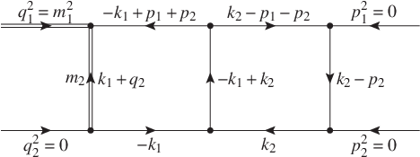
Fig. 1 shows a double box topology as it occurs for example in the NNLO QCD corrections to -channel single top-quark production [52, 53]. To start a reduction Kira requires certain configuration files specifying the topologies as well as kinematic relations. In addition, a job file describing the tasks to be performed by Kira is necessary.
In both cases the information is encoded in yaml files. Comments in yaml files are introduced using the # sign. yaml allows one to store lists and associative lists in an easy way. In the former case the list elements are either specified one in a line starting with - in so-called block format or in inline format encapsulated in square brackets []. Evidently, it is also possible to create lists of lists. In case of associative lists a colon is used to separate a key-value pair. An example of this notation may look like
momenta:
  - k1
  - k2
  - k3
loop_momenta: [l1, l2]
Note that yaml uses indentation for scoping, where only spaces but no tabs are allowed. The first 4 lines in the above example define momenta as a list of the three momenta k1,k2,k3 using the block format. Similar the fifth line declares loop_momenta as list of the two momenta l1,l2 using the inline format.
The double box diagram shown in Fig. 1 has loop momenta and independent external momenta. We use to denote the two loop momenta and and for the three external momenta. Momentum conservation is used to eliminate the fourth external momentum . In total we can thus form independent scalar products involving the loop momenta and . The scalar integral, which is associated with the Feynman diagram shown in Fig. 1, is given by
| (24) |
with
| (25) |
The propagators are associated with the internal lines, while the propagators and are auxiliary propagators. Kira uses the file integralfamilies.yaml located in the sub directory config of the working directory to provide the information about the topology. Note that this file can contain more than one topology which are distinguished by different names. For the example above, the file may look as follows.
#config/integralfamilies.yaml
integralfamilies:
  - name: "topo7"
    loop_momenta: [k1, k2]
    propagators:
      - ["-k1", 0]
      - ["k2", 0]
      - ["-k1+k2", 0]
      - ["k1+q2", m2^2]
      - ["k2-p2", 0]
      - ["-k1+p1+p2", 0]
      - ["k2-p1-p2", 0]
      - ["k1-p2", 0]
      - ["k2-q2", 0]
Since Kira can reduce several topologies in one run, the keyword name allows one to specify a name for each topology which can be used in other files to identify the topology and control the reduction to be done with Kira. The keyword loop_momenta is used to distinguish the loop momenta from the external momenta. The keyword propagators is followed by a list of the propagators. For each propagator the momentum flow and the mass is specified in the format ["l_i", m_iˆ2]. To provide information concerning kinematic relations like for example the masses of the external particles or the independent invariants which should be used to express the scalar products of external momenta, the yaml file kinematics.yaml is used. Like integralfamilies.yaml it must also be located in the subdirectory config. For the example shown in Fig. 1 the file may have the following form.
#config/kinematics.yaml
kinematics:
  incoming_momenta: [q1,q2,p1,p2]
  outgoing_momenta: []
  momentum_conservation: [q1,-p1-p2-q2]
  kinematic_invariants:
    - [s,  2]
    - [t,  2]
    - [m1, 1]
    - [m2, 1]
  scalarproduct_rules:
     - [[p1,p1],  0]
     - [[p2,p2],  0]
     - [[q2,q2],  0]
     - [[p1+p2, p1+p2], s]
     - [[p2-q2, p2-q2], t]
     - [[p1-q2, p1-q2], s-t-m1^2]
  symbol_to_replace_by_one: m1
The keywords incoming_momenta and outgoing_momenta are used to specify which external momenta are counted ingoing and which outgoing. Since in the above example we decided to count all momenta ingoing an empty list is provided for the outgoing momenta. The keyword momentum_conservation is used to specify which momentum can be removed by applying momentum conservation. Here, the momentum is replaced using
| (26) |
The variables which are used to denote the independent invariants are listed in the section introduced by the keyword kinematic_invariants. For each variable its name and its mass dimension is provided in a list with two elements. The section started with the keyword scalarproduct_rules expresses the scalar products of external momenta in terms of the invariants. To simplify the calculation it is very often useful—if not crucial—to reduce the number of independent mass scales by one by expressing all masses and scalar products in units of one freely chosen invariant. In these units the corresponding invariant is fixed to the numerical value one. The number of variables to be treated symbolically is thus reduced by one. To achieve this, the keyword symbol_to_replace_by_one is used. In the above example the mass is set to one.
As usual we assume that dimensional regularization is used to regulate divergent integrals. Kira uses the symbol d to specify the space time dimension. The symbol d is thus reserved and should not be used to describe momenta or invariants.
Having provided the information about the integral topology and the kinematics an additional yaml file is used to control Kira. The following lines show a minimal example:
#jobs1.yaml
jobs:
 - reduce_sectors:
    sector_selection:
      select_recursively:
        - [topo7,127]
    identities:
      ibp:
        - {r: [t,7], s: [0,1]}
Since the job file is provided as command line argument to Kira, the name can be freely chosen by the user. This file specifies how to prepare and run the reduction. In the first stage at runtime, the IBP and LI equations are derived in symbolic form and symmetry relations for the respective sectors are prepared. To calculate the IBP and LI equations in symbolic form Kira uses GiNaC [39, 40]. Also the trivial sectors are identified. In the second stage, the reduction is performed in four steps. First the system of equations is generated by evaluating the IBP and LI equations for specific powers (‘seeds’) of the propagators. In the next step, a linearly independent set of equations is chosen from the system of equations by the pyRed module. In the third step, the algorithm described in section 3.2.2 is applied to derive the upper-right triangular form. In the last step, the back substitution is performed as described in section 3.2.3. The individual steps of the reduction can be performed in separate runs.
To select the integral sectors to be reduced the keyword sector_selection is used followed by the method to select the sectors. At the moment only one method is available, namely
- select_recursively:
-
Select recursively all required sectors and sub-sectors to reduce the specified sector for a specific topology. Topology and sector are provided as a list of the form [topo, sector]. The sector is identified using the sector id as defined in Eq. (9). It is possible to provide more than one pair (topology, sector).
In the above example sector 127 of topology topo7 as specified in integralfamilies.yaml together with all required sub-sectors will be reduced.
In the setup phase Kira generates both the IBP as well as the LI relations in algebraic form. The keyword identities controls which seeds should be used to generate the system of equations. Note that in contrast to Reduze/Reduze 2 Kira always uses IBP and LI equations.
- ibp:
-
The allowed ranges for and as defined in Eq. (11). In the above example and are restricted to the range and . The variable is defined in Eq. (10). Kira replaces the symbol applying Eq. (10) to the current sector. If more than one associated list specifying the range for and is defined the set of seeds used in the run is the union.
Having prepared these files the working directory should contain the following files.
jobs1.yaml
config
config/integralfamilies.yaml
config/kinematics.yaml
To run the reduction Kira is started with the file name of the job file as command line argument,
kira jobs1.yaml
Note that to use Fermat, the path to the executable must be configured through the environment variable FERMATPATH, e.g. with
export FERMATPATH="/path/to/Fermat/fermat_executable"
After a successful run, Kira writes out the master integrals as identified during the reduction. In addition, for all topologies specified in the file integralfamilies.yaml the result of the reduction is stored topology wise in subdirectories of the directory results. The sector mappings and the trivial sectors of each topology are stored topology wise in subdirectories of the directory sectormappings. sectormappings and results are located in the working directory. In the above example only one topology is reduced and the directories results and sectormappings contain only one subdirectory topo7. The results directory contains for each topology the following files:
- id2int
-
The definition of the scalar integrals.
- kira
-
The result of the reduction.
- kira.db
-
An SQLite3 database storing the result of the reduction. The data can be inspected using the program SQLite3.
- masters
-
The potential master integrals as identified through the numerical reduction.
- masters.final
-
The potential master integrals as identified at the end of the reduction.
The sectormappings directory contains for each topology the following files:
- IBP
-
The IBP equations in symbolic form.
- LI
-
The LI equations in symbolic form.
- nonTrivialSector
-
The list of non-zero sectors. The second number counts the number of propagators.
- sectorRelations
-
Relations between sectors as determined by Kira.
- sectorSymmetries
-
Symmetries relating different integrals as determined by Kira
- topology_ordering
-
The order of the topologies as specified by the user.
- trivialsector
-
The list of zero sectors.
For the example discussed here, the result of the reduction for topo7 as stored in the file Kira may look:
- Eq:
  - [7697655529472,0,14,0,2,"1"]
  - [7696581394432,0,14,0,2,"(2*s+d-2)/d"]
- Eq:
  - [7697655791616,0,14,0,1,"1"]
- Eq:
  - [7697655267328,0,14,0,2,"1"]
  - [7696581394432,0,14,0,2,"((-d+2)*t)/d"]
...
Each equation is started with the keyword -Eq: and contains a list of integrals appearing in the equation. In the example only the first few lines of the output file are shown. The first entry of each list denotes the left hand side of the equation—the integral which is expressed in terms of the master integrals. The entries in the square bracket denote
- –
the ID of the integral,
- –
an integer specifying whether the integrals is a seed integral (0) or an auxiliary integral (-1)44 4 This field is mainly used for debugging. In the final result the entry should always be zero. ,
- –
the variable as defined in Eq. (9),
- –
the topology ,
- –
the length of the equation (=total number of integrals in the equation),
- –
and the algebraic coefficient of the corresponding integral.
To reduce the memory consumption during the run all integrals are mapped to an integer used to uniquely identify the integral. The definition of the integral ID’s is stored in the file results/topo7/id2int. The following lines show an example:
- [7696581394432,0,1,1,1,0,0,0,0,0,14,0,3,0,0,0]
- [7697655136256,-1,1,1,1,0,0,0,0,0,14,0,3,0,1,0]
- [7697655267328,0,1,1,1,-1,0,0,0,0,14,0,3,0,1,0]
- [7697655398400,0,1,1,1,0,-1,0,0,0,14,0,3,0,1,0]
- [7697655529472,0,1,1,1,0,0,-1,0,0,14,0,3,0,1,0]
...
The lines should be interpreted as follows:
[ID,,,,,,,,,,
,,,,,debug],
with , , , , as defined in section 2. Obviously, the
specification of , , , and is redundant since these
quantities can be calculated using the information for the .
Converted back to standard mathematical notation the first equation in the example shown above reads:
| (27) |
If an equation contains only one integral, the right hand side of the equation and thus the integral is zero. If a seed integral generated in the reduction does not appear in the output file this integral is also zero.
The following file illustrates an example in which specific tasks are to be performed.
#jobs2.yaml
jobs:
 - reduce_sectors:
    sector_selection:
      select_recursively:
        - [topo7,127]
    identities:
      ibp:
        - {r: [t,7],s: [0,1]}
    run_symmetries: true
    run_initiate: true
    run_pyred: true
    run_triangular: true
    run_back_substitution: true
Note that the two examples jobs1.yaml and jobs2.yaml perform the same tasks. The second example is given to illustrate how specific tasks can be started manually using options starting with run_. Starting individual tasks can also be used to resume a reduction stopped at an intermediate state.
- run_symmetries:
-
This option will only prepare the reduction. In particular, the IBP and LI equations are derived in symbolic form. Symmetry relations for the respective sector are prepared and trivial sectors are determined.
- run_initiate:
-
generate seeds in the allowed range and applies the IBP and the LI equations and the symmetry relations. The initiated system of equations is written to the files
tmp/[topo]/SYSTEM_[topo]_[sector_id].
The square brackets [topo] and [sector_id] are replaced by the topology name and the sector id, eg. tmp/topo7/SYSTEM_topo7_31. Implies run_symmetries. - run_pyred:
-
read the system of equations from the files
tmp/[topo]/SYSTEM_[topo]_[sector_id]
and run pyRed. The result is a list of integers stored in the file
tmp/[topo]/independentEQS.
Each integer references an equation in the files
tmp/[topo]/SYSTEM_[topo]_[sector_id].
The set of equations specifies the subset of linearly independent equations which will be solved in later steps. - run_triangular:
-
First the information stored in the file
tmp/[topo]/independentEQS
specifying the independent equations in files
tmp/[topo]/SYSTEM_[topo]_[sector_id]
is read, then the system of linearly independent equations is built. Having set up the system the algorithm to achieve the upper-right triangular form is started and the result is written to the files
tmp/[topo]/VER_[topo]_[sector_id]. - run_back_substitution:
-
Read the system of equations from the files
tmp/[topo]/VER_[topo]_[sector_id]
and run the algorithm for the back substitution. The result is a list of rules to express the seed integrals through the master integrals. These relations are written to the file
results/[topo]/kira.
Kira can reduce multiple integral families in the same run if they are listed in the job file jobs.yaml and are defined in the file integralfamilies.yaml. The following files illustrate this.
#config/integralfamilies.yaml
integralfamilies:
  - name: "topo7"
    loop_momenta: [k1,k2]
    top_level_sectors: [127]
    propagators:
      - ["-k1", 0]         #1
      - ["k2", 0]          #2
      - ["-k1+k2", 0]      #3
      - ["k1+q2", "m2^2"]  #4
      - ["k2-p2", 0]       #5
      - ["-k1+p1+p2", 0]   #6
      - ["k2-p1-p2", 0]    #7
      - ["k1-p2", 0]       #8
      - ["k2-q2", 0]       #9
  - name: "topo7x"
    loop_momenta: [k1,k2]
    top_level_sectors: [508]
    propagators:
      - ["k1-p2", 0]       #8
      - ["k2-q2", 0]       #9
      - ["-k1", 0]         #1
      - ["k2", 0]          #2
      - ["k1+q2", "m2^2"]  #4
      - ["k2-p2", 0]       #5
      - ["-k1+k2", 0]      #3
      - ["k2-p1-p2", 0]    #7
      - ["-k1+p1+p2", 0]   #6
Obviously, the two topologies differ only by the order of the propagators. This example illustrates that Kira is able to map sub-sectors of different topologies on each other and determines a common set of master integrals for the different integral families considered in one run. Running the reduction for the two topologies separately one will end up with different master integrals which would need to be mapped on each other in a separate run. The following example shows the job file to reduce both topologies (topo7 and topo7x) in one run.
Symmetries are identified topology wise and integrals are preferably mapped to topologies which have been defined earlier and to sectors with lower ID. One may restrict symmetries such that integrals are only mapped to sub-sectors of user-defined top-level sectors of each topology using the following option in integralfamilies.yaml.
- top_level_sectors: []
-
One may define multiple sectors for each topology, is defined in equation (9).
The following example illustrates a couple of advanced features to tune the reduction.
#jobs3.yaml
jobs:
 - reduce_sectors:
    sector_selection:
      select_recursively:
       - [topo7, 127]
       - [topo7x, 508]
    identities:
     ibp:
        - {r: [t,7], s: [0,2]}
        - {r: [t,8], s: [0,1]}
    select_integrals:
      select_mandatory_recursively:
       - [topo7, 127, 1, 2]
       - [topo7x, 508, 1, 2]
      select_mandatory_list:
       - [topo7, seeds7]
       - [topo7x, seeds7x]
    run_initiate: true
    run_pyred: true
    run_triangular: true
    run_back_substitution: true
    conditional: true
    alt_dir: "/path/to/alternative_dir"
Instead of using all linearly independent equations generated from the seeds within the specified boundaries one can let pyRed choose a smaller system which is sufficient to reduce a user-provided list of integrals. This is turned on with the keyword select_integrals followed by the options:
- select_mandatory_recursively: [[topo,,,]]
-
For the topology topo (specified via the file integralfamilies.yaml) choose a set of equations which is sufficient to reduce the seed integrals bounded by (,,). , , , are defined in section 2. The unreduced integrals, which are regarded as the master integrals are written to the file results/[topo]/masters.
- select_mandatory_list: [[topo,file]]
-
Choose a set of equations which is sufficient to reduce the integrals specified in the file file for topology topo. The unreduced integrals, which are regarded as the master integrals are written to the file
results/[topo]/masters.
Note, that Kira does not guarantee that all integrals within a rectangular seed selection can be reduced. When the option select_mandatory_recursively is invoked, Kira will print the master integrals after the numerical reduction. If an integral at the edge of the seed range appears as a master integral, this integral is unreduced. In this case the user needs to enlarge the rectangular seed selection and restart Kira.
The option alt_dir can be used to specify a directory for the intermediate and final results.
- alt_dir: "/path/to/alternative_dir"
-
All temporary and result files will be saved and loaded from the directories
"/path/to/alt_dir/tmp", "/path/to/alt_dir/results" and
"/path/to/alt_dir/sectormappings". If alt_dir is not specified, the working directory is used.
- conditional: true
-
In Kira the results of a backward substitution will be commited to the database kira.db every 10 minutes. Since Kira version 1.1 the backward substitution can be killed at any time. To resume the backward substitution and to load the results from a previous run the option conditional must be set to true. An option to interrupt the backward substitution gracefully will be provided in a future Kira version.
As mentioned before, each equation in the result file Kira represents a rule to replace a seed integral through the master integrals. To extract the results in a specific format usable in computer algebra programs like FORM [54] or Mathematica one may use the following options in the job file.
- - kira2form:
-
With target: [[topo,seeds]] the integrals of topology topo listed in the file seeds will be translated into a FORM readable file:
results/topo/kira_seeds.inc.
With target: [[topo,,,]] it is possible to reconstruct all integrals for the topology topo (specified via the file integralfamilies.yaml), which are bounded by (,,). , , , are defined in section 2. The result will be written into a FORM readable file: results/topo/kira___.inc.
If during the reduction the option alt_dir: "/path/..." was used, then the option alt_dir: "/path/..." is mandatory. Kira will look for the results of the reduction in the directory specified via the option alt_dir. - - kira2math:
-
This option is similar to the option - kira2form:. Here the results will be written into Mathematica readable files ending with .m
By default, the dependence of coefficients in the symbol which was replaced by one during the reduction with the option symbol_to_replace_by_one will not be reconstructed. This can be activated with the option reconstruct_mass: true. An example of a file containing the seed integrals is shown here.
#seeds7
- [0,1,1,1,-1,0,0,0,0]
- [0,1,1,1,0,0,-1,0,0]
- [1,1,1,1,1,0,0,0,0]
- [1,1,1,1,2,0,0,0,0]
A job file extracting various identities in FORM and Mathematica readable form may look like
#export.yaml
jobs:
 - kira2math:
   target:
     - [topo7x,seeds7x]
     - [topo7,seeds7]
     - [topo7,127,1,2]
   reconstruct_mass: true
 - kira2form:
   target:
     - [topo7x,seeds7x]
     - [topo7,seeds7]
In case the option kira2form is used the file kira_seeds7.inc contains identities of the form
id topo7(0,1,1,1,-1,0,0,0,0) =
 + topo7(0,1,1,1,0,0,0,0,0)*(((-d+2)*t)*den(d))
;

id topo7(0,1,1,1,0,0,-1,0,0) =
 + topo7(0,1,1,1,0,0,0,0,0)*((2*s+d-2)*den(d))
;
...
In case kira2math is used the file kira_seeds7.m looks like
{
topo7[0,1,1,1,-1,0,0,0,0] ->
 + topo7[0,1,1,1,0,0,0,0,0]*(((-d+2)*t)/d)
,
topo7[0,1,1,1,0,0,-1,0,0] ->
 + topo7[0,1,1,1,0,0,0,0,0]*(((d-2)*m1^2+2*s)/d)
,
...}
The Mathematica readable format can be included in Mathematica using the command
rule = Get["results/topo7/kira_seeds7.m"];
For the above example a Mathematica session may look like this
In[1]:= rule = Get["results/topo7/kira_seeds7.m"];

In[2]:= topo7[0,1,1,1,0,0,-1,0,0] /. rule

                    2
        ((-2 + d) m1  + 2 s) topo7[0, 1, 1, 1, 0, 0, 0, 0, 0]
Out[2]= -----------------------------------------------------
                                  d
In this example the mass was reconstructed.
In addition to the options which can be specified in the configuration files the following command line arguments are recognized by Kira.
- --version
-
Print out the current Kira version.
- --help
-
Print out a brief description of the command line arguments and how to use Kira.
- --silent
-
Suppresses the output to the screen during the run. Note that the log file kira.log is still written.
- --parallel=n
-
Run instances of Fermat in parallel. During the back substitution significant runtime is spent for the algebraic simplification of the integral coefficients. Performing this step in parallel can lead to a significant speed-up. In the current Kira version the maximal number of parallel tasks is unlimited. The value set by the user should not exceed the number of processor cores available. Also the generation of the IBP and LI equations and the algorithm to build the upper-right triangular form are run in parallel.
- --algebra
-
For multi-scale problems the integral coefficients tend to become rather large. In this case the option --algebra might be useful. This enables a modified algorithm for the back substitution and in particular the sorting algorithm described in section 3.2.3.
The following Reduze 2 options are supported in Kira:
jobs:
  - reduce_sectors:
    sector_selection:
      select_recursively:
    identities:
      ibp:
integralfamilies:
  - name:
    loop_momenta:
    propagators:
    cut_propagators:
kinematics:
  incoming_momenta:
  outgoing_momenta:
  momentum_conservation:
  kinematic_invariants:
  scalarproduct_rules:
  symbol_to_replace_by_one:
6 Benchmarks


To benchmark the performance of our implementation we study three examples, occurring in the evaluation of NNLO corrections to -channel single top-quark production. The first example is the planar double box topo7 shown in Fig. 1. The second example is a non planar topology topo4 shown in Fig. 2. The integral associated with topo4 is given by Eq. (24), with the following definition of the propagators:
The third example is the non planar topology topo5 shown in Fig. 3. This turns out to be the most complicated topology in single top-quark production at NNLO. The integral associated with topo5 is again given by Eq. (24), with the following propagators,
In both cases the propagators are associated with the internal lines, while the propagators and are auxiliary propagators.
| Type | ||||||||
| default | 1 | 1.1 s | 142 s | 2 h | 17 min | 0.008 | 51 | 7.1 |
| A | 1 | 2.6 s | 49.5 s | - | 6.7 min | 0.053 | - | 8.1 |
| B | 1 | 2.6 s | 40 s | - | 1 s | 0.065 | - | 0.025 |
| default | 2 | 4.5 s | 664 s | 10 h | 87 min | 0.007 | 54 | 7.9 |
| A | 2 | 4.5 s | 224 s | - | 20.3 min | 0.02 | - | 5.4 |
| B | 2 | 4.5 s | 203 s | - | 17.6 min | 0.022 | - | 5.2 |
| default | 3 | 11 s | 48.5 min | 28.4 h | 4.7 h | 0.0004 | 35 | 5.8 |
| A | 3 | 11 s | 14.2 min | - | 1.47 h | 0.013 | - | 6.2 |
| B | 3 | 11 s | 10.7 min | - | 1.3 h | 0.017 | - | 7.3 |
| default | 4 | 23 s | 4.1 h | 4.4 d | 13.6 h | 0.0015 | 25 | 3.3 |
| A | 4 | 23 s | 1.2 h | - | 4.5 h | 0.005 | - | 3.75 |
| B | 4 | 23 s | 35.4 min | - | 3.9 h | 0.01 | - | 6.6 |
All benchmarks were run on compute nodes equipped with two Intel(R) Xeon(R) E5-2680 CPUs (8 cores/CPU) clocked at 2.70 GHz and 396 GBytes of RAM.
As described in the previous section, Kira offers the ability to reduce only selected integrals using the option select_integrals. We study three different types of jobs to reduce integrals of the complexity . The jobs of type default do not employ the option select_integrals. Type A jobs use the option select_mandatory_recursively: [[topo,127,0,]], where topo is replaced by topo4 or topo7. This option forces Kira to reduce integrals with (zero dots) and . Finally, the jobs of type B use the option select_mandatory_list: [[topo,list]], where topo is again replaced by topo4 and topo7 and list is replaced by list1, list2, list3 and list4 for , respectively:
#list1
- [1,1,1,1,1,1,1, 0,-1]
- [1,1,1,1,1,1,1,-1, 0]

#list2
- [1,1,1,1,1,1,1, 0,-2]
- [1,1,1,1,1,1,1,-2, 0]
- [1,1,1,1,1,1,1,-1,-1]

#list3
- [1,1,1,1,1,1,1, 0,-3]
- [1,1,1,1,1,1,1,-3, 0]
- [1,1,1,1,1,1,1,-2,-1]
- [1,1,1,1,1,1,1,-1,-2]

#list4
- [1,1,1,1,1,1,1, 0,-4]
- [1,1,1,1,1,1,1,-4, 0]
- [1,1,1,1,1,1,1,-1,-3]
- [1,1,1,1,1,1,1,-3,-1]
- [1,1,1,1,1,1,1,-2,-2]
We start our discussion with the reduction of topology topo7. In the benchmark we use the parameter , counting the total power of propagators in the numerator, to control the complexity of the reduction. For all reductions we have checked that Kira, Reduze 2 and FIRE 555 5 The used Fermat is 64 bit Linux version 5.25. For the benchmarks with Reduze 2 we used version 2.1.2 (MPI build) and with FIRE 5 we used version 5.2. produce the same set of master integrals and that the results for the reduced integrals agree. Tab. 1 shows the runtime used by Kira and Reduze 2. In addition, we report also the runtime used by the pyRed module. While the time used in pyRed is small compared to the total runtime, removing the linearly dependent equations significantly reduces the total time required by Kira. We observe that in the considered examples Kira is between 1–2 orders of magnitude faster than Reduze 2. For the reduction of type default Kira is up to 1 order of magnitude faster than FIRE 5, but for the reduction type A and type B Kira is between 1–2 orders of magnitude faster than FIRE 5.
| Type | ||||||||
| default | 1 | 2.8 s | 90 s | 2.1 h | 23 min | 0.03 | 86 | 15.3 |
| A | 1 | 2.8 s | 23.6 s | - | 19.3 min | 0.11 | - | 49 |
| B | 1 | 2.8 s | 16.1 s | - | 1.6 s | 0.17 | - | 0.1 |
| default | 2 | 9.8 s | 6.6 min | 7.2 h | 2.3 h | 0.02 | 65 | 21 |
| A | 2 | 11.3 s | 167 s | - | 2.2 h | 0.07 | - | 47 |
| B | 2 | 11.2 s | 160 s | - | 2.2 h | 0.07 | - | 50 |
| default | 3 | 28 s | 43 min | 22.8 h | 7.6 h | 0.01 | 32 | 10.6 |
| A | 3 | 30.4 s | 539 s | - | 7.4 h | 0.06 | - | 49.4 |
| B | 3 | 30.1 s | 444 s | - | 7.5 h | 0.07 | - | 61 |
| default | 4 | 67 s | 2.4 h | 2.7 d | 23.5 h | 0.007 | 26 | 9.8 |
| A | 4 | 70.2 s | 35.3 min | - | 22.4 h | 0.03 | - | 38 |
| B | 4 | 69.5 s | 24 min | - | 22.4 h | 0.05 | - | 56 |
In case of topology topo4 the additional mass scale leads to a significant increase in complexity. In single top-quark production corresponds to the top-quark mass and is the boson mass. In Ref. [52] a fixed ratio between the two masses was used to reduce the number of independent scales and thus the complexity of the reduction. In the benchmark presented here we follow the same strategy and set
| (28) |
The runtime required for the reduction of the topology topo4 is given in Tab. 2. Since in the pyRed module the invariants are replaced by integer values the runtime for this part of the reduction is similar to the runtime observed for the topology topo7. Again only a small fraction of the total runtime is required to identify the linearly dependent equations. Even for the most complicated reduction the required runtime is roughly a minute. Reduze 2, FIRE 5 as well as Kira were all started with 11 cores allowing to perform a significant part of the reduction in parallel. The examples presented in Tab. 1 and Tab. 2 require very little memory. An amount of 4 GBytes is sufficient to run the examples. In Tabs. 1 and 2 we observe that the jobs of type A and type B improve the runtime of Kira by a factor of 3–5 compared to the job of type default without selecting the integrals with the option select_integrals.
| topo4 | 8 | 3 | 41 s | 14 h | 0.0008 |
| 7 | 4 | 130 s | 10 h | 0.003 | |
| topo5 | 8 | 2 | 94 s | 3 d | 0.0003 |
| 8 | 3 | 125 s | 8 d | 0.0002 | |
| 7 | 4 | 237 s | 7 d | 0.0004 |
As a final benchmark we study the reduction of topo4 and topo5 keeping the full mass dependence. The runtime required is shown in Tab. 3. The reduction was done using 13 processor cores. In addition, the command line option --algebra was used to reduce the time required for the back substitution. Comparing the results for topology topo4 shown in Tab. 2 and Tab. 3, we observe that the additional mass scale leads to significant increase in the total runtime. As mentioned before, the time required by the pyRed module to eliminate the linearly dependent equations is only mildly affected since this part is based on integer arithmetic. For topo4 the total runtime is of the order of 10 hours while for topo5 the most challenging reductions take roughly one week. Most of the time is spent on the algebraic simplifications of the integral coefficients using Fermat. This is also reflected in significantly increased memory consumption. To reproduce the results shown in Tab. 3 about 90 GBytes of RAM is required in Kira plus around 10 GBytes for each Fermat instance. Again, for all reductions we have checked that Kira and Reduze 2 produce the same set of master integrals. To compare the reduction against Reduze 2 we ran Reduze 2 with numerical input values for the kinematics instead of symbolic input.
The gain in performance using the option --algebra is illustrated in Tab. 4. As expected the improvement depends on the complexity. For the simplest case () the total runtime is roughly reduced by a factor 2. Increasing the complexity () a total speed-up by roughly a factor 4.5 is achieved.
| options | |||
|---|---|---|---|
| 1 | 495 s | 543 s | --algebra --parallel=16 |
| 1 | 1108 s | 1156 s | --parallel=16 |
| 2 | 2920 s | 3354 s | --algebra --parallel=16 |
| 2 | 6683 s | 7096 s | --parallel=16 |
| 3 | 13203 s | 13664 s | --algebra --parallel=16 |
| 3 | 59905 s | 60370 s | --parallel=16 |
7 Conclusion
In this article we presented a new implementation of the Laporta algorithm to reduce multi-loop Feynman integrals to a small set of master integrals. Compared to previous implementations an algorithm based on modular arithmetic is used to eliminate linearly dependent equations from the set of IBP and LI relations. Using only the linearly independent equations the system is brought into upper triangle form using a straight forward Gauss elimination. For the backward substitution an optimized procedure delaying the expression swell of intermediate expressions has been implemented. Removing linearly dependent equations in combination with the optimized back substitution leads to a significant increase in performance when complicated topologies are reduced. Particularly multi-scale problems benefit from these improvements. To illustrate the mentioned features we have successfully reproduced various reductions occurring in the calculation of the NNLO corrections to single top-quark production. We also stress that the algorithm is not limited to two-loop corrections but can be applied also to higher loop reductions.
Acknowledgments:
J.U. would like to thank Bas Tausk for his very useful discussions during the early stage of this project. We wish to express our special thanks to Andreas von Manteuffel, Tord Riemann and Bas Tausk for a careful reading of the manuscript and useful comments. The work of J.U. is supported by the research training group GRK-1504 “Masse, Spektrum, Symmetrie” funded by the German research foundation (DFG) and received funding from the European Research Council (ERC) under the European Union’s Horizon 2020 research and innovation programme under grant agreement no. 647356 (CutLoops). P.M. acknowledges support by the state of Baden-Württemberg through bwHPC and the German Research Foundation (DFG) through grant no INST 39/963-1 FUGG.
References
- [1] M. Czakon, P. Fiedler, and A. Mitov, Total Top-Quark Pair-Production Cross Section at Hadron Colliders Through , Phys. Rev. Lett. 110 (2013) 252004, arXiv:1303.6254 [hep-ph].
- [2] R. Boughezal, F. Caola, K. Melnikov, F. Petriello, and M. Schulze, Higgs boson production in association with a jet at next-to-next-to-leading order, Phys. Rev. Lett. 115 no. 8, (2015) 082003, arXiv:1504.07922 [hep-ph].
- [3] X. Chen, T. Gehrmann, E. W. N. Glover, and M. Jaquier, Precise QCD predictions for the production of Higgs + jet final states, Phys. Lett. B740 (2015) 147–150, arXiv:1408.5325 [hep-ph].
- [4] J. M. Lindert, K. Melnikov, L. Tancredi, and C. Wever, Top-bottom interference effects in Higgs plus jet production at the LHC, arXiv:1703.03886 [hep-ph].
- [5] S. Borowka, N. Greiner, G. Heinrich, S. Jones, M. Kerner, J. Schlenk, U. Schubert, and T. Zirke, Higgs Boson Pair Production in Gluon Fusion at Next-to-Leading Order with Full Top-Quark Mass Dependence, Phys. Rev. Lett. 117 no. 1, (2016) 012001, arXiv:1604.06447 [hep-ph]. [Erratum: Phys. Rev. Lett.117,no.7,079901(2016)].
- [6] A. Gehrmann-De Ridder, T. Gehrmann, E. W. N. Glover, A. Huss, and T. A. Morgan, Precise QCD predictions for the production of a Z boson in association with a hadronic jet, Phys. Rev. Lett. 117 no. 2, (2016) 022001, arXiv:1507.02850 [hep-ph].
- [7] R. Boughezal, J. M. Campbell, R. K. Ellis, C. Focke, W. T. Giele, X. Liu, and F. Petriello, Z-boson production in association with a jet at next-to-next-to-leading order in perturbative QCD, Phys. Rev. Lett. 116 no. 15, (2016) 152001, arXiv:1512.01291 [hep-ph].
- [8] R. Boughezal, C. Focke, X. Liu, and F. Petriello, -boson production in association with a jet at next-to-next-to-leading order in perturbative QCD, Phys. Rev. Lett. 115 no. 6, (2015) 062002, arXiv:1504.02131 [hep-ph].
- [9] M. Grazzini, S. Kallweit, D. Rathlev, and M. Wiesemann, production at hadron colliders in NNLO QCD, Phys. Lett. B761 (2016) 179–183, arXiv:1604.08576 [hep-ph].
- [10] M. Grazzini, S. Kallweit, and D. Rathlev, and production at the LHC in NNLO QCD, JHEP 07 (2015) 085, arXiv:1504.01330 [hep-ph].
- [11] T. Gehrmann, M. Grazzini, S. Kallweit, P. Maierhöfer, A. von Manteuffel, S. Pozzorini, D. Rathlev, and L. Tancredi, Production at Hadron Colliders in Next to Next to Leading Order QCD, Phys. Rev. Lett. 113 no. 21, (2014) 212001, arXiv:1408.5243 [hep-ph].
- [12] F. Caola, K. Melnikov, R. Röntsch, and L. Tancredi, QCD corrections to production through gluon fusion, Phys. Lett. B754 (2016) 275–280, arXiv:1511.08617 [hep-ph].
- [13] F. Caola, J. M. Henn, K. Melnikov, A. V. Smirnov, and V. A. Smirnov, Two-loop helicity amplitudes for the production of two off-shell electroweak bosons in gluon fusion, JHEP 06 (2015) 129, arXiv:1503.08759 [hep-ph].
- [14] F. Cascioli, T. Gehrmann, M. Grazzini, S. Kallweit, P. Maierhöfer, A. von Manteuffel, S. Pozzorini, D. Rathlev, L. Tancredi, and E. Weihs, ZZ production at hadron colliders in NNLO QCD, Phys. Lett. B735 (2014) 311–313, arXiv:1405.2219 [hep-ph].
- [15] F. Caola, K. Melnikov, R. Röntsch, and L. Tancredi, QCD corrections to ZZ production in gluon fusion at the LHC, Phys. Rev. D92 no. 9, (2015) 094028, arXiv:1509.06734 [hep-ph].
- [16] J. Currie, T. Gehrmann, A. Huss, and J. Niehues, NNLO QCD corrections to jet production in deep inelastic scattering, arXiv:1703.05977 [hep-ph].
- [17] C. Anastasiou, C. Duhr, F. Dulat, E. Furlan, T. Gehrmann, F. Herzog, A. Lazopoulos, and B. Mistlberger, High precision determination of the gluon fusion Higgs boson cross-section at the LHC, JHEP 05 (2016) 058, arXiv:1602.00695 [hep-ph].
- [18] I. Dubovyk, A. Freitas, J. Gluza, T. Riemann, and J. Usovitsch, The two-loop electroweak bosonic corrections to , Phys. Lett. B762 (2016) 184–189, arXiv:1607.08375 [hep-ph].
- [19] I. Dubovyk, J. Gluza, T. Riemann, and J. Usovitsch, Numerical integration of massive two-loop Mellin-Barnes integrals in Minkowskian regions, PoS LL2016 (2016) 034, arXiv:1607.07538 [hep-ph].
- [20] I. Dubovyk, A. Freitas, J. Gluza, T. Riemann, and J. Usovitsch, 30 years, some 700 integrals, and 1 dessert, or: Electroweak two-loop corrections to the Zb vertex, PoS LL2016 (2016) 075, arXiv:1610.07059 [hep-ph].
- [21] F. V. Tkachov, A Theorem on Analytical Calculability of Four Loop Renormalization Group Functions, Phys. Lett. B100 (1981) 65–68.
- [22] K. G. Chetyrkin and F. V. Tkachov, Integration by Parts: The Algorithm to Calculate beta Functions in 4 Loops, Nucl. Phys. B192 (1981) 159–204.
- [23] T. Gehrmann and E. Remiddi, Differential equations for two loop four point functions, Nucl. Phys. B580 (2000) 485–518, arXiv:hep-ph/9912329 [hep-ph].
- [24] S. Laporta, High precision calculation of multiloop Feynman integrals by difference equations, Int.J.Mod.Phys. A15 (2000) 5087–5159, arXiv:hep-ph/0102033 [hep-ph].
- [25] C. Anastasiou and A. Lazopoulos, Automatic integral reduction for higher order perturbative calculations, JHEP 07 (2004) 046, arXiv:hep-ph/0404258 [hep-ph].
- [26] A. V. Smirnov, Algorithm FIRE – Feynman Integral REduction, JHEP 10 (2008) 107, arXiv:0807.3243 [hep-ph].
- [27] A. V. Smirnov and V. A. Smirnov, FIRE4, LiteRed and accompanying tools to solve integration by parts relations, Comput. Phys. Commun. 184 (2013) 2820–2827, arXiv:1302.5885 [hep-ph].
- [28] A. V. Smirnov, FIRE5: a C++ implementation of Feynman Integral REduction, Comput. Phys. Commun. 189, 182 (2015), arXiv:1408.2372 [hep-ph]].
- [29] C. Studerus, Reduze-Feynman Integral Reduction in C++, Comput. Phys. Commun. 181 (2010) 1293–1300, arXiv:0912.2546 [physics.comp-ph].
- [30] A. von Manteuffel and C. Studerus, Reduze 2 - Distributed Feynman Integral Reduction, arXiv:1201.4330 [hep-ph].
- [31] P. Kant, Finding Linear Dependencies in Integration-By-Parts Equations: A Monte Carlo Approach, Comput. Phys. Commun. 185 (2014) 1473–1476, arXiv:1309.7287 [hep-ph].
- [32] R. N. Lee and A. A. Pomeransky, Critical points and number of master integrals, JHEP 11 (2013) 165, arXiv:1308.6676 [hep-ph].
- [33] A. Georgoudis, K. J. Larsen, and Y. Zhang, Azurite: An algebraic geometry based package for finding bases of loop integrals, arXiv:1612.04252 [hep-th].
- [34] R. N. Lee, LiteRed 1.4: a powerful tool for reduction of multiloop integrals, J. Phys. Conf. Ser. 523 (2014) 012059, arXiv:1310.1145 [hep-ph].
- [35] B. Ruijl, T. Ueda, and J. A. M. Vermaseren, Forcer, a FORM program for the parametric reduction of four-loop massless propagator diagrams, arXiv:1704.06650 [hep-ph].
- [36] H. Ita, Two-loop Integrand Decomposition into Master Integrals and Surface Terms, Phys. Rev. D94 no. 11, (2016) 116015, arXiv:1510.05626 [hep-th].
- [37] K. J. Larsen and Y. Zhang, Integration-by-parts reductions from unitarity cuts and algebraic geometry, Phys. Rev. D93 no. 4, (2016) 041701, arXiv:1511.01071 [hep-th].
- [38] R. N. Lee, Presenting LiteRed: a tool for the Loop InTEgrals REDuction, arXiv:1212.2685 [hep-ph].
- [39] C. W. Bauer, A. Frink, and R. Kreckel, Introduction to the GiNaC framework for symbolic computation within the C++ programming language, J. Symb. Comput. 33 (2000) 1, arXiv:cs/0004015 [cs-sc].
- [40] J. Vollinga, GiNaC: Symbolic computation with C++, Nucl. Instrum. Meth. A559 (2006) 282–284, arXiv:hep-ph/0510057 [hep-ph].
- [41] M. Kauers, Fast solvers for dense linear systems, Nucl. Phys. Proc. Suppl. 183 (2008) 245–250.
- [42] A. von Manteuffel and R. M. Schabinger, A novel approach to integration by parts reduction, Phys. Lett. B744 (2015) 101–104, arXiv:1406.4513 [hep-ph].
- [43] J. von zur Gathen, and J. Gerhard, Modern Computer Algebra (3rd ed.), Cambridge University Press, (2013).
- [44] T. Peraro, Scattering amplitudes over finite fields and multivariate functional reconstruction, JHEP 12 (2016) 030, arXiv:1608.01902 [hep-ph].
- [45] A. von Manteuffel and R. M. Schabinger, Quark and gluon form factors to four-loop order in QCD: the contributions, Phys. Rev. D95 no. 3, (2017) 034030, arXiv:1611.00795 [hep-ph].
- [46] R. H. Lewis, Computer Algebra System Fermat. http://www.bway.net/lewis.
- [47] M. Tentioukov, gateToFermat. http://science.sander.su/FLink.htm.
- [48] SQLite, SQLite3, version: 3.14.2. https://www.sqlite.org.
- [49] B. Haible and R. B. Kreckel, CLN - Class Library for Numbers, version 1.3.4. http://www.ginac.de/CLN.
- [50] YAML, YAML Ain’t Markup Language. http://yaml.org.
- [51] J.-L. Gailly and M. Adler, ZLIB. http://zlib.net.
- [52] M. Assadsolimani, P. Kant, B. Tausk, and P. Uwer, Calculation of two-loop QCD corrections for hadronic single top-quark production in the channel, Phys. Rev. D90 no. 11, (2014) 114024, arXiv:1409.3654 [hep-ph].
- [53] M. Brucherseifer, F. Caola, and K. Melnikov, On the NNLO QCD corrections to single-top production at the LHC, Phys. Lett. B736 (2014) 58–63, arXiv:1404.7116 [hep-ph].
- [54] J. A. M. Vermaseren, New features of FORM, arXiv:math-ph/0010025 [math-ph].