Supersymmetric hybrid inflation with non-minimal coupling to gravity
Abstract
We have studied the paradigm of cosmic inflation using the simplest model based on the idea of supersymmetric hybrid inflation with non-minimal coupling to gravity, specially under the slow-roll approximation following the superconformal approach to supergravity. It is found that within a range of values of the non-minimal coupling parameter , the model can accommodate the inflation data reported by the Planck ( and upper limit of ) and BICEP2/Keck (upper limit of ) collaborations. The study shows that the most probable value of should be . That is coupling is found to be very week. Within this range of , the values of estimated from our model for e-foldings are found to be laying well below the upper limits set by the Planck and BICEP2/Keck collaborations. Similarly, values of obtained for the said parameters are in good agreement with its latest data of the Planck collaboration. The constraint equations for the running of the scalar spectral index and its running are derived from the numerical solutions of our model for these parameters. These equations can be used to test our model from the data of future cosmological observations.
Keywords
Supersymmetry, Cosmology, Inflation1 Introduction
The paradigm of cosmic inflation [1, 2, 3, 4, 5, 6, 7] not only solved the outstanding problems of modern cosmology, such as the horizon and flatness problems [6, 7], but also it explains the origin of the temperature anisotropy of Cosmic Microwave Background (CMB) radiation as observed by the Cosmic Background Explorer (COBE) satellite [8]. The recent observations of the Planck satellite [9, 10] on the CMB anisotropies has provided even more strong evidence of the existence of the epoch of inflation. The tempting evidence of the cosmic inflation comes from the BICEP2 experiment [11], who recently claimed to has been detected the B-mode polarization of the CMB temperature anisotropy. These detected B-modes are supposed to be generated by primordial gravitational waves, which are due to quantum fluctuations of the graviton. So, if this result is confirmed by future checks then it will establish that the gravity is ultimately a quantum theory. This would imply that the physics of cosmic inflation, which we still do not understand in the fully fundamental sense, lies beyond the standard model. However, the latest results from the analysis of data taken by the BICEP2 and Keck Array [12] set a (combined) upper limit for the B-mode polarization that is in consistent with the upper limit set by the most recent results of Planck experiment [10] as well as set by the WMAP experiment [13] earlier.
According to a large number of models of cosmic inflation, the inflation is generated by a homogeneous scalar field, called inflaton, which under suitable conditions may lead to an early-time accelerated expansion of the Universe. The magnitude of the inflaton field is typically very large at the beginning of the inflation and then it rolls down towards a potential minimum where the inflation ends (as an example for chaotic inflation see Ref. [14]). Another important but complex class of models which are based on a phase transition between two scalar fields are known as hybrid or double inflation models [15, 16]. In the hybrid inflation scenario one of the two interacting fields generates the inflation and is known as the inflaton field as usual. The second field which is dubbed as the waterfall field remains ineffective during inflation, but it ends the inflation by triggering an instability at a time when the inflaton field reaches the minimum of its potential. The waterfall field is a heavy field so that it can generate sufficient instability to stop the inflation.
As the inflation takes place at a much higher energy scale (the Planck scale) than the electroweak energy scale, a hierarchy problem exists between these two energy scales [17]. One of the most effective natural solution to this problem is the implementation of the theory of supersymmetry (SUSY) [18], which ensures the stability of such a large hierarchy against radiative corrections, to the theory of inflation. This stability is very essential to keep the flatness of inflaton potential at the quantum level. Thus, it is important to study inflation in the framework of the gravity version of SUSY, i.e., in the framework of supergravity. The hybrid inflation scenario has the natural structure that is suitable to incorporate the framework of supergravity within it. The only new constraint brought to this scenario by supergravity is that, the inflaton field values should be less than the reduced Planck mass, otherwise flatness of the potential may be destroyed making the onset of inflation more difficult [19, 20].
Application of SUSY to the inflationary paradigm shows that the Higgs doublet superfield has to play the role of inflaton field. This supersymmertic Higgs model inflation requires only local SUSY, i.e. supergravity to solve the Einstein equation. Again for the mass of the Higgs field to lie within the bound set by current findings of LHC [21] and to get sufficiently flat Higgs field potential, there must be a large non-minimal coupling of the Higgs field to the curvature scalar, of the form . The Jordan frame action of the inflaton field in such models contain a canonical kinetic term of the Higgs field but the gravity part of the action changes due to the non-minimal coupling of gravity with Higgs field. With this action it is not possible to use familiar equation of general relativity, the inflationary solutions and the standard slow-roll analysis. However, all these can be achieved if one makes the transformation of the action from Jordan frame to the Einstein frame where variables show minimal coupling between the Higgs field and the gravity [22]. This transformation can be done by the superconformal approach to supergravity developed in [23], so that the original superconformal symmetry can be recovered. Most recently there is a wave of interest to implement the supergravity in the inflationary paradigm using non-minimal gravity coupling with the Higgs inflation field via superconformal approach to supergravity (e.g. see [17, 24, 25, 26, 27, 28, 29, 30, 31, 32, 33, 34, 35, 36, 37, 38, 39, 40, 41, 42, 43, 44, 45] and references therein). This wave is mainly to study the behaviour of various models derived in the past in the context of general relativity coupled to scalar fields with or without supersymmetry. The flow in this context is mainly concentrated towards the direction of the chaotic inflation scenario only. However, in Refs.[46, 47, 48, 49, 50] different aspects of inflation including primordial perturbations and isocurvature modes were studied using the multifield model with non-minimal coupling to gravity within the domain of standard theories. Similarly, the connection between hybrid inflation and the models of Higgs inflation in supergravity with non-minimal coupling was analysed in the Refs.[51, 52], wherein it was shown that the observable gravitational waves can be achieved by avoiding transplanckian excursions of the initial (non-canonically normalized) inflaton and without provoking any problem with perturbative unitarity. Thus study of hybrid inflationary models in supergravity with non-minimal coupling to gravity would be interesting and hence it invites our attention in this direction.
There are two types of hybrid inflation models derived from SUSY: F-term and D-term hybrid inflation [53]. As the F-term type naturally fits with the Higgs mechanism so most of the studies are done on this type of hybrid inflation models only. As such, in this work we study the simplest F-term SUSY hybrid inflation model [54, 55] with a non-minimal coupling to gravity to see the consequences of this coupling in a simplest possible mean. In this context, it should be mentioned that in the Ref.[56] a systematic study was done on the suitability of inflation model building in Jordan frame supergravity, where it shows that the inflationary models have strong dependency on non-minimal coupling to gravity and in many cases the supergravity contributes to the flattening of the potential in the Einstein frame, that would be suitable for slow-roll inflation. Here, we will basically investigate the above cited model in the Einstein frame under the slow-roll inflation scenario, in the light of recent cosmological observations. The rest of the paper is organized as follows: For clarity of the theoretical basis of the work we introduce the idea of the superconformal approach to supergravity in the next section. In the section 3 we develop the cited hybrid inflation model with a non-minimal coupling to gravity. Features of the developed model and their possible consequent implications following the slow-roll approximation scenario are discussed in the section 4 and 5. We conclude our work finally in the section 6.
2 Superconformal theory in supergravity
Until recently it was not possible to implement the idea of Higgs inflation in SUSY models because the superconformal theory brings the supergravity action directly to the Einstein frame, after which the original superconformal symmetry can not be recovered [45]. With the new approach developed in [23], it is now possible to formulate supergravity action in the Jordan frame by setting the superconformal compensator in a more general and flexible way. The complete , supergravity action in Jordan frame derived in [23] is
| (1) |
In this action, is the general frame function, which is an arbitrary function of complex scalar superfields and . is the gravitino field with its kinetic term . The kinetic terms of spin , and fields are represented by , and respectively. , , and represent the fermion mass terms, mixing terms, kinetic terms and -fermion terms respectively. The details about all these terms can be found in [23]. is the Jordan frame potential given by [22, 23]
| (2) |
where is Kähler potential, is the holomorphic superpotential, is the kinetic gauge matrix, is the momentum map or Killing potential (it encodes the Yang-Mills transformation of the scalars), is the Kähler metric, which is given by the second derivative of the Kähler potential
| (3) |
and denotes the Kähler-covariant derivative of the superpotential which has the form,
| (4) |
Here the subscript denotes derivative with respect to complex field .
If we set in the action (1), the general , supergravity action in an arbitrary Jordan frame reduces to the well known action of , supergravity in the Einstein frame, where the curvature appears in the action only through the Einstein-Hilbert term , with as the space-time metric in the Einstein frame. It should be noted that the bosonic sector action of supergravity coupled to chiral and vector matter multiplets is usually given in the Einstein frame [23]. The corresponding potential in the Einstein frame takes the form:
| (5) |
where
| (6) |
is the F-term potential and
| (7) |
is the D-term potential. Consequently the potential (2) in the Jordan frame is related to the potential (5) in the Einstein frame by
| (8) |
The action in the Jordan frame can be obtained from the Einstein frame action by rescaling only the metric and the farmions. In [23] this is done by using an , superconformal theory [57] with local symmetry. Under this superconformal transformation the metric in a Jordan frame is related to the metric in the Einstein frame by
| (9) |
where the superconformal factor can be identified as
| (10) |
The second choice of in this equation yields a purely bosonic action in , supergravity in a particular Jordan frame considered in [58, 59] for the superHiggs Effect. Moreover, in order to have canonical kinetic terms in a purely bosonic action (which has special interest in cosmology), the frame function should have the form [23]:
| (11) |
i.e. for this choice
| (12) |
where and are the holomorphic functions of scalars.
The supergravity theories in which scalars are conformally coupled to gravity, kinetic terms are canonical, and the supergravity potential coincides with the global theory potential are known as Canonical Superconformal Supergravity (CSS) models [22]. The supergravity potential in CSS Jordan frame for generic cubic superpotential is same as the global SUSY scalar potential [22, 45, 53]. The F-term of this potential is
| (13) |
where sum is taken over all the superfields . The corresponding F-term supergravity potential in the Einstein frame is related with the frame function (11) or with the conformal factor (12) via the relation (8) [22]. That is in the CSS models, for a cubic superpotential the F-term Einstein frame potential can be obtained from the F-term Jordan frame potential itself. But in general, where the superpotential is not cubic, the Einstein frame F-term potential in the generic supergravity theory is quite complicated as given in the equation (6). In such a case the F-term Jordan frame potential has to be calculated from the corresponding Einstein frame potential using the relation (8).
We can preserved the superconformal symmetry of matter multiplets by setting . In this case, the non-minimal coupling of the scalar fields become fixed and hence the scalar fields are conformally coupled to gravity. However, we can break the superconformal symmetry explicitly by setting an appropriate holomorphic function , which will include the nontrivial non-minimal coupling to gravity [22, 24, 45]. An important possibility, in our context, to break the superconformal symmetry of the matter multipletes in the supergravity action is to introduce a dimensionless parameter in the holomorphic function . As a simple illustration, if we denote this parameter by and introduced two complex scalar fields, viz., and , then after the gauge fixing, the holomorphic function can be expressed as [22, 45], which is independent of the field . Under this situation the frame function (11) and the conformal factor (12) turn out to be [22]
| (14) |
and
| (15) |
where and are complex conjugate fields of and respectively, and . It is now obvious that when or , all scalar fields in Jordan frame are conformally coupled to gravity. However, when or the imaginary part of the scalar field is decoupled from the curvature scalar , i.e. it is minimally coupled to gravity. Similarly, when or , the real part of the scalar field is minimally coupled to gravity [22, 45]. As we are interested in the non-minimal coupling of the real part of the scalar field with gravity, so we must have . This will introduce the non-minimal coupling term in the action (1) for the real part of the scalar field as , where is the real part of . For such non-minimal coupling, the F-term supergravity potential in the Einstein frame in general, with our present scalar fields can be calculated from the formula in equation (6) and this potential in the Jordan frame can be found as
| (16) |
Thus, the above discussion showed that it is possible to get inflation models in supergravity with the non-minimal coupling to gravity. In the following we will make a study of the inflationary dynamics arising out of the generic F-term supergravity potential in the Einstein frame for a given superpotential discussed in the next section. Throughout our above and further discussion we used the unit with , which can be recovered wherever is required.
3 The Model
We consider the simplest F-term SUSY hybrid inflation model, which is given by the most general form of superpotential [54, 55]
| (17) |
where is a dimensionless coupling parameter, is another constant parameter, is a gauge singlet superfield containing the inflaton and , is a conjugate pair of supperfields play the role of waterfall field. The superpotential (17) has the symmetry under which , and is invariant [55]. Because of this symmetry this model does not require fine tuned parameters, which can be naturally obtained by the breaking of GUT gauge symmetry. E. g., such GUT gauge symmetry groups are , and (for details see Refs. [60, 61] and related references therein). This model is attractive mainly because it is possible to embed it in the particle physics framework. Moreover, it is simple as it has only two parameters and .
The Jordan frame action of our model (i. e. for the scalar fields = , , ) can be written as [23, 24, 51]
| (18) |
where is the frame function as given by equation (14), and are the covariant derivatives of scalar fields . Here represents the vector gauge fields and for the Killing vector. is the purely bosonic part of the on-shell value of the auxiliary field of supergravity, which is given by11 1 Depending on a gauge field, the auxiliary pseudovector has an additional contribution, if the Kähler potential is not gauge-invariant in direction A. Here is the holomorphic part of the transformation of the Kähler potential under gauge symmetry [23, 24].
| (19) |
Here . Thus the kinetic terms of the scalar fields are partly determined by the value of . However, to achieve the canonical kinetic terms of scalar fields in the Jordan frame within the relation between and given by the equation (10), it is required that and [23, 24]. The first requirement can be achieved with our choice of the frame function (11) (whose explicit form is given by the equation (14)). But second requirement can not be achieved in general due to the angular modes of complex scalar fields, except in the case when the moduli dominate the dynamics during the cosmological evolution, the scalar kinetic terms can be of canonical form [23, 24].
Now using the superconformal transformation relation (9) via relation (10), the Einstein frame action of our model can be expressed as [23, 24, 51]
| (20) |
where the property (3) is used in this expression and is the Einstein frame potential which is given by the equation (6) in general. As discussed in the previous section, it is clear from the first term of the r.h.s. of this expression that action in the Einstein frame exhibits minimal couplings of the scalar fields to . As already mentioned in the previous section, due to our choice of holomorphic function , our model will give supergravity inflation with non-conformal but non-minimal coupling to gravity.
For the superfields , and , the superconformal factor (15) can be written in a convenient form as
| (21) |
where and the last term with the second order coupling parameter is introduced to stabilize the inflation by avoiding negative value of the potential during inflation.
Again from the relation (10), we may get the relation between the Kähler potential and as
| (22) |
This relation leads another relation between and , which is
| (23) |
Using equations (4) and (23), the supergravity F-term scalar potential in the Einstein frame can be obtained from the equation (6) for the superfields , and in the form:
| (24) |
where subscripts and denote derivatives with respect to our superfields and their complex conjugates respectively, and are the diagonal elements of conjugate Kähler metric for these superfileds. Here, off-diagonal elements of are omitted as they will contribute nothing to the inflationary dynamics to be discussed here.
Now, using the the superconformal factor (21) in the definition (22) of the Kähler potential, we may obtain the following derivatives of Kähler potential with respect to the superfields , , and to their respective complex conjugates as
| (25) |
According to the definition of the Kähler metric given in the equation (3), its diagonal components for our model can be obtained from these results as given by
| (26) | |||
| (27) | |||
| (28) |
where
| (29) |
with
| (30) | |||
| (31) |
The corresponding components of the conjugate Kähler metric are
| (32) | |||
| (33) | |||
| (34) |
Similarly, derivatives of the potential (17) and its conjugate with respect to the superfields and to their respective conjugate fields are
| (35) |
Using results (25), (32), (33), (34) and (35), the supergravity F-term potential (24) in the Einstein frame for the superpotential (17) can be expressed explicitly in terms of superfields as
| (36) |
From this potential we find that SUSY global minimum lies at,
| (37) |
which preserves SUSY. However, at tree level there is no term in equation (36) which may drive to zero. This problem will eliminate if radiative corrections are taken into account because, these corrections drive the system towards the global minimum by lifting the potential in the direction [54, 55]. Moreover, with these vacuum expectation of values of and , leads to the spontaneous breaking of GUT gauge symmetry to SM gauge symmetry, which may develop topological defects in the end of inflation depending on the group which is broken. This serious problem will not arise if the GUT gauge groups, such as and are broken to respective SM gauge groups. In both these cases no cosmic defects are formed during the breaking. In contrast, the breaking of GUT gauge groups, such as , or to SM groups lead to the generation of magnetic monopoles (for details see the Ref. [60] and related references therein).
Let us define various superfields as given by
| (38) |
where , , , , and are all real scalar fields. However, for simplification we consider that and . This simplified consideration leads the potential (36) to the following convenient form:
| (39) |
where This consideration is justified by our premise that only the real part of the superfield is coupled the gravity. We may now refer this real part as the inflaton field. Moreover, as and are members the conjugate pair of superfields play the role of waterfall field, so magnitudes of corresponding parts of these fields must be same. In homotopy of the inflaton field we may take the real parts of these fields together as the waterfall field. Again, if we consider that and , then we will get a potential similar to (39) but with a replacement of and .
As we are interested in inflationary trajectories with non-minimally coupled real part of scalar field to gravity, so afterwards we will focus our attention only on potential (39). It should be noted that this potential has two (gauge) Symmetry Breaking Vacua (SBV) at
| (40) |
where the inflation ends and SUSY is preserved with a fast phase transition driven by the waterfall field .
At this point, it is important to remember that the field in the Einstein frame is not canonically normalized due to non-minimal coupling parameters . The canonically normalized inflaton field in the Einstein frame is related to the field for only as follows [22, 45]:
| (41) |
where . This sort of normalization is already included in our analysis as under above mentioned considerations related to the superfields, component given in the equation (34) can expressed along as
| (42) |
where . This equation will take the same form of the equation (41) in the situation of Moreover, the asymptotic form of solution of the equation (41) shows that in the interval , (for details see [22]). Since in our work, the effective range of belongs approximately to this interval due to small values of as well as (see below), so we may consider itself as the canonically normalized inflaton field in the Einstein frame for our further analysis below.


From the numerical calculations we found that the sensible inflations can be obtained for different small values (e.g. 10-3) of the parameter with corresponding small values (e.g. 10-2) of the parameter . Similarly, same amount of sensible inflation can be obtained for different small values of by adjusting the corresponding small values of so that the ratio of their values remains constant. These behavours of the parameters and develop an ambiguous situation to constraint their values. It is also seen that the value of should be many times greater than the value of for a reasonable inflation. To avoid such equivocal situation as well as to simplify the formulations and calculations, and also keeping the numerically found relation between and in mind as mentioned above, we consider an analytical relation between these two parameters as
| (43) |
for our present work. So, this relation is applicable to all values of mentioned below to find the related values of and hence we will not mentioned the value of explicitly for any value of used in our analysis below. We have derived this relation from the third and fourth terms of the equation (21) on the basis of our consideration that and are the respective first and second order non-minimal coupling strengths to gravity. It is to be noted that there may be some other possible relations of type (43) between these two parameters for reasonable inflations.
Fig.1 shows the 3D and contour plots of the potential (39) for three different values, viz., , and respectively of the non-minimal coupling parameter . It is observed that the field system or the inflationary dynamics becomes unstable with a higher value of the parameter , because with a increasing value of , the range of the inflationary trajectories to be end at SBV squeezes, whereas the range for the inflationary trajectories along direction of field increases. The point is one of the unstable or critical points and hence from this point with , tends to roll to its higher value from both sides to the minimum of its potential. This rolling is faster for smaller value of the coupling parameter . That is, for higher values of the potential becomes sufficiently flat along the normal inflationary trajectory (i.e. along ) in comparison to its flatness for the smaller values of (also see the Fig.2).
The potential along the normal inflationary trajectory is found from the potential (39) as given by
| (44) |
Now using the relation (43) between and , this potential can be simplified further as
| (45) |
where and It is seen that this potential is not minimum at , instead it becomes negative for . It attains its lowest negative (minimum) value at , depending on the value of . After this value as increases, the potential starts to increase towards positive side and then remains positive for (see the bottom plot of the Fig.2). As the negative potential can not be used to define the conventional inflation [62] due to associated tachyonic instabilities, we will use this potential for to study its inflation dynamics depending on the value of .


To check the stability of the trajectory of inflation we calculate the masses squared of all scalar fields, viz., , , and . The mass squared of the field obtained from the potential (39) is
| (46) |
From this equation we found that irrespective of the value of , the mass
of the field remains positive when , but may become
tachyonic only for the values of (in the case when
) with a slight dependence on the value of . This tachyonic
state, however, depends on the value of .
This is clearly indicated by the fact that at , , which shows that the tachyonic state is possible only
when . This means that within this range of values of
there is an instability and hence the inflation is not well defined there. The
top left plot of the Fig.3 shows these features of the with
respect to field at different values of the as obtained from the
equations (46). It is seen that for ,
is highly dependent on the value of the , as within this range
of , decreases very fast with increasing value of the .
That is, the field becomes more heavier with the increasing only for
the smaller value of the parameter .
The mass squared of the field can be derived from the potential
for corresponding to the potential (39) as discussed above.
The expression for the can be obtained as
| (47) |
It is seen that remains positive for all values of . At , . So there is no possible instability region to be associated with the field . Just like the field , within the initial period of the field the mass of the field is also highly coupling parameter dependent with a similar tendency, but with more prominence for almost all values of within the said period. That is, for this field also mass decreases with increasing value of and becomes more heavier with increasing for smaller value of only. However, the pattern of variation of with respect to is appeared to be get inverted for almost for all values of in contrast to the patterns of for all values (see the top right plot of Fig.3). It is also found that mass of the field is heavier than the field within the initial period of the field , but in the latter stage masses of these two fields become almost equal and also in this stage masses of both these fields decrease rapidly towards zero even for smaller value of (see the bottom left plot of Fig.3)
The mass squared of the field as a function of the field can be found from the potential (36) by assuming that in the potential. Under this assumption the expression of the mass squared of the field is obtained from the said potential as
| (48) |
It is obvious from this equation that the field becomes tachyonic for (i.e. for ) when . But in the case of non-zero the tachyonic state of the field depends highly on the parameter and the stage of the inflaton field . It is seen that in the initial stage of , the field gradually comes out of the tachyanic state and at sufficiently high value of the field remains effectively almost out of this state (see for example the cases of in the middle left plot of Fig.3). Thus for the case of smaller values of , there are some instabilities along the inflationary trajectory with for the field within certain initial range of values of . However, beyond this range, i.e. in the latter stage with as mention earlier, the mass of the field becomes positive and gradually decreases towards zero with further increasing , and finally its mass becomes almost zero even for very small value of (see the bottom middle plot of Fig.3). Thus within this range of values of depending on the value of the inflation could be well defined without any instability associated with . Again at , . This shows that the mass of the field is highly parameter dependent, specially for smaller values of inflaton field apart from its dependence on parameters and (see the middle left plot of Fig.3).


From the Fig.3 it is seen that among the fields , and , the field appears to be more massive, whereas the field appears to be least massive for the value of rolling away from origin with a smaller value of coupling parameter , effectively upto certain period of inflation. As the field remains non-tachyonic within the effective range of inflation as well as for the values of of our interest (see the section 5), so it will not generate any instability along the inflationary track () as already mentioned above.
Finally, the mass squared of the inflaton field given by the potential (39) is
| (49) |
It is found from this equations that at , . Thus, it is interesting to note that the inflaton field acquired the constant mass independent of the parameter , when waterfall field takes the constant parameter value . This is a distinguishable behaviour of from the masses of other three fields. The middle right plot of Fig.3 shows the variation pattern of with respect to the waterfall field for different values of the coupling parameter . From the plot it is seen that the minimum value of the field above which the inflaton field remains as a real field, increases gradually with the value of the parameter . At , . Thus along the inflationary path (), the field remains in tachyonic state. Moreover, we have seen that the mass of the inflaton field is more sensitive to the higher values () of the parameter , as it should be. For the sake of completeness it should be mention that for smaller values of the mass of the field increases vary rapidly with the field initially, but the mass decreases effectively to zero as increases to its higher value (see the bottom right plot of the Fig.3).
4 Slow-roll inflation parameters and related observables
As mentioned in the previous section, in this section we will use the potential (39) only along the normal inflationary trajectory , i.e. the potential (45) to study the inflationary observables under the slow-roll approximation. Also we have seen from the previous section that the flatness of the potential (39) or (45) is the coupling parameter dependent, such that the potential becomes sufficiently flat after some initial values of the inflation field depending upon the values . So, within a reasonable degree of approximation it would be possible to apply the slow-roll approximation to the inflation driven by the potential (45). In the slow-roll inflation scenario, the slow-roll parameters are usually used to set constraints on the observable parameters produced by a given inflationary potential for the requirement of acceptable inflation. For a given potential , the usual slow-roll parameters are expressed as
| (50) |
in the unit of , where primes denote the derivatives with respect to . These parameters are used to express the observable in the slow-roll approximation of inflation, which are
| (51) | |||
| (52) | |||
| (53) | |||
| (54) | |||
| (55) | |||
| (56) |
where is the tensor spectral index, is its running, is the scalar spectral index, is its running and is the running of the running. is the density perturbation at wave number and is the scale of inflation. is the ratio of tensor to scalar perturbations, defined by
| (57) |
| (58) |
are the power spectrum of scalar and tensor perturbations respectively. It should be noted that all the quantities with a subscript are evaluated at the inflation scale , at which some 50 – 60 e-folds are produced before the end of inflation. If we define a quantity by
| (59) |
then using the equation (52) we may rewrite the equation (53) as a constraint equation among the observables as [63]
| (60) |
This constraint equation should be satisfied by any model of inflation that is based on the slow-roll approximation as it is model independent. Hence it would indicate a departure from the slow-roll approximation if the values obtained for the observables fail to satisfy this equation.
The reported value of the tensor-to-scalar ratio from the BICEP2 [11] experiment is . After the foreground subtraction based on dust model its value is reported as . It is a significantly higher value than the upper bound set by the Planck Collaboration ( at 95% c.l.) [9, 10], indicating a large scale inflation. From this reported data of the BICEP2 experiment it can be inferred that the scale of inflation to lie in the range GeV GeV. But, most recent combined analysis of the data of BICEP2 and Keck Array experiments [12] sets the upper limit of as at % c.l., which is in consistent with the Planck’s upper bound. Similarly, the latest data of Planck [10] give the constraint on the scalar spectral index with = at % c.l.. As the BICEP2 experiment data on reported in the Ref. [11] is overestimated and also there is(are) no conclusive observation(s) yet on the expected value , we will use upper limits of Planck’s and BICEP2/Keck’s data on to analyze our model. Hence, in the light of these data, if we take , a simple calculation from the equation (60) gives that will take values within the ranges of and for the Planck’s and BICEP2/Keck’s upper limits on respectively. Thus these will additionally set constraints to test our model.
5 The model’s predictions
Substituting the scalar potential (45) in expressions for the slow-roll parameters in the equation (50), we obtain the explicit expressions for these parameters in terms of the inflaton field and the non-minimal coupling parameters along the inflation direction as
| (61) | |||
| (62) | |||
| (63) | |||
| (64) |
These equations, viz., (61), (62), (63) and (64) for the parameters , , and respectively are very complex in form. So, it is not easy to find any analytical relation among these parameters and hence we need to calculate these parameters from these generic equations to study the slow-roll inflation to be obtained for the potential (45).


It is interesting to see that the slow-roll parameters , , and are independent of potential parameters and . Consequently and do not have any direct influence on observables of the slow-roll inflation. However, as the potential (45), and the masses of the scalar fields , , and depend heavily on parameters and (see equations (46) – (49)), the flatness of the potential and hence stability range of inflation should be dependent on these two parameters. In this context, we have studied the behaviour of the potential (45) for two different sets of combinations of values of and as shown in the Fig.4. From the figure it is clear that the shape of the potential depends very much on the values of and , and it is more sensitive to . With decreasing values of and , the potential becomes sufficiently flat. Consequently it implies that with decreasing values of and , the value of the term becomes very small rapidly and hence in particular the tachyonic range of or the instability range of the inflaton field will reduce considerably (see the Fig.3).
5.1 Relations between , and

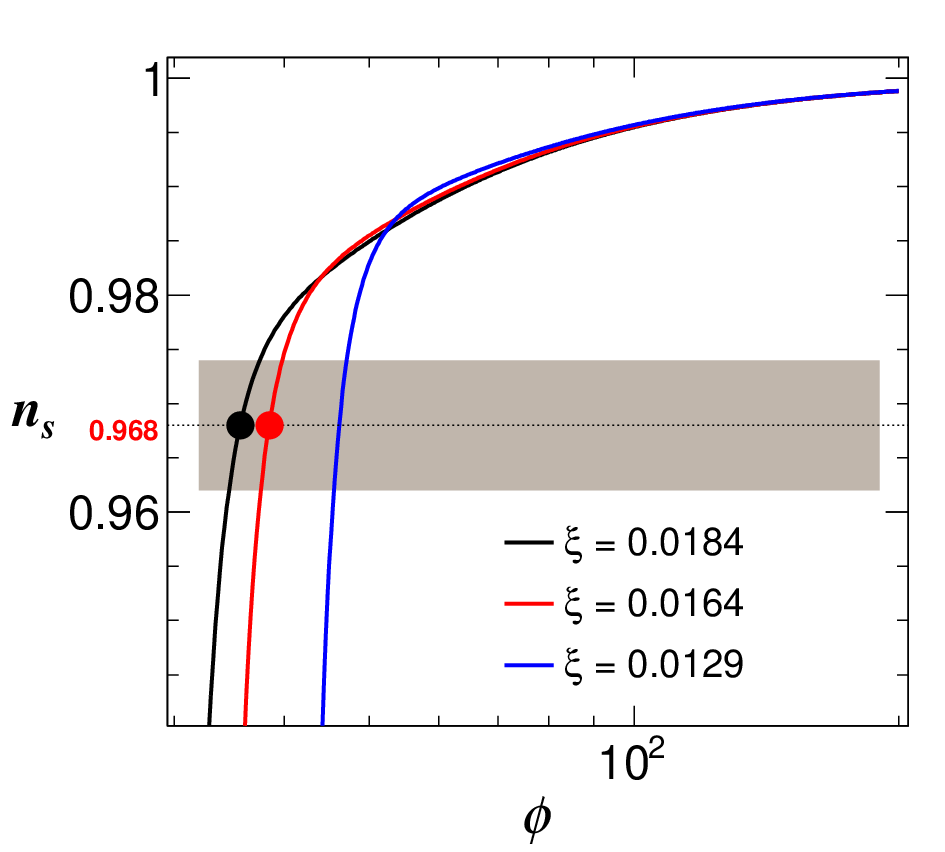


For visualization of variation of the tensor-to-scalar ratio and the scalar spectral index with respect to the inflaton field as well as the variation of with respect to , we may do the numerical calculations by substituting the equations (61) and (62) in equations (52) and substituting equation (61) in the equation (57) for different values of non-minimal coupling parameter . The values of the parameter are decided on the basis of bounds of data of and as mentioned above. The results of these calculations are shown in the Fig.5. It is seen that as the constraint set by the Planck’s data on , according to the upper bounds of given by the Planck and BICEP2/Keck experiments, the actual value of should lies below the values of the same for and respectively. Moreover, the BICEP2/Keck’s data on upper bound of lies well within the and confidence level (c.l.) contours obtained from Planck’s data. We found that under the same constraint, the lower bound of c.l. contour is obtained for the value of (see the top left plot of the Fig.5). This indicates that the most probable value of should lie within .
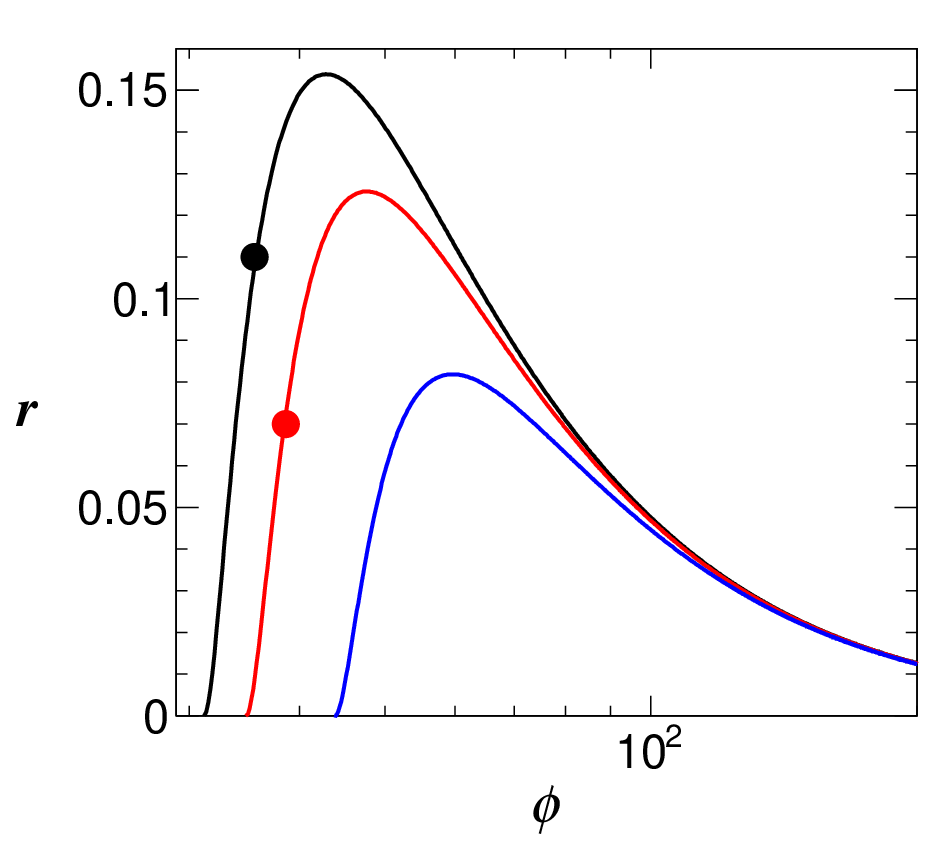
The values of corresponding to data points in the plot (top middle plot of the Fig.5) are guided to draw the same points in the plot (top right plot of the Fig.5). These values of are and corresponding to upper bounds of Planck’s () and BICEP2/Keck’s () data respectively. From these two values of , we see that Planck’s and BICEP2/Keck’s bounds on are closed in the inflationary phases.
It is also clear from the plot that the value of is maximum () at a particular value of (). However, both data points lie at initial phases than , such that smaller the value of data point with smaller , the phase of would be slightly more initial than corresponding . Thus data points in plot may be considered as the average value of over a certain range of including for the concerned value of . The upper bounds of BICEP2/Keck’s and Planck’s data on are found to be the average values of over and distributions of with respect to for and respectively (see the bottom plots of the Fig.5). Therefore during the inflation, the evolution of from to (at the end of inflation) should always contains the value , where reaches its maximum value before starts to decrease. Moreover, the average values of over whole distributions for and are and respectively. Both these values of lie within the upper bounds set by the Planck and BICEP2/Keck collaboration.
It should be noted that upto certain initial value of the inflaton field , the inflation is not well defined (giving random and large values and ) due to the reason discussed in the previous section related to the masses of the scalar fields. From the potential (45) this required initial value of can be found as . Thus the initial or the minimum values of from which the inflation is found to be well defined for , and are , and respectively. From this initial value of depending on the value of , the potential (45) becomes positive and sufficiently flat, and consequently the mass squared of all fields (, , and ) remain positive favouring for the slow-roll approximation to the inflation dynamics. Again, we take that value of as end value at which the value of becomes equal to , and both and become independent of the parameter . We found this end value of . So, our range of lies between the initial value (for a particular ) and the end value.
5.2 Number of e-foldings
To see what are the values of e-foldings that are related with the values of inflaton field corresponding to upper bounds of tensor-to-scalar ratio set by different experiments as mentioned above, we have derived the expression for the number of e-foldings [6] given by the potential (45) as
| (65) |
where
and as discussed in the previous subsection is the critical value of below which (specially) the field becomes unstable due to tachyonic instability (). As mentioned there, these critical values of are , and for , and respectively. The equation (65) also shows that for a physically acceptable value of , should be greater than . This is obvious because at the potential becomes just positive as mentioned earlier.
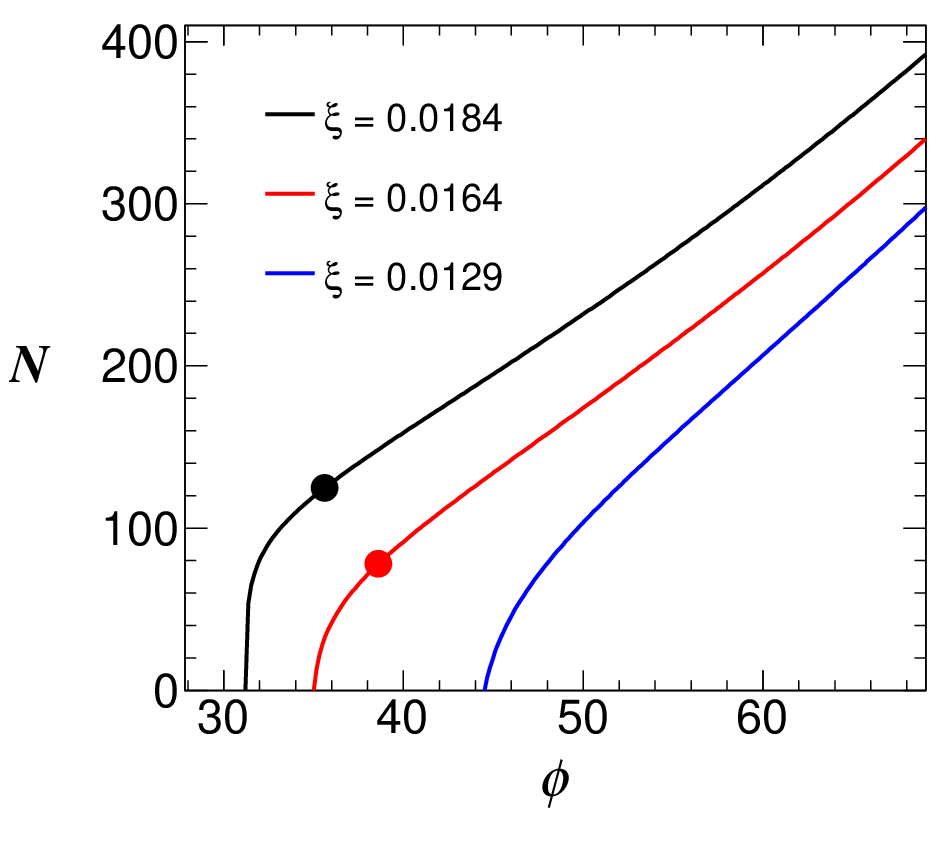
The numerical calculations using the equation (65) give that the upper bounds of from the BICEP2/Keck and the Planck experiments correspond to and e-foldings with and respectively (see the Fig.6). It is clear that the smaller value of or gives smaller value of number of e-foldings for all values of . Yet, it is difficult to infer something from the prediction of number of e-foldings by the potential using this analysis. However, it is certain that the model could predict a sufficient number of e-foldings () for upper bounds of set by the BICEP2/Keck and the Planck experiments. The number of e-foldings is required for any model of inflation to be valid [6]. Our model’s prediction in terms of the number of e-foldings is discussed in the subsection 5.6 below.
5.3 Relations between , and
Numerical calculations are done on the equation (60) using equations (61) and (62) via equations (52) and (57) to see the variation of the running of the tensor spectral index as a function of the tensor-to-scalar ratio and the field for different values of the parameter corresponding to experimental upper bounds on as mentioned above. The model independent numerical calculation is also done using equation (60) for values of from to . The results of all these calculations are shown in the Fig.7. The model independent curve is found to passages through points on model based curves for different (see the left plot of Fig.7). These points give the values of corresponding to experimental upper bounds on (refer to previous section). This suggests that the values of for and lie within the upper bounds of BICEP2/Keck’s and Planck’s data respectively. From this result we may say that the slow-roll approximation imposed on our model is appropriate. Furthermore, the value of for the upper bound of BICEP2/Keck’s data is found to lies well within the and c.l. contours drawn on the basis Planck’s data. Hence, the most probable value of the non-minimal coupling parameter should lie within . This is the same inference as we have drawn above.

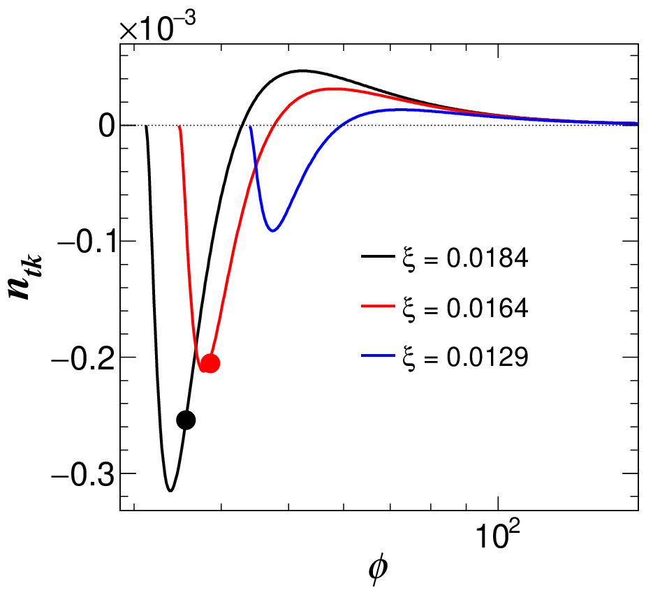
is appeared to has oscillatory nature from negative to positive value with increasing value of (see the right plot of the Fig.7). But the oscillation is asymmetric, as it is seen that the amplitude of the oscillatory curve on negative side is very large in comparison to its positive counterpart. Thus on average, each curve will give negative value of for a particular value of . Comparison with the top right plot of the Fig.5 it is clear that at , reaches to its zero value. This is because, the represents the second harmonics of the tensor power spectrum, whereas represents its principal harmonics. attains its minimum negative value at a particular value of during its initial stage of evolution in the inflation phase. Almost at or near to this stage, the values of for and lie within the upper bounds of BICEP2/Keck’s and Planck’s data respectively. The values of corresponding to both these experimental limits of are same as mentioned earlier.
5.4 Relations between , and
For the same purpose as in the previous cases, numerical calculation was done on by using the generic equation (54) via equations (61), (62) and (63) for different values of as in the earlier cases, the results of which are shown in the Fig.8.


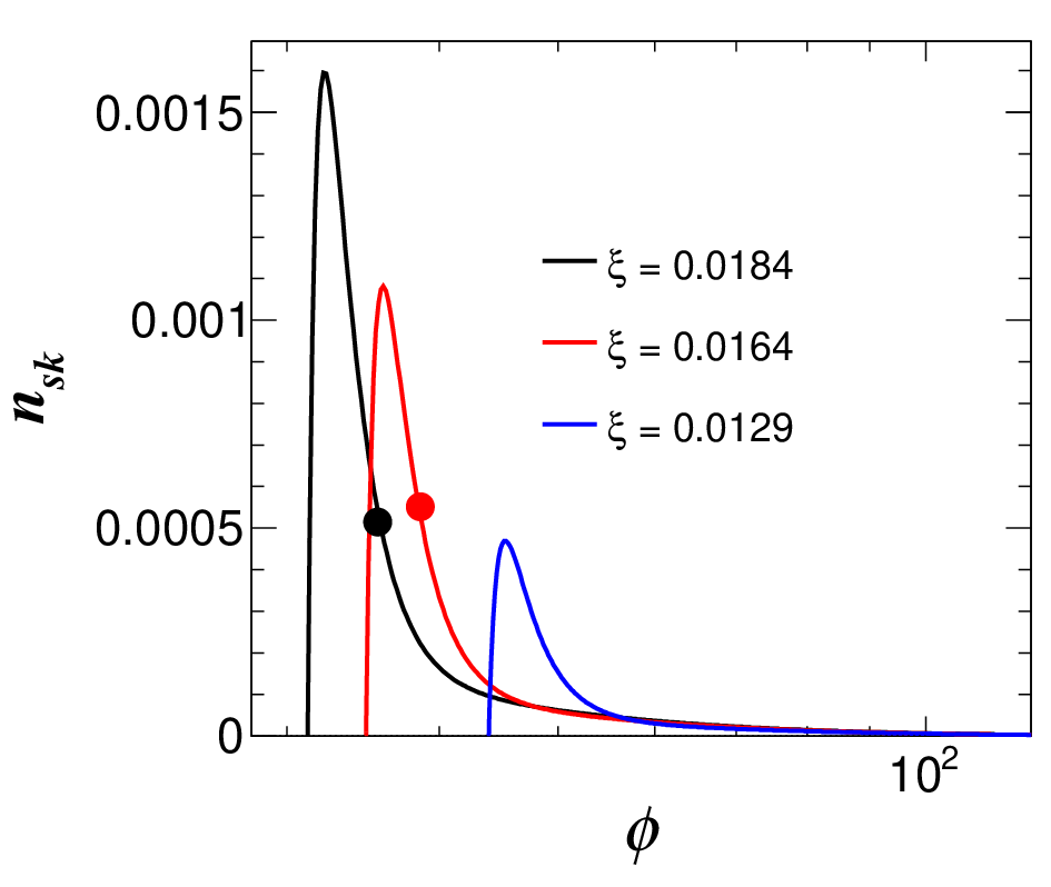
We found that the upper bounds of BICEP2/Keck’s and Planck’s data give that should take values within and respectively. From these results we used the upper bounds of corresponding to the upper bounds of to establish a numerical relation among , and as given by
| (66) |
It is observed that as in the case of , the model independent values of for to obtained from the equation (66), passage through different points on the model based curves depending on the values of (see the left plot of Fig.8). These points correspond to the results for upper limits of observed value of as already mentioned. Thus same inference can be made from plot together with plot as in the case of previous plot of the Fig.7 as well as in the case of plot of the Fig.5. That is, our model could incorporate both experimental upper limits of as well as the experimental value of within a specific range of values of the non-minimal coupling parameter . The value of obtained for the upper bound of BICEP2/Keck’s data is found to lie well within the c.l. contour, drawn as mentioned earlier, in the plot. However in the plot, the value of obtained for the upper bound of Planck’s data is also found to lie within the c.l. contour. Hence, we may infer from here also that the most probable value of should lie within .
As in the case of plot of the Fig.5, the value of
becomes maximum () at a particular value of ().
But this happens in a earlier phase of for this case than plot
and accordingly data points are shifted away from to retain their
position over the specified values of as mentioned earlier. Hence,
there is a reasonable (and should be observable) phase
difference between the values of and . It is mainly due to the
factor that remains effective in the equation of as
clear from the numerical equation (66). Taking the
reference of plot, we have found that the values for upper
bounds of BICEP2/Keck’s and Planck’s data correspond to and
of total values of curves for and
respectively. Thus should be contained in the
process of evolution of during the inflation as in the case of
.
Again, comparing with the plot of the the Fig.5,
it can be seen that where the value of remains as constant
(maximum ), there the values of is zero. Moreover, with higher
values of as the values of increase very fast at slightly earlier
phases of than that with the lower values of , so also
increases with similar fashion, but with a prominent manifestation. These
corresponding behaviours of and
with respect to are due to the fact that
is the principal harmonics of the scalar power spectrum and is the running of
.
5.5 Relations between , and
Finally, to study the behaviours of with respect to , and we have to do the numerical calculations using the generic expression (55) via equations (61), (62), (63) and (64). The results of these calculations are shown in the Fig.9 for different values as in the earlier cases. It is found that as per the upper bounds of the BICEP2/Keck’s and Planck’s data of , the actual value of should lie within the ranges of and respectively.
Similar to the case of , we derived a model independent relation for the also in terms of and from the numerical data in the form:
| (67) |
Same inference can be made from this equation as that is made from the equation (66). Moreover, this equation indicates that the probable value of should be negative for any value of other than zero or . Here the later limit of sets a constraint that the value of can not be greater than . This is in agreement with the constraint set by the model independent equation (60) that for the value of should remain as negative the value of should be less than . Again, comparatively a more squeezed constraint on is set by the equation (66) is that for the value of to be remain positive the value of should be less than . These constraints on definitely rule out the reported BICEP2 experiment [11] data on .


From the and plots a similar conclusion can be drawn on the value of non-minimal coupling parameter , i.e. on the model prediction as in the previous cases.
Moreover, the values of oscillate in between positive to negative values with the increasing values of and as represents the second harmonics of scalar power spectrum. Hence at , the value of is found to be zero (refer to the Fig.8 and Fig.9). Due to this fact, points corresponding to the data on plot are shifted towards minimum negative side.
Thus, our model could predict all conventional observables of the slow-roll approximation of inflation corresponding to the experimental bounds of the tensor-to-scalar ratio as well as to the Planck’s precise experimental value of scalar spectral index as mentioned above. The corresponding predicted values of the inflaton field are found to be same for all observables.
Furthermore, it is worthy to mention that although the equation (60) is based on the model independent derivation, but the equations (66) and (67) are derived from numerical results obtained from our model. Thus equations (66) and (67) can be used explicitly to test our model from future cosmological observations.
5.6 Observables in terms of number of e-foldings
In order to compare our model’s predictions precisely with other models as well as with observations, it is necessary to calculate the observables of slow-roll parameters in terms of number of e-foldings. For this purpose, we have to solve the equation (65) of the number of e-foldings () to obtain the inflaton field as a function of . As this equation is very complex to find such a solution, we may simplify it by neglecting its second and 3rd terms. This simplification is justified by the fact that the contributions of these two terms to the value of are found to be very negligible in comparison to other two terms from the numerical calculation for the range of values of we have considered. The second term contribute only and the third term only on average to the sum of the contributions made by the first and fourth terms. Thus with this simplification, the field can be obtained from the equation (65) approximately as
| (68) |
where and represent the same expression as given in the subsection 5.2 and . As mentioned earlier, for physically acceptable value of (or ) .
Now, the values of , , , and can be obtained in terms of the number of e-foldings for a given value of by substituting the equation (68) into the the respective equations (57), (52), (53), (54) and (55) via equations (61), (62), (63) and (64).
Presently, it is almost universally accepted that the number of e-foldings before the end of inflation were . So in our calculation we have taken three values of number of e-foldings, viz., by widening the e-folding window in the upper side by one decade value. Moreover, from above analysis it is clear that the most probable value of non-minimal coupling parameter should be laid within . Hence, under the constraints of and the Planck’s data of , for this calculation also we have taken three values of , and . Also taking into account of values of the for the experimental upper limits of as mentioned in the earlier occasions, we set the values of in this particular numerical calculation. Table 1 shows the estimated values of different observables obtained from our model for the said values of and .
It is seen from the table 1 that, the values of the tensor-to-scalar ratio estimated from our model for the number of e-foldings = with non-minimal coupling parameter = , and lie well below the upper limits set by Planck ( at c.l.) [9, 10] and BICEP2/Keck ( at c.l.) [12] collaborations. Similarly, the estimated values of the scalar spectral index from our model for these parameters are seen to be very close to the latest value of ( at c.l.) as measured by the Planck collaboration [10] (in fact for = and almost all values of are laying within the range of data). Particularly, the value of for = with = is in agreement with the mean value of the Planck’s data (see the Fig.10 also). Within both these observables and increase in their magnitudes with increasing value of . The general behaviours of all observables with respect to and are shown in the Fig.10.


6 Summary and conclusions
We have found that the idea of supersymmetric hybrid inflation with non-minimal coupling to gravity is very interesting and useful, because the simplest version of the model based on it can accommodate the upper limits for the tensor-to-scalar ratio set by the Planck and BICEP2/Keck experiments for the values of non-minimal coupling parameter and respectively. The values of for and , restricted by the Planck’s data on , fall within the range of upper bounds of the BICEP2/Keck’s and the Planck’s data respectively. Within these ranges of data as well as the said ranges of parameter , the expected values of the running of the tensor spectral index , scalar spectral index and its running are found to belong. The values of the inflaton field corresponding to all these observables are found to be , and respectively for upper bound of BICEP2/Keck’s data and upper bound of Planck’s data. The number of e-foldings corresponding to these values of are found to be as expected. The and confidence level predictions based on the Planck’s data for all the said observables indicate that the most probable value of for our model should lie within . Implying that the coupling is very week. More precisely, from the calculations using the number of e-foldings, the values of estimated from our model for and for number of e-foldings are laying well below the upper limits set by the Planck and BICEP2/Keck collaborations. Similarly, for the said parameters, the values of estimated from our model are in good agreement with its latest Planck data, specially the agreement is excellent for = with . Moreover, these estimated values of and are also found to be in agreement with the results of the Ref. [51]. Therefore, the most probable value of the non-minimal coupling parameter is found to be .
Thus, this type of model can be used to predict a wide range of observational data on the cosmic inflation. So, it would be interesting to see the predictions of observables of the cosmic inflation by other versions of such model in future. In this context, it should be noted that the running of the scalar spectral index can be considered as a probe of both inflation itself, and of the overall evolution of the very early universe as its magnitude is relatively consistent in comparison to tensor amplitude [64]. It is potentially detectable by future large scale observations through measurements of clustering of high-redshift galaxy surveys together with CMB data or the 21 cm forest signal observations [64]. In the event of such measurements, our model of non-minimal coupling of gravity with SUSY hybrid inflation will play a significant role.
The constrained equation for the running of the tensor spectral index (equation (60)) is derived independent of any model. However, such equations for the running of the scalar spectral index and its running (equations (66) and (67) respectively) are derived numerically based on the structure of our model. All these equations can be used as constraint equations of slow-roll approximation. Specially, the equation (60) can be used to test slow-roll approximation itself, and equations (66) and (67) can be used to test our model from the data of future cosmological observations.
Lastly, it is necessary to mention that to avoid the negative potential of the inflaton field of our model within the effective range of inflation, we introduced a second order non-minimal coupling parameter along with the coupling parameter into the superconformal factor . For simplified formulations and calculations we consider a very effective relation between and as . It is already clear that this relationship works very well for our model. However, there may exists other such possible relations also.
Acknowledgments
The author is thankful to the Inter-University Centre for Astronomy and Astrophysics (IUCAA), Pune for hospitality during his visits as a Visiting Associate of the institute.
References
- (1) A. A. Starobinsky, A new type of isotropic cosmological models without singularity, Phys. Lett. B 91 (1980) 99.
- (2) D. Kazanas, Dynamics of the universe and spontaneous symmetry breaking, Astrophys. J. Lett. 241 (1980) L59.
- (3) A. H. Guth, Inflationary universe: A possible solution to the horizon and flatness problems, Phys. Rev. D 23 (1981) 347.
- (4) K. Sato, First-order phase transition of a vacuum and the expansion of the Universe, Mon. Not. R. Astron. Soc. 195 (1981) 467.
- (5) K. Sato, Cosmological baryon-number domain structure and the first order phase transition of a vacuum, Phys. Lett. B 99 (1981) 66.
- (6) B. A. Bassett, S. Tsujikawa and D. Wands, Inflation dynamics and reheating, Rev. Mod. Phys. 78 (2000) 537 [arXiv:astro-ph/0507632].
- (7) J. Martin, C. Ringeval and V. Vennin, Encyclopedia Inflationaris, Phys. Dark Univ. 5-6 (2014) 75 [ArXiv:1303.3787].
- (8) C. L. Bennett et al., 4-Year COBE DMR Cosmic Microwave Background Observations: Maps and Basic Results, Astrophys. J. 464 (1996) L1 [arXiv:astro-ph/9601067].
- (9) P. A. R. Ade et al. (Planck Collaboration), Planck 2013 results. XVI. Cosmological parameters, A&A 571 (2014) A16 [arXiv:1303.5076].
- (10) P. A. R. Ade et al. (Planck Collaboration), Planck 2015 results. XIII. Cosmological parameters, A&A 594 (2016) A13 [arXiv:1502.01589].
- (11) P. A. R. Ade et al. (BICEP2 Collaboration), BICEP2 I: Detection Of B-mode Polarization at Degree Angular Scales, Phys. Rev. Lett. 112 (2014) 241101 [arXiv:1403.3985].
- (12) P. A. R. Ade et al. (Keck Array and BICEP2 Collaborations), BICEP2 / Keck Array VI: Improved Constraints On Cosmology and Foregrounds When Adding 95 GHz Data From Keck Array, Phys. Rev. Lett. 116 (2016) 031302 [arXiv:1510.09217].
- (13) G. Hinshaw et al. [WMAP Collaboration], Nine-Year Wilkinson Microwave Anisotropy Probe (WMAP) Observations: Cosmological Parameter Results, Astrophys. J. Suppl. 208 (2013) 19 [arXiv:1212.5226].
- (14) A. Linde, Chaotic inflation, Phys. Lett. B 129 (1983) 177.
- (15) A. D. Linde, Hybrid Inflation, Phys. Rev. D 49 (1994) 748 [arXiv:astro-ph/9307002].
- (16) E. J. Copeland, A. R. Liddle, D. H. Lyth, E. D. Stewart and D. Wands, False vacuum inflation with Einstein gravity, Phys. Rev. D 49 (1994) 6410 [arXiv:astro-ph/9401011].
- (17) M. Kawasaki, M. Yamaguchi and T. Yanagida, Natural Chaotic Inflation in Supergravity, Phys. Rev. Lett. 85 (2000) 3572 [arXiv:hep-ph/0004243].
- (18) J. L. Feng, Naturalness and the Status of Supersymmetry, Annual Rev. Nucl. Part. Sci. 63 (2013) 351 [arXiv:1302.6587].
- (19) L. E. Mendes and A. R. Liddle,Initial conditions for hybrid inflation, Phys. Rev. D 62 (2000) 103511 [arXiv:astro-ph/0006020].
- (20) D. H. Lyth and A. Riotto, Particle Physics Models of Inflation and the Cosmological Density Perturbation, Phys. Rep. 314 (1999) 1 [arXiv:hep-ph/9807278].
- (21) D. Carmi, A. Falkowski, E. Kuflik, T. Volansky, J. Zupan, Higgs After the Discovery: A Status Report, JHEP 10 (2012) 196 [arXiv:1207.1718].
- (22) S. Ferrara, R. Kallosh, A. Linde, A. Marrani and A. Van Proeyen, Superconformal Symmetry, NMSSM, and Inflation, Phys. Rev. D83 (2011) 025008 [arXiv:1008.2942].
- (23) S. Ferrara, R. Kallosh, A. Linde, A. Marrani and A. Van Proeyen, Jordan Frame Supergravity and Inflation in NMSSM, Phys. Rev. D 82 (2010) 045003 [arXiv:1004.0712].
- (24) H. M. Lee, Chaotic inflation in Jordan frame supergravity, JCAP 08 (2010) 003 [arXiv:1005.2735].
- (25) D. S. Salopek, J. R. Bond and J. M. Bardeen, Designing density fluctuation spectra in inflation, Phys. Rev. D 40 (1989) 1753.
- (26) T. Futamase and K.-i. Maeda, Chaotic inflationary scenario of the Universe with a nonminimally coupled ”inflaton” field, Phys. Rev. D 39 (1989) 399.
- (27) R. Fakir and W.G. Unruh, Improvement on cosmological chaotic inflation through nonminimal coupling, Phys. Rev. D 41 (1990) 1783.
- (28) S. Mukaigawa, T. Muta, S. D. Odintsov, Finite Grand Unified Theories and Inflation, Int. J. Mod. Phys. A 13 (1998) 2739 [arXiv:hep-ph/9709299].
- (29) F. L. Bezrukov and M. Shaposhnikov, The Standard Model Higgs boson as the inflaton, Phys. Lett. B 659 (2008) 703 [arXiv:0710.3755].
- (30) A. O. Barvinsky, A. Y. Kamenshchik and A. A. Starobinsky, Inflation scenario via the Standard Model Higgs boson and LHC, JCAP 11 (2008) 021 [arXiv:0809.2104].
- (31) F. Bezrukov and M. Shaposhnikov, Standard Model Higgs boson mass from inflation: two loop analysis, JHEP 07 (2009) 089 [arXiv:0904.1537].
- (32) F. Bezrukov, D. Gorbunov and M. Shaposhnikov, On initial conditions for the Hot Big Bang, JCAP 06 (2009) 029 [arXiv:0812.3622].
- (33) J. G.-Bellido, D. G. Figueroa and J. Rubio, Preheating in the Standard Model with the Higgs-Inflaton coupled to gravity, Phys. Rev. D 79 (2009) 063531 [arXiv:0812.4624].
- (34) A. D. Simone, M. P. Hertzberg and F. Wilczek, Running Inflation in the Standard Model, Phys. Lett. B 678 (2009) 1 [arXiv:0812.4946].
- (35) A. O. Barvinsky, A. Y. Kamenshchik, C. Kiefer, A. A. Starobinsky and C. Steinwachs, Asymptotic freedom in inflationary cosmology with a non-minimally coupled Higgs field, JCAP 12 (2009) 003 [arXiv:0904.1698].
- (36) A. O. Barvinsky, A. Y. Kamenshchik, C. Kiefer, A. A. Starobinsky and C. Steinwachs, Higgs boson, renormalization group, and naturalness in cosmology, Euro. Phys. J. C 72 (2012) 2219 [arXiv:0910.1041].
- (37) F. Bezrukov, A. Magnin, M. Shaposhnikov and S. Sibiryakov, Higgs inflation: consistency and generalisations, JHEP 01 (2011) 016 [arXiv:1008.5157].
- (38) S. Choudhury, T. Chakraborty and S. Pal, Higgs inflation from new Kähler potential, Nucl. Phys. B 880 (2014), 155 [arXiv:1305.0981].
- (39) A. Linde, M. Noorbala and A. Westphal, Observational consequences of chaotic inflation with nonminimal coupling to gravity, JCAP 03 (2011) 013 [ArXiv:1101.2652].
- (40) E. Elizalde, S. D. Odintsov, E. O. Pozdeeva and S. Yu. Vernov, Renormalization-group inflationary scalar electrodynamics and SU(5) scenarios confronted with Planck2013 and BICEP2 results, Phys. Rev. D 90 (2014) 084001 [arXiv:1408.1285].
- (41) T. Inagaki, R. Nakanishi and S. D. Odintsov, Inflationary Parameters in Renormalization Group Improved Theory, Astrophys. Space Sci. 354 (2014) 2108 [arXiv:1408.1270].
- (42) T. Inagaki, R. Nakanishi and S. D. Odintsov, Non-Minimal Two-Loop Inflation, Phys. Lett. B 745 (2015) 105 [arXiv:1502.06301].
- (43) R. Myrzakulov, S. Odintsov and L. Sebastiani, Inflationary universe from higher derivative quantum gravity coupled with scalar electrodynamics, Nucl. Phys. B 907 (2016) 646 [arXiv:1604.06088].
- (44) E. Elizalde, S. D. Odintsov, E. O. Pozdeeva and S. Y. Vernov, Cosmological attractor inflation from the RG-improved Higgs sector of f inite gauge theory, JCAP 02 (2016) 025 [arXiv:1509.08817].
- (45) R. Kallosh and A. Linde, New models of chaotic inflation in supergravity, JCAP 11 (2010) 011 [ArXiv:1008.3375].
- (46) D. I. Kaiser and A. T. Todhunter, Primordial Perturbations from Multifield Inflation with Nonminimal Couplings, Phys. Rev. D 81 (2010) 124037 [arXiv:1004.3805].
- (47) D. I. Kaiser, E. A. Mazenc and E. I. Sfakianakis, Primordial Bispectrum from Multifield Inflation with Nonminimal Couplings, Phys. Rev. D 87 (2013) 064004 [arXiv:1210.7487].
- (48) R. N. Greenwood, D. I. Kaiser and E. I. Sfakianakis, Multifield Dynamics of Higgs Inflation, Phy. Rev. D 87 (2013) 064021 [arXiv:1210.8190].
- (49) D. I. Kaiser and E. I. Sfakianakis, Multifield Inflation after Planck: The Case for Nonminimal Couplings, Phys. Rev. Lett. 112 (2014) 011302 [arXiv:1304.0363];
- (50) K. Schutz, E. I. Sfakianakis and D. I. Kaiser, Multifield Inflation after Planck: Isocurvature Modes from Nonminimal Couplings, Phys. Rev. D 89 (2014) 064044 [arXiv:1310.8285].
- (51) G. Lazarides and C. Pallis, Shift Symmetry and Higgs Inflation in Supergravity with Observable Gravitational Waves, JHEP 1511 (2015) 114 [arXiv:1508.06682];
- (52) C. Pallis, Kinetically modified nonminimal Higgs inflation in supergravity, Phys. Rev. D 92 (2015) 121305 [arXiv:1511.01456].
- (53) A. Mazumdar and J. Rocher, Particle physics models of inflation and curvaton scenarios, Phys. Rep. 497 (2011) 85 [arXiv:1001.0993].
- (54) G. Dvali, Q. Shafi and R. Schaefer, Large Scale Structure and Supersymmetric Inflation without Fine Tuning, Phys. Rev. Lett. 73 (1994) 1886 [arXiv:hep-ph/9406319].
- (55) S. Orani and A. Rajantie, Supersymmetric hybrid inflation with a light scalar, Phys. Rev. D 88 (2013) 043508.
- (56) K. Das, V. Domcke and K. Dutta, Supergravity Contributions to Inflation in models with non-minimal coupling to gravity, JCAP 03 (2017) 036 [arXiv:1612.07075].
- (57) R. Kallosh, L. Kofman, A. D. Linde and A. Van Proeyen, Superconformal Symmetry, Supergravity and Cosmology, Class. Quant. Grav. 17 (2000) 4269 [Erratum-ibid 21 (2004) 5017] [arXiv:hep-th/0006179].
- (58) E. Cremmer, B. Julia and J. Scherk, S. Ferrara, L. Girardello and P. van Nieuwenhuizen, Spontaneous symmetry breaking and Higgs effect in supergravity without cosmological constant, Nucl. Phys. B 147 (1979) 105.
- (59) E. Cremmer, S. Ferrara, L. Girardello and A. Van Proeyen, Yang-Mills theories with local supersymmetry: Lagrangian, transformation laws and superHiggs Effect, Nucl. Phys. B 212 (1983) 413.
- (60) M. Civiletti, C. Pallis and Q. Shafi,Upper Bound on the Tensor-to-Scalar Ratio in GUT-Scale Supersymmetric Hybrid Inflation, Phys. Lett. B 733 (2014) 276 [arXiv:1402.6254].
- (61) T. Kobayashi and O. Seto, Beginning of Universe through large field hybrid inflation, Mod. Phys. Lett. A 30 (2015) 1550106 [arXiv:1404.3102].
- (62) G. Felder, A. Frolov, L. Kofman and A. Linde, Cosmology with negative potentials, Phys. Rev. D 66 (2002) 023507 [arXiv:hep-th/0202017]
- (63) M. C.-González, G. German, A. H.-Aguilar, J. C. Hidalgo, R. Sussman, Testing Hybrid Natural Inflation with BICEP2, Phys. Lett. B 734 (2014) 345 [arXiv:1404.1122].
- (64) P. Adshead, R. Easther, J. Pritchard and A. Loeb, Inflation and the Scale Dependent Spectral Index: Prospects and Strategies, JCAP 1102 (2011) 021 [arXiv:1007.3748].