跳到论文正文
W Papers独立论文阅读器 arXiv:1705.05358 论文正文 计算阅读时间 · 0%
引用这篇论文根据当前论文元数据生成,正式投稿前建议核对。


License: arXiv.org perpetual non-exclusive license
arXiv:1705.05358v2 [hep-ph] 06 Jun 2017

Construction of lepton mass matrices and TeV-scale phenomenology in the minimal left-right symmetric model

Chang-Hun Lee Affiliation: Maryland Center for Fundamental Physics and Department of Physics,
University of Maryland, College Park,
Maryland 20742, U.S.A.
Email: changhun@terpmail.umd.edu
Abstract

We develop a systematic procedure of constructing lepton mass matrices that satisfy all the experimental constraints in the light lepton sector of the minimal left-right symmetric model with type-I seesaw dominance. This method is unique since it is applicable to the most general cases of type-I seesaw with complex electroweak vacuum expectation values in the model. With this method, we investigate the TeV-scale phenomenology in the normal hierarchy without fine-tuning of model parameters, focusing on the charged lepton flavour violation, neutrinoless double beta decay, and electric dipole moments of charged leptons. We examine the predictions for typical ranges of associated observables such as branching ratios of rare lepton decays, and study how those experimental constraints affect the model parameter space. The most notable result is that the regions of parameter space that allow small light neutrino masses have been constrained by the present experimental bounds from charged lepton flavour violation. Furthermore, we also find that the mass of the lightest heavy neutrino should be relatively small in order to satisfy those experimental constraints.

1 Introduction

The Standard Model (SM) of particle physics is a chiral theory with a broken parity symmetry, and the left-right symmetric model is an extension of the SM with the parity symmetry restored at high energies [1, 2, 3]. Its extended particle content (e.g. right-handed (RH) neutrinos and gauge bosons) allows us not only to find the solution to the parity problem of the SM but also to solve the problem of understanding the neutrino masses via the seesaw mechanism [4, 5, 6, 7]. If the scale of parity restoration is in the few TeV range, we can expect new physics signals that are not present in the SM in planned future experiments. For example, since the lepton number for each flavour in the left-right symmetric model is no longer an exact symmetry of nature as in the SM, it is possible to observe charged lepton flavour violation (CLFV) processes such as μ→e​γ\mu\to e\gamma or lepton number violation effects through neutrinoless double beta decay (0​ν​β​β0\nu\beta\beta). Furthermore, since the left-right symmetric model not only has more particles but also has more sources of CP violation not present in the SM such as complex Yukawa couplings and vacuum expectation values (VEV), we can also expect large CP violating effects such as the electric dipole moment (EDM) of a charged lepton. In this paper, these aspects of the left-right symmetric model will be discussed.

In the lepton sector of the minimal left-right symmetric model (MLRSM), of which a brief review is provided in section 2, we have four mass matrices: the charged lepton mass matrix MℓM_{\ell}, the Dirac neutrino mass matrix MDM_{D}, and the left-handed and RH Majorana neutrino mass matrices MLM_{L} and MRM_{R}. The light neutrino mass matrix MνM_{\nu} is determined by MDM_{D}, MLM_{L}, and MRM_{R} through the seesaw mechanism Mν≈ML−MD​MR−1​MD𝖳M_{\nu}\approx M_{L}-M_{D}M_{R}^{-1}M_{D}^{\mathsf{T}}. Since we have experimental data on the masses of charged leptons and the squared-mass differences of neutrinos as well as their mixing angles, MℓM_{\ell} is completely known in the charged lepton mass basis and MνM_{\nu} is also partially determined in its own mass basis and in the charged lepton mass basis. The neutrino mass matrices MDM_{D}, MLM_{L}, and MRM_{R} are nonetheless completely unknown, and constructing those matrices compatible with experimental data is a nontrivial problem, not only because MℓM_{\ell} and MDM_{D} in the MLRSM are determined from common Yukawa couplings and electroweak VEV’s, but also because those Yukawa coupling matrices have a specific structure (i.e. Hermitian or symmetric) in a specific basis (i.e. symmetry basis) due to the discrete symmetry (i.e. parity or charge conjugation symmetry) of the model that realizes the manifest left-right symmetry at high energies.

For simplicity, we may assume that the electroweak VEV’s are all real, in which case MℓM_{\ell} and MDM_{D} have the same structure (i.e. Hermitian or symmetric) as the Yukawa coupling matrices. Since they maintain that structure in any basis, we can work in the charged lepton mass basis where MℓM_{\ell} is completely determined so that we can practically forget about it while keeping the structure of mass matrices. Now using that structure itself, we can find MRM_{R} from known MDM_{D} [8] or alternatively find MDM_{D} from known MRM_{R} [9]. Without loss of generality, however, we can make only one of two electroweak VEV’s real by gauge transformation. Furthermore, for the TeV-scale MLRSM, MDM_{D} assumed or constructed in such ways usually requires fine-tuning of Yukawa couplings and VEV’s, and it would be rather difficult to make natural predictions for the TeV-scale phenomenology of the MLRSM using those mass matrices.

In this paper, we develop a different approach appropriate for the case of type-I dominance (i.e. ML=0M_{L}=0) with complex electroweak VEV’s: (i) the Yukawa coupling matrices with a desired structure are constructed from MℓM_{\ell} in the symmetry basis; (ii) MDM_{D} is determined from those Yukawa couplings as well as the electroweak VEV’s, and MRM_{R} is calculated from MDM_{D} we have found. Since Yukawa couplings are explicitly constructed and MDM_{D} is calculated from them, fine-tuned MDM_{D} can only appear rarely. With this method, we collect a huge amount of data points that satisfy all the major experimental constraints, and conduct a comprehensive study of the TeV-scale phenomenology of the model, focusing on the CLFV, 0​ν​β​β0\nu\beta\beta, and EDM’s of charged leptons.

There are several works which studied CLFV and 0​ν​β​β0\nu\beta\beta in the MLRSM: in reference [10], those effects were discussed in the type-I or type-II seesaw dominance, and several processes of 0​ν​β​β0\nu\beta\beta were examined in detail; in reference [11], CLFV and 0​ν​β​β0\nu\beta\beta processes were investigated also in type-I or type-II dominance with emphasis on the allowed masses of doubly charged scalar fields; in reference [12], the type-I+II seesaw contributions were simultaneously considered as in references [8] and [9], but with richer results on the phenomenology; in reference [13], the CLFV effects were studied in detail also in the type-I+II seesaw cases by a slightly different method from the one originally proposed by reference [8]. However, the common features of those works are: (i) real electroweak VEV’s were explicitly or implicitly assumed, and (ii) MDM_{D} or MRM_{R} was chosen for numerical analysis without considering the issue of fine-tuning. Even though we can still obtain meaningful results focusing on specific regions of parameter space with rich phenomenologies, it is important to investigate the predictions of the model in a more natural situation. Furthermore, some works assumed that the tree-level contribution to μ→e​e​e\mu\to eee is always dominant over the type-I contribution in their analyses. We will also see that this is an inadequate assumption.

This paper is organized as follows: in section 2, a brief review on the MLRSM is provided; in section 3, we systematically construct lepton mass matrices that satisfy the experimental constraints in the light lepton sector; in section 4, the conditions for the TeV-scale MLRSM is investigated, and its phenomenology is studied; all the expressions of observables of CLFV, 0​ν​β​β0\nu\beta\beta, and EDM’s of charged leptons used in this paper are summarized in appendix A; the benchmark model parameters and their predictions are provided in appendix B.

2 Minimal left-right symmetric model

In this section, we briefly review the MLRSM. The gauge group of the MLRSM is

SU​(2)L⊗SU​(2)R⊗U​(1)B−L,\displaystyle\text{SU}(2)_{L}\otimes\text{SU}(2)_{R}\otimes\text{U}(1)_{B-L}, (1)

and the representations of the leptons are

LL​i′=(νL​i′ℓL​i′)∼(2,1,−1),\displaystyle L_{Li}^{\prime}=\left(\begin{array}[]{c}\nu_{Li}^{\prime}\\ \ell_{Li}^{\prime}\end{array}\right)\sim(\textbf{2},\textbf{1},-1), LR​i′=(νR​i′ℓR​i′)∼(1,2,−1)\displaystyle\qquad L_{Ri}^{\prime}=\left(\begin{array}[]{c}\nu_{Ri}^{\prime}\\ \ell_{Ri}^{\prime}\end{array}\right)\sim(\textbf{1},\textbf{2},-1)

where ii is the flavour index. The bi-doublet scalar field is given by

Φ=(ϕ10ϕ2+ϕ1−ϕ20)∼(2,2,0),\displaystyle\Phi=\left(\begin{array}[]{cc}\phi_{1}^{0}&\phi_{2}^{+}\\ \phi_{1}^{-}&\phi_{2}^{0}\end{array}\right)\sim(\textbf{2},\textbf{2},0),

and the triplet scalar fields are

ΔL=(δL+/2δL+⁣+δL0−δL+/2)∼(3,1,2),ΔR=(δR+/2δR+⁣+δR0−δR+/2)∼(1,3,2).\displaystyle\Delta_{L}=\left(\begin{array}[]{cc}\delta_{L}^{+}/\sqrt{2}&\delta_{L}^{++}\\ \delta_{L}^{0}&-\delta_{L}^{+}/\sqrt{2}\end{array}\right)\sim(\textbf{3},\textbf{1},2),\qquad\Delta_{R}=\left(\begin{array}[]{cc}\delta_{R}^{+}/\sqrt{2}&\delta_{R}^{++}\\ \delta_{R}^{0}&-\delta_{R}^{+}/\sqrt{2}\end{array}\right)\sim(\textbf{1},\textbf{3},2).

The Lagrangian terms of Yukawa interactions are written as

ℒYℓ\displaystyle\mathcal{L}_{Y}^{\ell} =−LL​i′¯​(fi​j​Φ+f~i​j​Φ~)​LR​j′−hL​i​j​LL​i′c¯​i​σ2​ΔL​LL​j′−hR​i​j​LR​i′c¯​i​σ2​ΔR​LR​j′+H.c.\displaystyle=-\overline{L_{Li}^{\prime}}(f_{ij}\Phi+\tilde{f}_{ij}\tilde{\Phi})L_{Rj}^{\prime}-h_{Lij}\overline{L_{Li}^{\prime c}}i\sigma_{2}\Delta_{L}L_{Lj}^{\prime}-h_{Rij}\overline{L_{Ri}^{\prime c}}i\sigma_{2}\Delta_{R}L_{Rj}^{\prime}+\text{H.c.} (12)

where

Φ~≡σ2​Φ∗​σ2=(ϕ20∗−ϕ1+−ϕ2−ϕ10∗).\displaystyle\tilde{\Phi}\equiv\sigma_{2}\Phi^{*}\sigma_{2}=\left(\begin{array}[]{cc}\phi_{2}^{0*}&-\phi_{1}^{+}\\ -\phi_{2}^{-}&\phi_{1}^{0*}\end{array}\right).

Here, ψc≡𝖢​ψ∗\psi^{c}\equiv\mathsf{C}\psi^{*}, and thus ψc¯=−ψ𝖳​𝖢\overline{\psi^{c}}=-\psi^{\mathsf{T}}\mathsf{C} where 𝖢=i​γ2​γ0\mathsf{C}=i\gamma^{2}\gamma^{0} is the charge conjugation operator in the Dirac-Pauli representation. Note that hLh_{L} and hRh_{R} are symmetric matrices. Without loss of generality, we can write the VEV’s of scalar fields as

Φ=(κ1/200κ2​ei​α/2),ΔL=(00vL​ei​θL/20),ΔR=(00vR/20).\displaystyle\Phi=\left(\begin{array}[]{cc}\kappa_{1}/\sqrt{2}&0\\ 0&\kappa_{2}e^{i\alpha}/\sqrt{2}\end{array}\right),\qquad\Delta_{L}=\left(\begin{array}[]{cc}0&0\\ v_{L}e^{i\theta_{L}}/\sqrt{2}&0\end{array}\right),\qquad\Delta_{R}=\left(\begin{array}[]{cc}0&0\\ v_{R}/\sqrt{2}&0\end{array}\right).

After spontaneous symmetry breaking, the mass matrix of charged leptons is written as

Mℓ=12​(f​κ2​ei​α+f~​κ1),\displaystyle M_{\ell}=\frac{1}{\sqrt{2}}(f\kappa_{2}e^{i\alpha}+\tilde{f}\kappa_{1}), (21)

and the neutrino mass term is given by

ℒνmass=−12​(νL′¯​νR′c¯)​(MLMDMD𝖳MR)​(νL′cνR′)+H.c.\displaystyle\mathcal{L}_{\nu}^{\text{mass}}=-\frac{1}{2}(\overline{\nu_{L}^{\prime}}\ \overline{\nu_{R}^{\prime c}})\left(\begin{array}[]{cc}M_{L}&M_{D}\\ M_{D}^{\mathsf{T}}&M_{R}\end{array}\right)\left(\begin{array}[]{c}\nu_{L}^{\prime c}\\ \nu_{R}^{\prime}\end{array}\right)+\text{H.c.}

where

MD=12​(f​κ1+f~​κ2​e−i​α),ML=2​hL∗​vL​e−i​θL,MR=2​hR​vR.\displaystyle M_{D}=\frac{1}{\sqrt{2}}(f\kappa_{1}+\tilde{f}\kappa_{2}e^{-i\alpha}),\qquad M_{L}=\sqrt{2}h_{L}^{*}v_{L}e^{-i\theta_{L}},\qquad M_{R}=\sqrt{2}h_{R}v_{R}. (26)

When vL≪κ1,κ2≪vRv_{L}\ll\kappa_{1},\kappa_{2}\ll v_{R}, the light neutrino mass matrix is given by the seesaw mechanism

Mν≈ML−MD​MR−1​MD𝖳.\displaystyle M_{\nu}\approx M_{L}-M_{D}M_{R}^{-1}M_{D}^{\mathsf{T}}. (27)

In this paper, we only consider the case of type-I dominance by assuming vL=0v_{L}=0, and the light neutrino mass matrix is given by the type-I seesaw formula

Mν≈−MD​MR−1​MD𝖳.\displaystyle M_{\nu}\approx-M_{D}M_{R}^{-1}M_{D}^{\mathsf{T}}. (28)

We denote the mass eigenstates of the light and heavy neutrinos as νi\nu_{i} and NiN_{i} (i=1,2,3)(i=1,2,3), respectively. The charged gauge bosons WL−W_{L}^{-}, WR−W_{R}^{-} in the gauge basis can be written in terms of the mass eigenstates W1−W_{1}^{-}, W2−W_{2}^{-} as

(WL−WR−)=(cos⁡ξsin⁡ξ​ei​α−sin⁡ξ​e−i​αcos⁡ξ)​(W1−W2−)\displaystyle\left(\begin{array}[]{c}W_{L}^{-}\\ W_{R}^{-}\end{array}\right)=\left(\begin{array}[]{cc}\cos{\xi}&\sin{\xi}e^{i\alpha}\\ -\sin{\xi}e^{-i\alpha}&\cos{\xi}\end{array}\right)\left(\begin{array}[]{c}W_{1}^{-}\\ W_{2}^{-}\end{array}\right)

where ξ\xi is the WLW_{L}-WRW_{R} mixing parameter given by

ξ≈−κ1​κ2vR2.\displaystyle\xi\approx-\frac{\kappa_{1}\kappa_{2}}{v_{R}^{2}}. (35)

The masses of charged gauge bosons are

mW12≈14​g2​vEW2,mW22≈12​g2​vR2\displaystyle m_{W_{1}}^{2}\approx\frac{1}{4}g^{2}v_{\text{EW}}^{2},\qquad m_{W_{2}}^{2}\approx\frac{1}{2}g^{2}v_{R}^{2} (36)

where vEW=κ12+κ22=246v_{\text{EW}}=\sqrt{\kappa_{1}^{2}+\kappa_{2}^{2}}=246 GeV is the VEV of the SM. In addition, the masses of neutral gauge bosons Z1Z_{1}, Z2Z_{2}, AA are given by

mZ12≈g2​vEW24​cos2⁡θW,mZ22≈g2​cos2⁡θW​vR2cos⁡2​θW,mA2=0\displaystyle m_{Z_{1}}^{2}\approx\frac{g^{2}v_{\text{EW}}^{2}}{4\cos^{2}{\theta_{W}}},\qquad m_{Z_{2}}^{2}\approx\frac{g^{2}\cos^{2}{\theta_{W}}v_{R}^{2}}{\cos{2\theta_{W}}},\qquad m_{A}^{2}=0 (37)

where θW\theta_{W} is the Weinberg angle. We can identify W1W_{1}, Z1Z_{1}, AA as WW, ZZ, the photon of the SM, respectively. The neutral gauge bosons WL3W_{L}^{3}, WR3W_{R}^{3}, BB in the gauge basis are expressed in terms of the mass eigenstates as

(WL3WR3B)\displaystyle\left(\begin{array}[]{c}W_{L}^{3}\\ W_{R}^{3}\\ B\end{array}\right) =(1000cos⁡ζ1sin⁡ζ10−sin⁡ζ1cos⁡ζ1)​(cos⁡ζ20sin⁡ζ2010−sin⁡ζ20cos⁡ζ2)​(cos⁡ζ3sin⁡ζ30−sin⁡ζ3cos⁡ζ30001)​(Z1Z2A)\displaystyle=\left(\begin{array}[]{ccc}1&0&0\\ 0&\cos{\zeta_{1}}&\sin{\zeta_{1}}\\ 0&-\sin{\zeta_{1}}&\cos{\zeta_{1}}\end{array}\right)\left(\begin{array}[]{ccc}\cos{\zeta_{2}}&0&\sin{\zeta_{2}}\\ 0&1&0\\ -\sin{\zeta_{2}}&0&\cos{\zeta_{2}}\end{array}\right)\left(\begin{array}[]{ccc}\cos{\zeta_{3}}&\sin{\zeta_{3}}&0\\ -\sin{\zeta_{3}}&\cos{\zeta_{3}}&0\\ 0&0&1\end{array}\right)\left(\begin{array}[]{c}Z_{1}\\ Z_{2}\\ A\end{array}\right)

where

ζ1=sin−1⁡(tan⁡θW),ζ2≈θW,ζ3≈−g2​cos⁡2​θW​vEW24​cos2⁡θW​mZ22.\displaystyle\zeta_{1}=\sin^{-1}{(\tan{\theta_{W}})},\qquad\zeta_{2}\approx\theta_{W},\qquad\zeta_{3}\approx-\frac{g^{2}\sqrt{\cos{2\theta_{W}}}v_{\text{EW}}^{2}}{4\cos^{2}{\theta_{W}}m_{Z_{2}}^{2}}. (53)

For the MLRSM with a manifest left-right symmetry before spontaneous symmetry breaking, we need a discrete symmetry which could be either the parity symmetry or the charge conjugation symmetry. In case of the parity symmetry, we have the relationships of fields and Yukawa couplings given by

LL​i′↔LR​i′,ΔL↔ΔR,Φ↔Φ†,f=f†,f~=f~†,hL=hR,\displaystyle L_{Li}^{\prime}\leftrightarrow L_{Ri}^{\prime},\qquad\Delta_{L}\leftrightarrow\Delta_{R},\qquad\Phi\leftrightarrow\Phi^{\dagger},\qquad f=f^{\dagger},\qquad\tilde{f}=\tilde{f}^{\dagger},\qquad h_{L}=h_{R}, (54)

and in case of the charge conjugation symmetry

LL​i′↔LR​i′c,ΔL↔ΔR∗,Φ↔Φ𝖳,f=f𝖳,f~=f~𝖳,hL=hR∗.\displaystyle L_{Li}^{\prime}\leftrightarrow L_{Ri}^{\prime c},\qquad\Delta_{L}\leftrightarrow\Delta_{R}^{*},\qquad\Phi\leftrightarrow\Phi^{\mathsf{T}},\qquad f=f^{\mathsf{T}},\qquad\tilde{f}=\tilde{f}^{\mathsf{T}},\qquad h_{L}=h_{R}^{*}. (55)

We consider only the parity symmetry here. This symmetry is manifest in a specific basis in the flavour space, which we call the symmetry basis. The scalar potential invariant under the parity symmetry is written as

V\displaystyle V =−μ12​Tr​[Φ†​Φ]−μ22​(Tr​[Φ†​Φ~]+Tr​[Φ~†​Φ])−μ32​(Tr​[ΔL†​ΔL]+Tr​[ΔR†​ΔR])\displaystyle=-\mu_{1}^{2}\text{Tr}\big[\Phi^{\dagger}\Phi\big]-\mu_{2}^{2}\left(\text{Tr}\big[\Phi^{\dagger}\tilde{\Phi}\big]+\text{Tr}\big[\tilde{\Phi}^{\dagger}\Phi\big]\right)-\mu_{3}^{2}\left(\text{Tr}\big[\Delta_{L}^{\dagger}\Delta_{L}\big]+\text{Tr}\big[\Delta_{R}^{\dagger}\Delta_{R}\big]\right)
+λ1​Tr​[Φ†​Φ]2+λ2​(Tr​[Φ†​Φ~]2+Tr​[Φ~†​Φ]2)+λ3​Tr​[Φ†​Φ~]​Tr​[Φ~†​Φ]+λ4​Tr​[Φ†​Φ]​(Tr​[Φ†​Φ~]+Tr​[Φ~†​Φ])\displaystyle\hskip 17.00024pt+\lambda_{1}\text{Tr}\big[\Phi^{\dagger}\Phi\big]^{2}+\lambda_{2}\left(\text{Tr}\big[\Phi^{\dagger}\tilde{\Phi}\big]^{2}+\text{Tr}\big[\tilde{\Phi}^{\dagger}\Phi\big]^{2}\right)+\lambda_{3}\text{Tr}\big[\Phi^{\dagger}\tilde{\Phi}\big]\text{Tr}\big[\tilde{\Phi}^{\dagger}\Phi\big]+\lambda_{4}\text{Tr}\big[\Phi^{\dagger}\Phi\big]\left(\text{Tr}\big[\Phi^{\dagger}\tilde{\Phi}\big]+\text{Tr}\big[\tilde{\Phi}^{\dagger}\Phi\big]\right)
+ρ1​(Tr​[ΔL†​ΔL]2+Tr​[ΔR†​ΔR]2)+ρ2​(Tr​[ΔL†​ΔL†]​Tr​[ΔL​ΔL]+Tr​[ΔR†​ΔR†]​Tr​[ΔR​ΔR])\displaystyle\hskip 17.00024pt+\rho_{1}\left(\text{Tr}\big[\Delta_{L}^{\dagger}\Delta_{L}\big]^{2}+\text{Tr}\big[\Delta_{R}^{\dagger}\Delta_{R}\big]^{2}\right)+\rho_{2}\left(\text{Tr}\big[\Delta_{L}^{\dagger}\Delta_{L}^{\dagger}\big]\text{Tr}\big[\Delta_{L}\Delta_{L}\big]+\text{Tr}\big[\Delta_{R}^{\dagger}\Delta_{R}^{\dagger}\big]\text{Tr}\big[\Delta_{R}\Delta_{R}\big]\right)
+ρ3​Tr​[ΔL†​ΔL]​Tr​[ΔR†​ΔR]+ρ4​(Tr​[ΔL†​ΔL†]​Tr​[ΔR​ΔR]+Tr​[ΔL​ΔL]​Tr​[ΔR†​ΔR†])\displaystyle\hskip 17.00024pt+\rho_{3}\text{Tr}\big[\Delta_{L}^{\dagger}\Delta_{L}\big]\text{Tr}\big[\Delta_{R}^{\dagger}\Delta_{R}\big]+\rho_{4}\left(\text{Tr}\big[\Delta_{L}^{\dagger}\Delta_{L}^{\dagger}\big]\text{Tr}\big[\Delta_{R}\Delta_{R}\big]+\text{Tr}\big[\Delta_{L}\Delta_{L}\big]\text{Tr}\big[\Delta_{R}^{\dagger}\Delta_{R}^{\dagger}\big]\right)
+α1​Tr​[Φ†​Φ]​(Tr​[ΔL†​ΔL]+Tr​[ΔR†​ΔR])+{α2​ei​δ2​(Tr​[Φ†​Φ~]​Tr​[ΔL†​ΔL]+Tr​[Φ~†​Φ]​Tr​[ΔR†​ΔR])+H.c.}\displaystyle\hskip 17.00024pt+\alpha_{1}\text{Tr}\big[\Phi^{\dagger}\Phi\big]\left(\text{Tr}\big[\Delta_{L}^{\dagger}\Delta_{L}\big]+\text{Tr}\big[\Delta_{R}^{\dagger}\Delta_{R}\big]\right)+\left\{\alpha_{2}e^{i\delta_{2}}\left(\text{Tr}\big[\Phi^{\dagger}\tilde{\Phi}\big]\text{Tr}\big[\Delta_{L}^{\dagger}\Delta_{L}\big]+\text{Tr}\big[\tilde{\Phi}^{\dagger}\Phi\big]\text{Tr}\big[\Delta_{R}^{\dagger}\Delta_{R}\big]\right)+\text{H.c.}\right\}
+α3​(Tr​[Φ​Φ†​ΔL​ΔL†]+Tr​[Φ†​Φ​ΔR​ΔR†])+β1​(Tr​[Φ†​ΔL†​Φ​ΔR]+Tr​[Φ†​ΔL​Φ​ΔR†])\displaystyle\hskip 17.00024pt+\alpha_{3}\left(\text{Tr}\big[\Phi\Phi^{\dagger}\Delta_{L}\Delta_{L}^{\dagger}\big]+\text{Tr}\big[\Phi^{\dagger}\Phi\Delta_{R}\Delta_{R}^{\dagger}\big]\right)+\beta_{1}\left(\text{Tr}\big[\Phi^{\dagger}\Delta_{L}^{\dagger}\Phi\Delta_{R}\big]+\text{Tr}\big[\Phi^{\dagger}\Delta_{L}\Phi\Delta_{R}^{\dagger}\big]\right)
+β2​(Tr​[Φ†​ΔL†​Φ~​ΔR]+Tr​[Φ~†​ΔL​Φ​ΔR†])+β3​(Tr​[Φ~†​ΔL†​Φ​ΔR]+Tr​[Φ†​ΔL​Φ~​ΔR†]).\displaystyle\hskip 17.00024pt+\beta_{2}\left(\text{Tr}\big[\Phi^{\dagger}\Delta_{L}^{\dagger}\tilde{\Phi}\Delta_{R}\big]+\text{Tr}\big[\tilde{\Phi}^{\dagger}\Delta_{L}\Phi\Delta_{R}^{\dagger}\big]\right)+\beta_{3}\left(\text{Tr}\big[\tilde{\Phi}^{\dagger}\Delta_{L}^{\dagger}\Phi\Delta_{R}\big]+\text{Tr}\big[\Phi^{\dagger}\Delta_{L}\tilde{\Phi}\Delta_{R}^{\dagger}\big]\right). (56)

In this paper, we study the TeV-scale MLRSM without fine-tuning, for which κ1≫κ2\kappa_{1}\gg\kappa_{2} is one of the sufficient conditions, as we will see in section 4. The physical scalar fields and their masses when vL=0v_{L}=0 and vR≫κ1≫κ2v_{R}\gg\kappa_{1}\gg\kappa_{2} are summarized in table 1 [14].

Physical scalar fields Mass-squared
h0=2Re[ϕ10∗+ϵ2e−i​αϕ20]h^{0}=\sqrt{2}\text{Re}[\phi_{1}^{0*}+\epsilon_{2}e^{-i\alpha}\phi_{2}^{0}] 12​(4​λ1−α12/ρ1)​κ12+12​α3​vR2​ϵ22\frac{1}{2}(4\lambda_{1}-\alpha_{1}^{2}/\rho_{1})\kappa_{1}^{2}+\frac{1}{2}\alpha_{3}v_{R}^{2}\epsilon_{2}^{2}
H10=2Re[−ϵ2ei​αϕ10∗+ϕ20]H_{1}^{0}=\sqrt{2}\text{Re}[-\epsilon_{2}e^{i\alpha}\phi_{1}^{0*}+\phi_{2}^{0}] 12​α3​vR2\frac{1}{2}\alpha_{3}v_{R}^{2}
H20=2​Re​[δR0]H_{2}^{0}=\sqrt{2}\text{Re}[\delta_{R}^{0}] 2​ρ1​vR22\rho_{1}v_{R}^{2}
H30=2​Re​[δL0]H_{3}^{0}=\sqrt{2}\text{Re}[\delta_{L}^{0}] 12​(ρ3−2​ρ1)​vR2\frac{1}{2}(\rho_{3}-2\rho_{1})v_{R}^{2}
A10=2Im[−ϵ2ei​αϕ10∗+ϕ20]A_{1}^{0}=\sqrt{2}\text{Im}[-\epsilon_{2}e^{i\alpha}\phi_{1}^{0*}+\phi_{2}^{0}] 12​α3​vR2\frac{1}{2}\alpha_{3}v_{R}^{2}
A20=2​Im​[δL0]A_{2}^{0}=\sqrt{2}\text{Im}[\delta_{L}^{0}] 12​(ρ3−2​ρ1)​vR2\frac{1}{2}(\rho_{3}-2\rho_{1})v_{R}^{2}
H1+=δL+H_{1}^{+}=\delta_{L}^{+} 12​(ρ3−2​ρ1)​vR2+14​α3​κ12\frac{1}{2}(\rho_{3}-2\rho_{1})v_{R}^{2}+\frac{1}{4}\alpha_{3}\kappa_{1}^{2}
H2+=ϕ2++ϵ2​ei​α​ϕ1++12​ϵ1​δR+H_{2}^{+}=\phi_{2}^{+}+\epsilon_{2}e^{i\alpha}\phi_{1}^{+}+\frac{1}{\sqrt{2}}\epsilon_{1}\delta_{R}^{+} 12​α3​(vR2+12​κ12)\frac{1}{2}\alpha_{3}\big(v_{R}^{2}+\frac{1}{2}\kappa_{1}^{2}\big)
δR+⁣+\delta_{R}^{++} 2​ρ2​vR2+12​α3​κ122\rho_{2}v_{R}^{2}+\frac{1}{2}\alpha_{3}\kappa_{1}^{2}
δL+⁣+\delta_{L}^{++} 12​(ρ3−2​ρ1)​vR2+12​α3​κ12\frac{1}{2}(\rho_{3}-2\rho_{1})v_{R}^{2}+\frac{1}{2}\alpha_{3}\kappa_{1}^{2}
Table 1: Physical scalar fields and their masses in the MLRSM when vL=0v_{L}=0 and vR≫κ1≫κ2v_{R}\gg\kappa_{1}\gg\kappa_{2}. Here, ϵ1≡κ1/vR\epsilon_{1}\equiv\kappa_{1}/v_{R} and ϵ2≡κ2/κ1\epsilon_{2}\equiv\kappa_{2}/\kappa_{1}. The SM Higgs field is identified as h0h^{0}. Note that mH1+≈mδL+⁣+m_{H_{1}^{+}}\approx m_{\delta_{L}^{++}} for vR≫vEWv_{R}\gg v_{\text{EW}}. The mixing between δL+⁣+\delta_{L}^{++} and δR+⁣+\delta_{R}^{++} is assumed to be small, although it could be large in principle for relatively small values of ρ3−2​ρ1\rho_{3}-2\rho_{1} and vRv_{R} [13]. It is, however, a good assumption even for such cases if we introduce an additional assumption β1,β3≲𝒪⁡(10−1)\beta_{1},\beta_{3}\lesssim\mathcal{O}(10^{-1}).

3 Construction of lepton mass matrices

In this section, we discuss the procedure to construct lepton mass matrices that satisfy the experimental constraints in the light lepton sector (i.e. light neutrino masses and mixing angles) in case of type-I dominance. The Yukawa coupling matrices ff, f~\tilde{f} in the symmetry basis are Hermitian due to the parity symmetry before spontaneous symmetry breaking. However, the mass matrices MℓM_{\ell} and MDM_{D} in the same basis do not have such structures when the electroweak VEV’s are complex, and it is therefore a non-trivial problem to construct mass matrices that would give Yukawa couplings with the right structure in the symmetry basis and simultaneously satisfy all the constraints in the light lepton sector.

The procedure to construct such lepton mass matrices is as follows: (i) first, we find MℓM_{\ell} in the symmetry basis that gives the right masses of charged leptons, and build up ff, f~\tilde{f}, and VEV’s out of it. The solutions are not unique; (ii) MDM_{D} is constructed in the straightforward way from the Yukawa couplings and VEV’s we have obtained, and MRM_{R} can also be easily calculated from this MDM_{D} and the type-I seesaw formula of equation 28.

Since the masses of charged leptons are already known, MℓM_{\ell} in the symmetry basis can be easily constructed from

Mℓ=VℓLMℓcVℓ†R\displaystyle M_{\ell}=V^{\ell}_{L}M_{\ell}^{c}V^{\ell\dagger}_{R} (57)

where VLℓV^{\ell}_{L} and VRℓV^{\ell}_{R} are arbitrary unitary matrices and MℓcM_{\ell}^{c} is the diagonal matrix which has charged lepton masses as its entries. The superscript cc denotes mass matrices in the charged lepton mass basis, and we always assume that matrices without any superscript are in the symmetry basis. Note that VLℓV^{\ell}_{L} and VRℓV^{\ell}_{R} are totally different matrices in general even with a manifest discrete symmetry when the electroweak VEV’s are complex. With the parity symmetry, we have Mℓ=A​ei​α+BM_{\ell}=Ae^{i\alpha}+B (A≡f​κ2/2A\equiv f\kappa_{2}/\sqrt{2}, B≡f~​κ1/2B\equiv\tilde{f}\kappa_{1}/\sqrt{2}) where AA, BB are Hermitian matrices. Therefore, for the rest of step (i), we claim that, for an arbitrary matrix MM, it is always possible to find Hermitian matrices AA, BB such that M=A​ei​α+BM=Ae^{i\alpha}+B.

In order to prove it, we explicitly construct Hermitian matrices AA, BB that satisfy M=A​ei​α+BM=Ae^{i\alpha}+B. First, we write Ai​j=|Ai​j|​ei​θi​jA_{ij}=|A_{ij}|e^{i\theta_{ij}} and Bi​j=|Bi​j|​ei​ϕi​jB_{ij}=|B_{ij}|e^{i\phi_{ij}} where θj​i=−θi​j\theta_{ji}=-\theta_{ij} and ϕj​i=−ϕi​j\phi_{ji}=-\phi_{ij}. Then, we have Mi​j=|Ai​j|​ei⁡(α+θi​j)+|Bi​j|​ei​ϕi​jM_{ij}=|A_{ij}|e^{i(\alpha+\theta_{ij})}+|B_{ij}|e^{i\phi_{ij}} and Mj​i=|Ai​j|​ei⁡(α−θi​j)+|Bi​j|​e−i​ϕi​jM_{ji}=|A_{ij}|e^{i(\alpha-\theta_{ij})}+|B_{ij}|e^{-i\phi_{ij}}. From these expressions, it is straightforward to derive

2​|Ai​j|​sin⁡α=±Re​[Mj​i−Mi​j]2+Im​[Mj​i+Mi​j]2\displaystyle 2|A_{ij}|\sin{\alpha}=\pm\sqrt{\text{Re}[M_{ji}-M_{ij}]^{2}+\text{Im}[M_{ji}+M_{ij}]^{2}} (58)

and

tan⁡θi​j\displaystyle\tan{\theta_{ij}} =Re​[Mj​i−Mi​j]Im​[Mj​i+Mi​j].\displaystyle=\frac{\text{Re}[M_{ji}-M_{ij}]}{\text{Im}[M_{ji}+M_{ij}]}. (59)

Note that two different values of θi​j\theta_{ij} are allowed in the range −π<θi​j<π-\pi<\theta_{ij}<\pi for each pair of i,ji,j. In addition, since |sin⁡α|≤1|\sin{\alpha}|\leq 1, we must have

|Ai​j|≥12​Re​[Mj​i−Mi​j]2+Im​[Mj​i+Mi​j]2\displaystyle|A_{ij}|\geq\frac{1}{2}\sqrt{\text{Re}[M_{ji}-M_{ij}]^{2}+\text{Im}[M_{ji}+M_{ij}]^{2}} (60)

which sets the lower bound of |Ai​j||A_{ij}| for given MM. If |Ai​j|≠0|A_{ij}|\neq 0, we can write

sin⁡α=±12​|Ai​j|​Re​[Mj​i−Mi​j]2+Im​[Mj​i+Mi​j]2.\displaystyle\sin{\alpha}=\pm\frac{1}{2|A_{ij}|}\sqrt{\text{Re}[M_{ji}-M_{ij}]^{2}+\text{Im}[M_{ji}+M_{ij}]^{2}}. (61)

Now we choose an arbitrary real number |A11||A_{11}| that satisfies

|A11|>|Im​[M11]|,\displaystyle|A_{11}|>\big|\text{Im}[M_{11}]\big|, (62)

and determine α\alpha from

sin⁡α=±|Im​[M11]||A11|.\displaystyle\sin{\alpha}=\pm\frac{\big|\text{Im}[M_{11}]\big|}{|A_{11}|}. (63)

Note that four different values of α\alpha are allowed in the range −π<α<π-\pi<\alpha<\pi. We can find all the other |Ai​j||A_{ij}| from

|Ai​j|\displaystyle|A_{ij}| =12​|sin⁡α|​Re​[Mj​i−Mi​j]2+Im​[Mj​i+Mi​j]2\displaystyle=\frac{1}{2|\sin{\alpha}|}\sqrt{\text{Re}[M_{ji}-M_{ij}]^{2}+\text{Im}[M_{ji}+M_{ij}]^{2}} (64)
=|A11|2​|Im​[M11]|​Re​[Mj​i−Mi​j]2+Im​[Mj​i+Mi​j]2.\displaystyle=\frac{|A_{11}|}{2\big|\text{Im}[M_{11}]\big|}\sqrt{\text{Re}[M_{ji}-M_{ij}]^{2}+\text{Im}[M_{ji}+M_{ij}]^{2}}. (65)

By equations 65 and 59, AA is completely determined. Alternatively we can write

Ai​j\displaystyle A_{ij} =±12​|sin⁡α|​(Im​[Mj​i+Mi​j]+i​Re​[Mj​i−Mi​j])\displaystyle=\pm\frac{1}{2|\sin{\alpha}|}\big(\text{Im}[M_{ji}+M_{ij}]+i\text{Re}[M_{ji}-M_{ij}]\big) (66)
=±|A11|2​|Im​[M11]|​(Im​[Mj​i+Mi​j]+i​Re​[Mj​i−Mi​j]).\displaystyle=\pm\frac{|A_{11}|}{2\big|\text{Im}[M_{11}]\big|}\big(\text{Im}[M_{ji}+M_{ij}]+i\text{Re}[M_{ji}-M_{ij}]\big). (67)

It is now trivial to find BB from B=M−A​ei​αB=M-Ae^{i\alpha}, and explicitly

Re​[Bi​j]=12​Re​[Mj​i+Mi​j]−Re​[Ai​j]​cos⁡α,Im​[Bi​j]=−12​Im​[Mj​i−Mi​j]−Im​[Ai​j]​cos⁡α,\displaystyle\text{Re}[B_{ij}]=\frac{1}{2}\text{Re}[M_{ji}+M_{ij}]-\text{Re}[A_{ij}]\cos{\alpha},\qquad\text{Im}[B_{ij}]=-\frac{1}{2}\text{Im}[M_{ji}-M_{ij}]-\text{Im}[A_{ij}]\cos{\alpha}, (68)

or

Bi​j=12​(Re​[Mj​i+Mi​j]−i​Im​[Mj​i−Mi​j])−Ai​j​cos⁡α.\displaystyle B_{ij}=\frac{1}{2}\big(\text{Re}[M_{ji}+M_{ij}]-i\text{Im}[M_{ji}-M_{ij}]\big)-A_{ij}\cos{\alpha}. (69)

Note that AA and BB are indeed Hermitian matrices. Since we have two choices of Ai​jA_{ij} for each pair of i,ji,j as well as each choice of α\alpha and |A11||A_{11}|, there are 262^{6} choices of AA for each α\alpha and |A11||A_{11}| as we have three diagonal and three off-diagonal independent components in AA. Moreover, since we have four choices of α\alpha for each |A11||A_{11}|, there are total 26⋅4=2562^{6}\cdot 4=256 different choices of AA, BB, and α\alpha for each choice of |A11||A_{11}|. We use this method to construct lepton mass matrices in the TeV-scale MLRSM.

4 TeV-scale phenomenology of the minimal left-right symmetric model

4.1 Conditions for the TeV-scale minimal left-right symmetric model

In the MLRSM, MℓM_{\ell} and MDM_{D} are determined from common Yukawa couplings and VEV’s: ff, f~\tilde{f}, κ1\kappa_{1}, and κ2​ei​α\kappa_{2}e^{i\alpha}. Hence, it would be natural if the largest component of MDM_{D} is 𝒪⁡(1)\mathcal{O}(1) GeV, since the largest component of MℓM_{\ell} should be comparable to mτ∼𝒪⁡(1)m_{\tau}\sim\mathcal{O}(1) GeV. However, this implies that the smallest heavy neutrino mass should be larger than 𝒪⁡(1010)\mathcal{O}(10^{10}) GeV, since MνM_{\nu} is determined from the seesaw formula of equation 28 and the present upper bound of the light neutrino mass is mν≲𝒪⁡(0.1)m_{\nu}\lesssim\mathcal{O}(0.1) eV [15].

For the TeV-scale MLRSM, i.e. 0.1 TeV ≲mN≲\lesssim m_{N}\lesssim 100 TeV, we need |MD​i​j|≲10−3|M_{Dij}|\lesssim 10^{-3} GeV. Since MD=(f​κ1+f~​κ2​e−i​α)/2M_{D}=(f\kappa_{1}+\tilde{f}\kappa_{2}e^{-i\alpha})/\sqrt{2} in the MLRSM, its largest component could be as small as 10−310^{-3} GeV when the corresponding components of f​κ1f\kappa_{1} and f~​κ2​e−i​α\tilde{f}\kappa_{2}e^{-i\alpha} almost cancel each other, which is however unnatural. One solution to avoid such cancellation is that either f​κ2f\kappa_{2} or f~​κ1\tilde{f}\kappa_{1} is dominant in MℓM_{\ell} while f~​κ2\tilde{f}\kappa_{2} and f​κ1f\kappa_{1} are both small and comparable to each other in MDM_{D}. Note that we need hierarchies in both Yukawa couplings and VEV’s to satisfy this condition. Even though it is good enough if only a few components of either f​κ2f\kappa_{2} or f~​κ1\tilde{f}\kappa_{1} that correspond to mτm_{\tau} and mμm_{\mu} are dominant in MℓM_{\ell}, we assume that all the components of either f​κ2f\kappa_{2} or f~​κ1\tilde{f}\kappa_{1} are dominant over the others for simplicity.

Now we write A≡f​κ2/2A\equiv f\kappa_{2}/\sqrt{2} and B≡f~​κ1/2B\equiv\tilde{f}\kappa_{1}/\sqrt{2}, and thus Mℓ=A​ei​α+BM_{\ell}=Ae^{i\alpha}+B, as before. When |Ai​j|≪|Bi​j||A_{ij}|\ll|B_{ij}|, MℓM_{\ell} must be close to a Hermitian matrix, which is equivalent to VLℓ†VRℓ≈1V_{L}^{\ell\dagger}V_{R}^{\ell}\approx 1. When |Ai​j|≫|Bi​j||A_{ij}|\gg|B_{ij}|, we have Mℓ≈A​ei​αM_{\ell}\approx Ae^{i\alpha}, which implies that Mℓ​e−i​αM_{\ell}e^{-i\alpha} is approximately Hermitian, i.e. VLℓ†VRℓ≈ei​αV_{L}^{\ell\dagger}V_{R}^{\ell}\approx e^{i\alpha}. Note that we need the condition on mixing matrices in addition to the conditions on the Yukawa couplings and VEV’s since constructing MℓM_{\ell} from mixing matrices is one of the first steps to construct all the mass matrices.

In this paper, we only consider the first case, i.e. |Ai​j|≪|Bi​j||A_{ij}|\ll|B_{ij}|. For simplicity, we could assume A=0A=0, for which we need either f=0f=0 or κ2=0\kappa_{2}=0. In these cases, the mass matrices are rather simple: Mℓ=f~​κ1/2M_{\ell}=\tilde{f}\kappa_{1}/\sqrt{2}, MD=f~​κ2​e−i​α/2M_{D}=\tilde{f}\kappa_{2}e^{-i\alpha}/\sqrt{2} if f=0f=0, and Mℓ=f~​κ1/2M_{\ell}=\tilde{f}\kappa_{1}/\sqrt{2}, MD=f​κ1/2M_{D}=f\kappa_{1}/\sqrt{2} if κ2=0\kappa_{2}=0. However, f=0f=0 is the limiting case of an extreme hierarchy between two Yukawa coupling matrices ff and f~\tilde{f}, which is rather unnatural. Furthermore, we must have Mℓ∝MD∝f~M_{\ell}\propto M_{D}\propto\tilde{f}, and thus MDM_{D} is diagonal in the mass basis of charged leptons, which means that we have to resort to only restrictive structures of mass matrices. On the other hand, with the condition κ2=0\kappa_{2}=0, the WLW_{L}-WRW_{R} mixing parameter ξ≈−κ1κ2/vR2\xi\approx-\kappa_{1}\kappa_{2}/v_{R}^{2} vanishes, and we have to lose the rich phenomenology dependent upon ξ\xi, especially the EDM’s of charged leptons. Therefore, we do not introduce these extreme conditions.

In summary, for the TeV-scale MLRSM without fine-tuning in MDM_{D}, we can assume the conditions either that (i) fi​j≪f~i​jf_{ij}\ll\tilde{f}_{ij} and κ1≫κ2\kappa_{1}\gg\kappa_{2}, when MℓM_{\ell} is approximately Hermitian, i.e. VLℓ≈VRℓV_{L}^{\ell}\approx V_{R}^{\ell}, or that (ii) fi​j≫f~i​jf_{ij}\gg\tilde{f}_{ij} and κ1≪κ2\kappa_{1}\ll\kappa_{2}, when Mℓ​e−i​αM_{\ell}e^{-i\alpha} is approximately Hermitian, i.e. VLℓ≈VRℓ​e−i​αV_{L}^{\ell}\approx V_{R}^{\ell}e^{-i\alpha}. We study the first case here.

4.2 Numerical procedure

In this paper, we only consider the normal hierarchy in light neutrino masses. The procedure to calculate all the model parameters that determine the phenomenology of the MLRSM in type-I dominance is as follows:

  1. 1.

    Randomly generate the lightest light neutrino mass mν1m_{\nu_{1}}, and calculate mν2=mν12+Δ​m212m_{\nu_{2}}=\sqrt{m_{\nu_{1}}^{2}+\Delta m_{21}^{2}} and mν3=mν12+Δ​m312m_{\nu_{3}}=\sqrt{m_{\nu_{1}}^{2}+\Delta m_{31}^{2}}.

  2. 2.

    Calculate MνcM_{\nu}^{c} from Mνc=UPMNS​Mνdiag​UPMNS𝖳M_{\nu}^{c}=U_{\text{PMNS}}M_{\nu}^{\text{diag}}U_{\text{PMNS}}^{\mathsf{T}} where MνcM_{\nu}^{c} and MνdiagM_{\nu}^{\text{diag}} are the light neutrino mass matrices in the charged lepton and light neutrino mass bases, respectively. The mixing matrix UPMNSU_{\text{PMNS}} is the Pontecorvo-Maki-Nakagawa-Sakata (PMNS) matrix whose CP phases are also randomly generated.

  3. 3.

    Randomly generate VLℓV^{\ell}_{L}, VRℓV^{\ell}_{R}, and calculate Mℓ=VℓLMℓcVℓ†RM_{\ell}=V^{\ell}_{L}M_{\ell}^{c}V^{\ell\dagger}_{R} where MℓM_{\ell} and MℓcM_{\ell}^{c} are charged lepton mass matrices in the symmetry and charged lepton mass bases, repectively.

  4. 4.

    Find A≡f​κ2/2A\equiv f\kappa_{2}/\sqrt{2}, B≡f~​κ1/2B\equiv\tilde{f}\kappa_{1}/\sqrt{2} from Mℓ=A​ei​α+BM_{\ell}=Ae^{i\alpha}+B using the method discussed in section 3. Randomly generate κ2\kappa_{2}, and calculate ff, f~\tilde{f} from AA, BB.

  5. 5.

    Calculate MD=(f​κ1+f~​κ2​e−i​α)/2M_{D}=(f\kappa_{1}+\tilde{f}\kappa_{2}e^{-i\alpha})/\sqrt{2} from ff, f~\tilde{f}, α\alpha, κ2\kappa_{2}, κ1=vEW2−κ22\kappa_{1}=\sqrt{v_{\text{EW}}^{2}-\kappa_{2}^{2}}, and find MDc=Vℓ†LMDVℓRM_{D}^{c}=V^{\ell\dagger}_{L}M_{D}V^{\ell}_{R} where MDcM_{D}^{c} is the Dirac neutrino mass matrix in the charged lepton mass basis.

  6. 6.

    Calculate MRcM_{R}^{c} from the type-I seesaw formula Mνc=−MDc​MRc−1​MDc​𝖳M_{\nu}^{c}=-M_{D}^{c}M_{R}^{c-1}M_{D}^{c\mathsf{T}} where MRcM_{R}^{c} is the RH neutrino mass matrix in the charged lepton mass basis.

  7. 7.

    Construct the 6×66\times 6 neutrino mass matrix Mν​NcM_{\nu N}^{c} from MDcM_{D}^{c} and MRcM_{R}^{c}, and find the 6×66\times 6 mixing matrix Vν​NV_{\nu N} that diagonalizes Mν​NcM_{\nu N}^{c}.

Here, the 6×66\times 6 neutrino mass matrix Mν​NcM_{\nu N}^{c} in the charged lepton mass basis is written as

Mν​Nc=(0MDcMDc​𝖳MRc),\displaystyle M_{\nu N}^{c}=\left(\begin{array}[]{cc}0&M_{D}^{c}\\ M_{D}^{c\mathsf{T}}&M_{R}^{c}\end{array}\right),

and this matrix is diagonalized by the 6×66\times 6 unitary matrix Vν​NV_{\nu N}:

Mν​Ndiag=Vν​N𝖳​Mν​Nc​Vν​N\displaystyle M_{\nu N}^{\text{diag}}=V_{\nu N}^{\mathsf{T}}M_{\nu N}^{c}V_{\nu N} (72)

where Mν​NdiagM_{\nu N}^{\text{diag}} is the diagonal matrix with positive entries. Following the convention of reference [10], we write

Vν​N∗=(USTV)\displaystyle V_{\nu N}^{*}=\left(\begin{array}[]{cc}U&S\\ T&V\end{array}\right)

where UU, SS, TT, and VV are 3×33\times 3 mixing matrices. Note that U=UPMNSU=U_{\text{PMNS}}. The straightforward numerical diagonalization might not work appropriately because of the hierarchy in the components of Mν​NcM_{\nu N}^{c}. Instead, Vν​NV_{\nu N} is calculated in two steps:

Vν​N=Vν​N​1​Vν​N​2\displaystyle V_{\nu N}=V_{\nu N1}V_{\nu N2} (75)

where

Vν​N​1=(1−MDc​MRc−1−MRc−1​MDc​𝖳−1),Vν​N​2=(U∗00−V∗).\displaystyle V_{\nu N1}=\left(\begin{array}[]{cc}1&-M_{D}^{c}M_{R}^{c-1}\\ -M_{R}^{c-1}M_{D}^{c\mathsf{T}}&-1\end{array}\right),\qquad V_{\nu N2}=\left(\begin{array}[]{cc}U^{*}&0\\ 0&-V^{*}\end{array}\right).

Here, Vν​N​1V_{\nu N1} transforms Mν​NM_{\nu N} into the block-diagonal matrix

Mν​NBD=(Mνc00MRc+MRc−1​MDc​𝖳​MDc+MDc​𝖳​MDc​MRc−1),\displaystyle M_{\nu N}^{\text{BD}}=\left(\begin{array}[]{cc}M_{\nu}^{c}&0\\ 0&M_{R}^{c}+M_{R}^{c-1}M_{D}^{c\mathsf{T}}M_{D}^{c}+M_{D}^{c\mathsf{T}}M_{D}^{c}M_{R}^{c-1}\end{array}\right),

and Vν​N​2V_{\nu N2} is the matrix that diagonalizes Mν​NBDM_{\nu N}^{\text{BD}}. In addition, we use the standard parametrization of the PMNS matrix:

UPMNS\displaystyle U_{\text{PMNS}} =(1000cos⁡θ23sin⁡θ230−sin⁡θ23cos⁡θ23)​(cos⁡θ130sin⁡θ13​e−i​δD010−sin⁡θ13​ei​δD0cos⁡θ13)​(cos⁡θ12sin⁡θ120−sin⁡θ12cos⁡θ120001)\displaystyle=\left(\begin{array}[]{ccc}1&0&0\\ 0&\cos{\theta_{23}}&\sin{\theta_{23}}\\ 0&-\sin{\theta_{23}}&\cos{\theta_{23}}\\ \end{array}\right)\left(\begin{array}[]{ccc}\cos{\theta_{13}}&0&\sin{\theta_{13}}e^{-i\delta_{D}}\\ 0&1&0\\ -\sin{\theta_{13}}e^{i\delta_{D}}&0&\cos{\theta_{13}}\\ \end{array}\right)\left(\begin{array}[]{ccc}\cos{\theta_{12}}&\sin{\theta_{12}}&0\\ -\sin{\theta_{12}}&\cos{\theta_{12}}&0\\ 0&0&1\\ \end{array}\right)
×(1000e−i​δM​1000e−i​δM​2)\displaystyle\qquad\qquad\times\left(\begin{array}[]{ccc}1&0&0\\ 0&e^{-i\delta_{M1}}&0\\ 0&0&e^{-i\delta_{M2}}\\ \end{array}\right)

where δD\delta_{D} and δM​i\delta_{Mi} are Dirac and Majorana CP phases, respectively. On the other hand, we parametrize VLℓV_{L}^{\ell} and VRℓV_{R}^{\ell} as

V=V1​V2​V3\displaystyle V=V_{1}V_{2}V_{3} (94)

where

V1\displaystyle V_{1} =(1000e−i​δ2000e−i​δ3),\displaystyle=\left(\begin{array}[]{ccc}1&0&0\\ 0&e^{-i\delta_{2}}&0\\ 0&0&e^{-i\delta_{3}}\\ \end{array}\right),
V2\displaystyle V_{2} =(1000cos⁡θ23sin⁡θ230−sin⁡θ23cos⁡θ23)​(cos⁡θ130sin⁡θ13​e−i​δ1010−sin⁡θ13​ei​δ10cos⁡θ13)​(cos⁡θ12sin⁡θ120−sin⁡θ12cos⁡θ120001),\displaystyle=\left(\begin{array}[]{ccc}1&0&0\\ 0&\cos{\theta_{23}}&\sin{\theta_{23}}\\ 0&-\sin{\theta_{23}}&\cos{\theta_{23}}\\ \end{array}\right)\left(\begin{array}[]{ccc}\cos{\theta_{13}}&0&\sin{\theta_{13}}e^{-i\delta_{1}}\\ 0&1&0\\ -\sin{\theta_{13}}e^{i\delta_{1}}&0&\cos{\theta_{13}}\\ \end{array}\right)\left(\begin{array}[]{ccc}\cos{\theta_{12}}&\sin{\theta_{12}}&0\\ -\sin{\theta_{12}}&\cos{\theta_{12}}&0\\ 0&0&1\\ \end{array}\right),
V3\displaystyle V_{3} =(e−i​δ4000e−i​δ5000e−i​δ6).\displaystyle=\left(\begin{array}[]{ccc}e^{-i\delta_{4}}&0&0\\ 0&e^{-i\delta_{5}}&0\\ 0&0&e^{-i\delta_{6}}\\ \end{array}\right).

Note that it is always possible to absorb VR​3ℓV_{R3}^{\ell} into VL​3ℓV_{L3}^{\ell} since Mℓ=VℓLMℓcVℓ†RM_{\ell}=V^{\ell}_{L}M_{\ell}^{c}V^{\ell\dagger}_{R} where MℓcM_{\ell}^{c} is a diagonal matrix. We can therefore write

VLℓ=VL​1ℓ​VL​2ℓ​VL​3ℓ,VRℓ=VR​1ℓ​VR​2ℓ.\displaystyle V_{L}^{\ell}=V_{L1}^{\ell}V_{L2}^{\ell}V_{L3}^{\ell},\qquad V_{R}^{\ell}=V_{R1}^{\ell}V_{R2}^{\ell}. (110)

In addition, the Hermitian matrix A(≡f​κ2/2)A~(\equiv f\kappa_{2}/\sqrt{2}) is parametrized as

A=(A11|A12|​ei​θA12|A13|​ei​θA13|A12|​e−i​θA12A22|A23|​ei​θA23|A13|​e−i​θA13|A23|​e−i​θA23A33)\displaystyle A=\left(\begin{array}[]{ccc}A_{11}&|A_{12}|e^{i\theta_{A_{12}}}&|A_{13}|e^{i\theta_{A_{13}}}\\ |A_{12}|e^{-i\theta_{A_{12}}}&A_{22}&|A_{23}|e^{i\theta_{A_{23}}}\\ |A_{13}|e^{-i\theta_{A_{13}}}&|A_{23}|e^{-i\theta_{A_{23}}}&A_{33}\\ \end{array}\right)

where Ai​iA_{ii} are real numbers. The list of model parameters and the ranges where they are randomly generated are summarized in table 3. Several appropriate constraints are imposed on some model parameters, and they are presented in table 3.

Parameter Range
log10⁡(mν1/eV)\log_{10}{(m_{\nu_{1}}/\text{eV})} −4−log10⁡2\scalebox{0.75}[1.0]{$-$}4-\log_{10}{2}
mWRm_{W_{R}} 2−352-35 TeV
log10⁡(κ2/GeV)\log_{10}{(\kappa_{2}/\text{GeV})} −4−1\scalebox{0.75}[1.0]{$-$}4-1
δD\delta_{D}, δM​1\delta_{M1}, δM​2\delta_{M2}, θL​12\theta_{L12}, θL​13\theta_{L13}, θL​23\theta_{L23}, δL​1\delta_{L1}, δL​2\delta_{L2}, δL​3\delta_{L3} −π−π\scalebox{0.75}[1.0]{$-$}\pi-\pi rad
δL​4\delta_{L4} (−1−1\scalebox{0.75}[1.0]{$-$}1-1)⋅10−3\cdot 10^{-3} rad
log10⁡(|A11|/GeV)\log_{10}{(|A_{11}|/\text{GeV})} log10⁡|Im​[Mℓ​11]|−log10⁡(5​2​π​vEW)\log_{10}{\big|\text{Im}[M_{\ell 11}]\big|}-\log_{10}{\big(5\sqrt{2\pi}v_{\text{EW}}\big)}
log10⁡α3\log_{10}{\alpha_{3}}, log10⁡ρ2\log_{10}{\rho_{2}} log10⁡(1000​GeV2/vR2)−log10⁡(5​4​π)\log_{10}{(1000~\text{GeV}^{2}/v_{R}^{2})}-\log_{10}{(5\sqrt{4\pi})}
log10⁡(ρ3−2​ρ1)\log_{10}{(\rho_{3}-2\rho_{1})} log10⁡(1000​GeV2/vR2)−log10⁡(15​4​π)\log_{10}{(1000~\text{GeV}^{2}/v_{R}^{2})}-\log_{10}{(15\sqrt{4\pi})}
Table 2: List of parameters and the ranges where those parameters are randomly generated. It is also assumed that δL​5=δL​6=0\delta_{L5}=\delta_{L6}=0, θR​i​j=θL​i​j\theta_{Rij}=\theta_{Lij}, and δR​i=δL​i\delta_{Ri}=\delta_{Li} (i,j=1,2,3i,j=1,2,3). Here, AA is defined as A≡f​κ2/2A\equiv f\kappa_{2}/\sqrt{2}, and Mℓ=VLℓMℓcVRℓ†M_{\ell}=V_{L}^{\ell}M_{\ell}^{c}V_{R}^{\ell\dagger} is the charged lepton mass matrix in the symmetry basis. The electroweak VEV is vEW=κ12+κ22=246v_{\text{EW}}=\sqrt{\kappa_{1}^{2}+\kappa_{2}^{2}}=246 GeV, and vR=mWR​2/gv_{R}=m_{W_{R}}\sqrt{2}/g (g=0.65)(g=0.65) is the VEV of the SU(2)R triplet. Since Yukawa coupling matrices ff, f~\tilde{f} are constructed from given MℓM_{\ell} by the method presented in section 3, we explicitly consider only the condition κ1≫κ2\kappa_{1}\gg\kappa_{2} for the TeV-scale MLRSM. Any Yukawa couplings that do not satisfy fi​j≪f~i​jf_{ij}\ll\tilde{f}_{ij} can be excluded by filtering MRM_{R} with large entries, which is one of the constraints given in table 3. The ranges and values of δL​4\delta_{L4}, δL​5\delta_{L5}, δL​6\delta_{L6}, θR​i​j\theta_{Rij}, and δR​i\delta_{Ri} are chosen to guarantee VRℓ≈VLℓV_{R}^{\ell}\approx V_{L}^{\ell} for TeV-scale mNm_{N}. In principle, we only need δL​4≈0\delta_{L4}\approx 0, δL​5≈0\delta_{L5}\approx 0, δL​6≈0\delta_{L6}\approx 0, θR​i​j≈θL​i​j\theta_{Rij}\approx\theta_{Lij}, and δR​i≈δL​i\delta_{Ri}\approx\delta_{Li} for VRℓ≈VLℓV_{R}^{\ell}\approx V_{L}^{\ell}. However, for the parameters other than δL​4\delta_{L4}, it turned out that only extremely small deviations (≲10−6\lesssim 10^{-6}) from the values assumed above are allowed to obtain TeV-scale mNm_{N}. Therefore, for convenience, only δL​4\delta_{L4} is varied around 0 while all the other parameters are set to the fixed values mentioned above. The coupling constants α3\alpha_{3}, ρ2\rho_{2}, ρ3−2​ρ1\rho_{3}-2\rho_{1} are assumed to be positive, which is a sufficient condition to have real masses of charged scalar fields. Note that slightly broader ranges than necessary are chosen for several parameters, in order to generate contour plots less distorted around the borders.
Parameter Constraint
mH1+m_{H_{1}^{+}}, mH2+m_{H_{2}^{+}}, mδL+⁣+m_{\delta_{L}^{++}}, mδR+⁣+m_{\delta_{R}^{++}} >> 500 GeV
||Eigenvalues of ff, f~,h|\tilde{f},h|, α3\alpha_{3}, ρ2\rho_{2} <4​π<\sqrt{4\pi}
ρ3−2​ρ1\rho_{3}-2\rho_{1} <3​4​π<3\sqrt{4\pi}
||Eigenvalues of MD|M_{D}| >1>1 keV
||Eigenvalues of MR|M_{R}| 100​GeV−8​π​vR100~\text{GeV}-\sqrt{8\pi}v_{R}
Table 3: List of constraints imposed on several model parameters. The lower limits of scalar field masses are set to 500 GeV to safely neglect many loop diagrams by those charged scalar fields. Note that the upper limits of all the coupling constants are set to 4​π\sqrt{4\pi}. The lower limit of the eigenvalues of MDM_{D} is appropriately chosen to avoid singularity in calculating MD−1M_{D}^{-1}. The constraint from the absence of the flavour changing neutral current in the quark sector requires mH10,mH2+≳10m_{H_{1}^{0}},m_{H_{2}^{+}}\gtrsim 10 TeV [14, 16], which is not considered in this paper because the contribution of H2+H_{2}^{+} to CLFV is almost negligible, as shown in figures 7e. The constraint from the SM Higgs mass mh0=125m_{h^{0}}=125 GeV is not explicitly considered as well, because we can always find λ1,α1\lambda_{1},\alpha_{1} that would give the correct Higgs mass for given ρ1,α3\rho_{1},\alpha_{3} if ϵ2≲0.01\epsilon_{2}\lesssim 0.01 and mWR<30m_{W_{R}}<30 TeV. The condition ϵ2≲0.01\epsilon_{2}\lesssim 0.01 is found to be satisfied for all the data points due to the perturbativity constraint, as shown in figure 4f.

4.3 Numerical results

The present and future experimental bounds on CLFV, 0​ν​β​β0\nu\beta\beta, and EDM’s of charged leptons are summarized in table 5. The upper bound of light neutrino masses from the Planck observation is also considered. The experimental bounds on the dimensionless parameters associated with the various processes of 0​ν​β​β0\nu\beta\beta are given in table 5.

Present bound Future sensitivity
BRμ→eγ <4.2⋅10−13<4.2\cdot 10^{-13} (MEG) [17] <5.0⋅10−14<5.0\cdot 10^{-14} (Upgraded MEG) [18]
BRτ→μγ <4.4⋅10−8<4.4\cdot 10^{-8} (BaBar) [19] <1.0⋅10−9<1.0\cdot 10^{-9} (Super B factory) [20]
BRτ→eγ <3.3⋅10−8<3.3\cdot 10^{-8} (BaBar) [19] <3.0⋅10−9<3.0\cdot 10^{-9} (Super B factory) [20]
BRμ→eee <1.0⋅10−12<1.0\cdot 10^{-12} (SINDRUM) [21] <1.0⋅10−16<1.0\cdot 10^{-16} (PSI) [22]
RAlμ→e{}_{\mu\to e}^{\text{Al}} ⋅\cdot <3.0⋅10−17<3.0\cdot 10^{-17} (COMET) [23]
RTiμ→e{}_{\mu\to e}^{\text{Ti}} <6.1⋅10−13<6.1\cdot 10^{-13} (SINDRUM II) [24] <1.0⋅10−18<1.0\cdot 10^{-18} (PRISM/PRIME) [25]
RAuμ→e{}_{\mu\to e}^{\text{Au}} <6.0⋅10−13<6.0\cdot 10^{-13} (SINDRUM II) [23] ⋅\cdot
RPbμ→e{}_{\mu\to e}^{\text{Pb}} <4.6⋅10−11<4.6\cdot 10^{-11} (SINDRUM II) [26] ⋅\cdot
T1/20​ν|GeT_{1/2}^{0\nu}\big|_{\text{Ge}} >2.1⋅1025>2.1\cdot 10^{25} yrs. (GERDA) [27] >1.35⋅1026>1.35\cdot 10^{26} yrs. (GERDA II) [27]
T1/20​ν|TeT_{1/2}^{0\nu}\big|_{\text{Te}} ⋅\cdot >2.1⋅1026>2.1\cdot 10^{26} yrs. (CUORE) [27]
T1/20​ν|XeT_{1/2}^{0\nu}\big|_{\text{Xe}} >1.9⋅1025>1.9\cdot 10^{25} yrs. (KamLAND-Zen) [27] ⋅\cdot
|de||d_{e}| <8.7⋅10−29e⋅<8.7\cdot 10^{-29}~e\cdotcm (ACME) [28] <5.0⋅10−30e⋅<5.0\cdot 10^{-30}~e\cdotcm (PSU) [29]
|dμ||d_{\mu}| <1.9⋅10−19e⋅<1.9\cdot 10^{-19}~e\cdotcm (Muon (g−2)(g-2)) [30] ⋅\cdot
|dτ||d_{\tau}| ≲5.0⋅10−17e⋅\lesssim 5.0\cdot 10^{-17}~e\cdotcm (Belle) [31] ⋅\cdot
∑i3mνi\sum_{i}^{3}m_{\nu_{i}} <0.23<0.23 eV (Planck) [15] ⋅\cdot
Table 4: Experimental bounds on CLFV, 0​ν​β​β0\nu\beta\beta, EDM’s of charged leptons, and light neutrino masses. The actual present bounds on dτd_{\tau} reported by Belle Collaboration are −2.2⋅10−17e⋅-2.2\cdot 10^{-17}e\cdotcm <Re[dτ]<4.5⋅10−17e⋅<\text{Re}[d_{\tau}]<4.5\cdot 10^{-17}e\cdotcm and −2.5⋅10−17e⋅-2.5\cdot 10^{-17}e\cdotcm <Im[dτ]<0.8⋅10−17e⋅<\text{Im}[d_{\tau}]<0.8\cdot 10^{-17}e\cdotcm. For the normal hierarchy, the constraint from the Planck observation corresponds to the upper bound of the lightest neutrino mass mν1<0.071m_{\nu_{1}}<0.071 eV.
Present bound (KamLAND-Zen) Future sensitivity (CUORE)
|ην||\eta_{\nu}| <7.1⋅10−7<7.1\cdot 10^{-7} <1.4⋅10−7<1.4\cdot 10^{-7}
|ηNRL||\eta^{L}_{N_{R}}| <6.8⋅10−9<6.8\cdot 10^{-9} <1.4⋅10−9<1.4\cdot 10^{-9}
|ηNRR||\eta^{R}_{N_{R}}| <6.8⋅10−9<6.8\cdot 10^{-9} <1.4⋅10−9<1.4\cdot 10^{-9}
|ηδR||\eta_{\delta_{R}}| <6.8⋅10−9<6.8\cdot 10^{-9} <1.4⋅10−9<1.4\cdot 10^{-9}
|ηλ||\eta_{\lambda}| <5.7⋅10−7<5.7\cdot 10^{-7} <1.2⋅10−7<1.2\cdot 10^{-7}
|ηη||\eta_{\eta}| <3.0⋅10−9<3.0\cdot 10^{-9} <8.2⋅10−10<8.2\cdot 10^{-10}
Table 5: Experimental bounds on the dimensionless parameters associated with the various processes of 0​ν​β​β0\nu\beta\beta. The present bounds come from KamLAND-Zen, and the strongest future bounds are from CUORE [27]. To obtain each bound, the associated decay channel is assumed to be dominant over the others. Even though there exist regions of parameter space where contributions from ην\eta_{\nu}, ηNRR\eta^{R}_{N_{R}}, and ηδR\eta_{\delta_{R}} are comparable to each other, it does not invalidate the assumption at least for the data points of interest around the present and future bounds, since larger values of |ηNRR||\eta^{R}_{N_{R}}| and |ηδR||\eta_{\delta_{R}}| are rarely allowed by the constraints from CLFV, as shown in figures 2d−-2f.

The numerical results are presented in figures 1−-7. The plots on the various branching ratios and conversion rates of CLFV in the MLRSM for 2 TeV <mWR<<m_{W_{R}}< 30 TeV are given in figure 1. The results on the dimensionless parameters of 0​ν​β​β0\nu\beta\beta for the same range of mWRm_{W_{R}} are presented in figure 2. The plots on the EDM’s of charged leptons are presented in figure 3. The effect of experimental constraints on the masses of the RH gauge boson, neutrinos, and scalar fields are shown in figures 4−-7. The benchmark model parameters and their predicitons are given in appendix B.

Refer to caption
(a) BRτ→μ​γ\text{BR}_{\tau\to\mu\gamma} vs. BRμ→e​γ\text{BR}_{\mu\to e\gamma}
Refer to caption
(b) BRτ→e​γ\text{BR}_{\tau\to e\gamma} vs. BRμ→e​γ\text{BR}_{\mu\to e\gamma}
Refer to caption
(c) BRμ→e​e​etype-I\text{BR}_{\mu\to eee}^{\text{type-I}} vs. BRμ→e​e​etree\text{BR}_{\mu\to eee}^{\text{tree}}
Refer to caption
(d) BRμ→e​e​e\text{BR}_{\mu\to eee} vs. BRμ→e​γ\text{BR}_{\mu\to e\gamma}
Refer to caption
(e) BRμ→e​e​e\text{BR}_{\mu\to eee} vs. Rμ→eTi\text{R}_{\mu\to e}^{\text{Ti}}
Refer to caption
(f) Rμ→eTi\text{R}_{\mu\to e}^{\text{Ti}} vs. BRμ→e​γ\text{BR}_{\mu\to e\gamma}
Refer to caption
(g) Rμ→eAl\text{R}_{\mu\to e}^{\text{Al}} vs. Rμ→eTi\text{R}_{\mu\to e}^{\text{Ti}}
Refer to caption
(h) Rμ→eAu\text{R}_{\mu\to e}^{\text{Au}} vs. Rμ→eTi\text{R}_{\mu\to e}^{\text{Ti}}
Refer to caption
(i) Rμ→ePb\text{R}_{\mu\to e}^{\text{Pb}} vs. Rμ→eTi\text{R}_{\mu\to e}^{\text{Ti}}
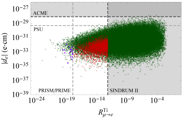
Figure 1: CLFV in the MLRSM for 2 TeV <mWR<<m_{W_{R}}< 30 TeV. The green dots are data points that satisfy only the experimental constraints from the light lepton masses and PMNS matrix. The red dots are data points that also satisfy present bounds from the CLFV, 0​ν​β​β0\nu\beta\beta, EDM’s of charged leptons, and Planck observation. The purple dots are those that satisfy the strongest bounds from future experiments. The shaded regions are regions of parameter space excluded by present experimental bounds. Figures 1a and 1b show that there exist only small chances that τ→μ​γ\tau\to\mu\gamma or τ→e​γ\tau\to e\gamma could be detected in near-future experiments. In figure 1c, the tree-level and 1-loop contributions to μ→e​e​e\mu\to eee are compared, and it shows that we should consider both when calculating BRμ→e​e​e\text{BR}_{\mu\to eee}. Figures 1d−-1f show the linear correlations among various CLFV effects. Note that the strongest future bounds on CLFV come from PRISM/PRIME and PSI, as clearly shown in figure 1e. Figures 1g−-1i show that the μ→e\mu\to e conversion rates for various nuclei have very strong linear correlations with each other. The total number of data points is 83724 (total) = 81132 (green) + 2573 (red) + 19 (purple).
Refer to caption
(a) T1/20​ν|GemaxT_{1/2}^{0\nu}\big|_{\text{Ge}}^{\text{max}} vs. |ην||\eta_{\nu}|
Refer to caption
(b) T1/20​ν|TemaxT_{1/2}^{0\nu}\big|_{\text{Te}}^{\text{max}} vs. |ην||\eta_{\nu}|
Refer to caption
(c) T1/20​ν|XemaxT_{1/2}^{0\nu}\big|_{\text{Xe}}^{\text{max}} vs. |ην||\eta_{\nu}|
Refer to caption
(d) |ην||\eta_{\nu}| vs. |ηNRR||\eta^{R}_{N_{R}}|
Refer to caption
(e) |ην||\eta_{\nu}| vs. |ηδR||\eta_{\delta_{R}}|
Refer to caption
(f) |ηδR||\eta_{\delta_{R}}| vs. |ηNRR||\eta^{R}_{N_{R}}|
Refer to caption
(g) |ηNRL||\eta^{L}_{N_{R}}| vs. |ηNRR||\eta^{R}_{N_{R}}|
Refer to caption
(h) |ηη||\eta_{\eta}| vs. |ηλ||\eta_{\lambda}|
Refer to caption
(i) |ην||\eta_{\nu}| vs. mν1m_{\nu_{1}}
Figure 2: Parameters of 0​ν​β​β0\nu\beta\beta in the MLRSM for 2 TeV <mWR<<m_{W_{R}}< 30 TeV. Figures 2a−-2c show that only cases where ην\eta_{\nu} dominantly determines T1/20​ν|maxT_{1/2}^{0\nu}\big|^{\text{max}} are allowed with a few exceptions by the present and future experimental bounds. Even though the contributions of ηNRR\eta^{R}_{N_{R}} and ηδR\eta_{\delta_{R}} could be comparable to that of ην\eta_{\nu} in principle, such cases have been actually almost excluded by the constraints from CLFV, as shown in figures 2d−-2f. The contributions from ηη\eta_{\eta} or ηλ\eta_{\lambda} are too small compared with experimental bounds, as shown in figure 2h. Figure 2i shows that the present upper bound of the light Majorana neutrino mass from Planck is already below the bounds from KamLAND-Zen and CUORE, which means that 0​ν​β​β0\nu\beta\beta processes are difficult to be detected in near-future experiments since the light neutrino exchange diagrams are dominant for most of the parameter space due to the CLFV constraints.
Refer to caption
(a) |dμ||d_{\mu}| vs. |de||d_{e}|
Refer to caption
(b) |dτ||d_{\tau}| vs. |de||d_{e}|
Refer to caption
(c) |de||d_{e}| vs. Rμ→eTi\text{R}_{\mu\to e}^{\text{Ti}}
Figure 3: EDM’s of charged leptons in the MLRSM for 2 TeV <mWR<<m_{W_{R}}< 30 TeV. The predicted values are found to be too small compared with the present and future bounds, since large EDM’s require small mWRm_{W_{R}} whose regions of parameter space have been largely constrained as shown in figure 4a. Even though the correlations between EDM’s and CLFV are rather weak, as shown in figure 3c, the larger EDM’s generally require the larger CLFV effects since mWRm_{W_{R}} affects both CLFV and EDM’s.
Refer to caption
(a) Rμ→eTi\text{R}_{\mu\to e}^{\text{Ti}} vs. mWRm_{W_{R}}
Refer to caption
(b) Rμ→eTi\text{R}_{\mu\to e}^{\text{Ti}} vs. mN1m_{N_{1}}
Refer to caption
(c) Rμ→eTi\text{R}_{\mu\to e}^{\text{Ti}} vs. mN3m_{N_{3}}
Refer to caption
(d) Rμ→eTi\text{R}_{\mu\to e}^{\text{Ti}} vs. mν1m_{\nu_{1}}
Refer to caption
(e) BRμ→e​γ\text{BR}_{\mu\to e\gamma} vs. mν1m_{\nu_{1}}
Refer to caption
(f) |ην||\eta_{\nu}| vs. ϵ2\epsilon_{2} (≡κ2/κ1)(\equiv\kappa_{2}/\kappa_{1})
Figure 4: Figures 4a−-4e show the effect of CLFV constraints on the masses of neutrinos and the RH gauge boson. Here, Rμ→eTi\text{R}_{\mu\to e}^{\text{Ti}} is chosen since it most clearly divides the colors of data points through its experimental bounds. The smaller values of the lightest light neutrino mass mν1m_{\nu_{1}} produce the larger CLFV effects, as in figures 4d and 4e, since they require the larger values of the heaviest heavy neutrino mass mN3m_{N_{3}} in most of the parameter space, as shown in figure 6f. As a result, the regions of parameter space of small light neutrino masses get constrained by the experimental bounds on CLFV. In figure 4f, additional data points (yellow dots) are also presented in order to show the effects of the perturvativity constraints, and all the data points generated in the ranges of parameters given in table 3 are shown in this plot. For those yellow points, at least one of the coupling constants are larger than 4​π\sqrt{4\pi} while the experimental constraints in the light neutrino sector are still satisfied. This figure shows that ϵ2≡κ2/κ1≲0.01\epsilon_{2}\equiv\kappa_{2}/\kappa_{1}\lesssim 0.01 is satisfied for all the data points due to the perturvativity constraints as well as the condition κ2<10\kappa_{2}<10 GeV, and thus the Higgs mass constraint can be easily satisfied, as mentioned in table 3.
Refer to caption
(a) mWRm_{W_{R}} vs. mN1m_{N_{1}}
Refer to caption
(b) mWRm_{W_{R}} vs. mN1m_{N_{1}}
Refer to caption
(c) mWRm_{W_{R}} vs. mN3m_{N_{3}}
Figure 5: Masses of heavy neutrinos in the TeV-scale MLRSM for 2 TeV <mWR<<m_{W_{R}}< 30 TeV. For figure 5a, the same data set as in the previous plots are used to show the effect of the consraints from CLFV, 0​ν​β​β0\nu\beta\beta, EDM’s, and Planck on the parameter space. The non-perturbative regions are where at least one coupling constant is larger than 4​π\sqrt{4\pi}. Note that green dots in figure 5a do not completely fill the available parameter space because of the constraints on masses and angles in the light lepton sector. For figures 5b and 5c, much more amount of data points was used to show how the present and future bounds constrain the parameter space. Figures 5a and 5b show that the lightest heavy neutrino mass mN1m_{N_{1}} has been notably constrained by the experimental bounds, especially for smaller mWRm_{W_{R}}. Figure 5c is the plot on the heaviest heavy neutrino mass mN3m_{N_{3}}, and it shows that only a small region of parameter space with small mWRm_{W_{R}} seems to have been excluded. Even though these plots in the linear scale are better in presenting the effect of experimental constraints on largest possible masses of heavy neutrinos, they do not correctly show the density distributions since the matrix A(≡f​κ2/2)A~(\equiv f\kappa_{2}/\sqrt{2}) is generated in the logarithmic scale. Plots of mNm_{N} in the logarithmic scale are presented in figure 7. For figures 5b and 5c, the data sets for figures 7b and 7c are used, respectively.
Refer to caption
(a) mWRm_{W_{R}} vs. mN1m_{N_{1}}
Refer to caption
(b) mWRm_{W_{R}} vs. mN3m_{N_{3}}
Refer to caption
(c) mN3m_{N_{3}} vs. mN1m_{N_{1}}
Refer to caption
(d) mWRm_{W_{R}} vs. mν1m_{\nu_{1}}
Refer to caption
(e) mN1m_{N_{1}} vs. mν1m_{\nu_{1}}
Refer to caption
(f) mN3m_{N_{3}} vs. mν1m_{\nu_{1}}
Figure 6: Figures 6a−-6d show the effect of experimental bounds on the masses of neutrinos and the RH gauge boson. Figures 6a and 6b show that the regions with smaller mWRm_{W_{R}} and larger mNm_{N} are more affected by the present bounds on CLFV, 0​ν​β​β0\nu\beta\beta, and EDM’s. Figures 6e and 6f show that, for smaller mν1m_{\nu_{1}}, i.e. for the light neutrino masses with a larger hierarchy, the heavy neutrino masses also generally need to have a larger hierarchy accordingly since MDM_{D} itself does not have the structure that would give hierarchical light neutrino masses. Due to this effect, only larger mWRm_{W_{R}} is generally allowed for smaller mν1m_{\nu_{1}}, as shown in figure 7a, since large mN3m_{N_{3}} requires large vRv_{R}.
Refer to caption
(a) mWRm_{W_{R}} vs. mν1m_{\nu_{1}}
Refer to caption
(b) mWRm_{W_{R}} vs. mN1m_{N_{1}}
Refer to caption
(c) mWRm_{W_{R}} vs. mN3m_{N_{3}}
Refer to caption
(d) mWRm_{W_{R}} vs. mH1+m_{H_{1}^{+}} (≈mδL+⁣+)\big(\approx m_{\delta_{L}^{++}}\big)
Refer to caption
(e) mWRm_{W_{R}} vs. mH2+m_{H_{2}^{+}}
Refer to caption
(f) mWRm_{W_{R}} vs. mδR+⁣+m_{\delta_{R}^{++}}
Figure 7: Masses of neutrinos and charged scalar fields in the MLRSM for mWR<30m_{W_{R}}<30 TeV. The contours of 90 % and 99 % densities are also presented for illustration purposes. According to the 99 % contour in figure 7a, mν1∼0.1m_{\nu_{1}}\sim 0.1 eV for mWR=5m_{W_{R}}=5 TeV and mν1≳6⋅10−3m_{\nu_{1}}\gtrsim 6\cdot 10^{-3} eV for mWR=10m_{W_{R}}=10 TeV. In addition, the 99 % contour in figure 7b shows that mN1≲200m_{N_{1}}\lesssim 200 GeV for mWR<5m_{W_{R}}<5 TeV and mN1≲2m_{N_{1}}\lesssim 2 TeV for mWR<10m_{W_{R}}<10 TeV. While the masses of H1+H_{1}^{+}, δL+⁣+\delta_{L}^{++}, and δR+⁣+\delta_{R}^{++} have been also constrained by the experimental bounds, the mass of H2+H_{2}^{+} which appears only in the Z1Z_{1}-exchange diagrams of CLFV processes has been barely constrained, as shown in figure 7e. Hence, the constraint of mH2+≳10m_{H_{2}^{+}}\gtrsim 10 TeV from the absence of flavour changing neutral current in the quark sector is not considered in this paper. The total number of data points is 51971 = 51561 (red) + 410 (purple).

The most notable result is that the regions of parameter space that allow small light neutrino masses are largely constrained by the experimental bounds from CLFV as well as the constraints from the light neutrino mass and mixing angles. Since the type-I seesaw formula implies det(MνM_{\nu}) ≈\approx det(MDM_{D})2/det(MRM_{R}), we need a hierarchy in the eigenvalues of MDM_{D} or MRM_{R} when light neutrino masses have a hierarchy. However, MDM_{D} is determined from Yukawa couplings and VEV’s, and it generally does not have the appropriate hierarchy in its eigenvalues to give hierachical light neutrino masses for most of the available parameter space. In other words, we generally need a hierarchy in the eigenvalues of MRM_{R}, i.e. in the heavy neutrino masses as well, in order to obtain hierachical light neutrino masses. Since we are considering a range of mNm_{N}, i.e. 0.1 TeV ≲mN≲\lesssim m_{N}\lesssim 100 TeV, the cases of large hierarchies in light neutrino masses are supposed to get constrained accordingly. Furthermore, since the regions of parameter space with large mNm_{N} are largely affected by the experimental constraints from CLFV, small light neutrino masses are disfavored by all those experimental constraints. These results are all clearly presented in several plots in figures 4, 6, and 7. For example, the 99 % contour in figure 7a shows that mν1∼0.1m_{\nu_{1}}\sim 0.1 eV for mWR=5m_{W_{R}}=5 TeV and mν1≳6⋅10−3m_{\nu_{1}}\gtrsim 6\cdot 10^{-3} eV for mWR=10m_{W_{R}}=10 TeV. Note that this does not necessarily mean that there exists a strict lower bound of the light neutrino mass for given mWRm_{W_{R}}, since the results of this paper are based on the naturalness argument such as no fine-tuning in MDM_{D}. Note also that we can observe similar patterns in neutrino mass correlations in any type-I seesaw models, even in the simple extension of the SM only with gauge singlet neutrinos. The difference in the MLRSM, or in a more general class of the left-right symmetric model, is that we can have large CLFV effects and thus the experimental bounds on CLFV are constraining the light neutrino masses. Moreover, since the largest possible hierarchy in heavy neutrino masses is directly associated with mWRm_{W_{R}} and the regions of parameter space with smaller mWRm_{W_{R}} are more constrained by CLFV bounds, we can expect that the discovery of light WRW_{R} as well as any improved experimental bounds on CLFV would largely constrain the regions of parameter space of the normal hierarchy.

Another interesting result is that the mass of the lightest heavy neutrino mN1m_{N_{1}} has been also notably constrained by the present experimental constraints, which is, of course, associated with the result on light neutrino masses just mentioned. This is shown in figures 5a, 5b, 6a, and 7b. For example, the 99 % density contour of figure 7b shows that mN1≲200m_{N_{1}}\lesssim 200 GeV for mWR=5m_{W_{R}}=5 TeV and mN1≲2m_{N_{1}}\lesssim 2 TeV for mWR=10m_{W_{R}}=10 TeV. Due to the mass insertion in the Dirac propagators of heavy neutrinos in some CLFV processes, large heavy neutrino masses generally induce large CLFV effects. Figure 4b explicitly shows how the CLFV bound is constraining mN1m_{N_{1}}. The heaviest heavy neutrino mass is also affected by the experimental bounds, although its effect is rather small, as shown in figures 5c, 6b, and 7c.

While the CLFV effects of muons could be large enough for the associated processes to be detected in near-future experiments, the branching ratios of tau decays are either too small or just around the sensitivities of future experiments, as shown figure 1. The experimental bounds of CLFV are also constraining small masses of charged scalar fields as well as the RH gauge boson, as shown in figure 7. As a result, the 0​ν​β​β0\nu\beta\beta processes through the heavy neutrinos as well as RH gauge boson (denoted by ηNRR\eta^{R}_{N_{R}}) and also processes through δR+⁣+\delta_{R}^{++} as well as the RH gauge boson (denoted by ηδR\eta_{\delta_{R}}) are both suppressed. Hence, for most data points that satisfy the present experimental constraints, the dominant contribution to 0​ν​β​β0\nu\beta\beta comes from the process of the light neutrino exchange (denoted by ην\eta_{\nu}), as shown in figures 2a−-2c. However, since the upper bound of the light neutrino mass by Planck is already below the bounds of future experiments as shown in figure 2i, i.e. the light neutrino exchange channel has been largely constrained by the Planck observation, the possibility to detect 0​ν​β​β0\nu\beta\beta processes in near-future experiments is small. As for the EDM’s of electrons, there seems to be also only small chances that they could be detected in near-future experiments as shown in figure 3, since the largest possible EDM’s of electrons are well below the future sensitivities of the planned experiement. In addition, the EDM’s of muons and taus are too small compared with the present upper bounds. Note that the EDM’s of charged leptons has been also constrained by the experimental bounds from CLFV, since large EDM’s generally require small mWRm_{W_{R}} and large mNm_{N} and such regions of parameter space are largely affected by those experimental constraints. Note also that, even with the relatively small values of the RH scale, i.e. vR<65v_{R}<65 TeV corresponding to mWR<30m_{W_{R}}<30 TeV, the observables of CLFV, 0​ν​β​β0\nu\beta\beta, and EDM’s cover very wide ranges, e.g. roughly 10−20≲BRμ→e​γ≲10−310^{-20}\lesssim\text{BR}_{\mu\to e\gamma}\lesssim 10^{-3} and 10−35​e⋅cm≲|de|≲10−29​e⋅cm10^{-35}~e\cdot\text{cm}\lesssim|d_{e}|\lesssim 10^{-29}~e\cdot\text{cm}. Hence, neither a success nor a failure in detecting one of these effects rules out even the TeV-scale MLRSM, unless any other experimental results are simultaneously considered.

5 Conclusion

In this paper, the procedure to construct lepton mass matrices is presented in the MLRSM of type-I dominance with the parity symmetry, and the conditions for the TeV-scale MLRSM without fine-tuning are also discussed, i.e. either (i) κ1≫κ2\kappa_{1}\gg\kappa_{2} and fi​j≪f~i​jf_{ij}\ll\tilde{f}_{ij}, which implies VLℓ≈VRℓV^{\ell}_{L}\approx V^{\ell}_{R}, or (ii) κ1≪κ2\kappa_{1}\ll\kappa_{2} and fi​j≫f~i​jf_{ij}\gg\tilde{f}_{ij}, which implies VLℓ≈VRℓ​e−i​αV^{\ell}_{L}\approx V^{\ell}_{R}e^{-i\alpha}. Based on these results, the phenomenology of the TeV-scale MLRSM is numerically investigated when the masses of light neutrinos are in the normal hierarchy, and the numerical results on how the present and future experimental bounds from the CLFV, 0​ν​β​β0\nu\beta\beta, EDM’s of charged leptons, and Planck observation constrain the parameter space of the MLRSM are presented.

According to the numerical results, the regions of parameter space of small light neutrino masses have been constrained by the experimental bounds on CLFV effects, although it does not necessarily mean there exists a strict lower bound of light neutrino masses. The lightest heavy neutrino mass is also found to have been notably constrained by the present experimental bounds especially for small mWRm_{W_{R}}. In addition, it has been shown that all the 0​ν​β​β0\nu\beta\beta processes and the EDM’s of charged leptons have been suppressed by the experimental constraints from CLFV, and we have at best only small chances to detect any of these effects in near-future experiments.

Note that the results of this paper are based on several nontrivial assumptions such as (i) type-I seesaw dominance, (ii) the parity symmetry, and (iii) the normal hierarchy in light neutrino masses. Furthermore, it should be emphasized that this paper is considering the TeV-scale phenomenology of the MLRSM without fine-tuning of model parameters. If fine-tuning is allowed, significantly different predictions could be made.

Acknowledgement

The author would like to thank Dr. R.N. Mohapatra for valuable discussions and encouragement. This work is supported by the National Science Foundation grant NSF-PHY-1620074.

Appendix A Expressions of observables

In this paper, the expressions presented in reference [10] are mostly used. The exceptions are the form factors FRZ1F^{Z_{1}}_{R} and BR​Rμ​e​e​eB_{RR}^{\mu eee}: for FRZ1F^{Z_{1}}_{R}, a mixed expression from references [10] and [32] is used; for BR​Rμ​e​e​eB_{RR}^{\mu eee}, the suppression factor (mWL/mWR)2(m_{W_{L}}/m_{W_{R}})^{2} is multiplied to the whole expression. The normalized Yukawa couplings h~L\tilde{h}_{L} and h~R\tilde{h}_{R} are explicitly distinguished in this paper, since they are generally different even with the manifest left-right symmetry.

A.1 Charged lepton flavour violation

The normalized Yukawa couplings h~L\tilde{h}_{L}, h~R\tilde{h}_{R} in the charged lepton mass basis are given by [33]

h~L\displaystyle\tilde{h}_{L} ≡2g​VLℓ​𝖳​hL​VLℓ=2g​VLℓ​𝖳​ML∗​e−i​θL2​vL​VLℓ,\displaystyle\equiv\frac{2}{g}V_{L}^{\ell\mathsf{T}}h_{L}V_{L}^{\ell}=\frac{2}{g}V_{L}^{\ell\mathsf{T}}\frac{M_{L}^{*}e^{-i\theta_{L}}}{\sqrt{2}v_{L}}V_{L}^{\ell}, (114)
h~R\displaystyle\tilde{h}_{R} ≡2g​VRℓ​𝖳​hR​VRℓ=2g​VRℓ​𝖳​MR2​vR​VRℓ=VRℓ​𝖳​MRmWR​VRℓ.\displaystyle\equiv\frac{2}{g}V_{R}^{\ell\mathsf{T}}h_{R}V_{R}^{\ell}=\frac{2}{g}V_{R}^{\ell\mathsf{T}}\frac{M_{R}}{\sqrt{2}v_{R}}V_{R}^{\ell}=V_{R}^{\ell\mathsf{T}}\frac{M_{R}}{m_{W_{R}}}V_{R}^{\ell}. (115)

Note that h~L≠h~R\tilde{h}_{L}\neq\tilde{h}_{R} in general since VLℓ≠VRℓV_{L}^{\ell}\neq V_{R}^{\ell} for nonzero α\alpha, although h≡hL=hRh\equiv h_{L}=h_{R} with the parity symmetry. The loop functions of CLFV are given in appendix A.1.4.

A.1.1 ℓa→ℓb​γ\ell_{a}\to\ell_{b}\gamma

For on-shell decay ℓa→ℓb​γ\ell_{a}\to\ell_{b}\gamma, the branching ratio is given by

BRℓa→ℓb​γ=αW3​sW2​mℓa5256​π2​mWL4​Γℓa​(|GLγ|2+|GRγ|2)\displaystyle\text{BR}_{\ell_{a}\to\ell_{b}\gamma}=\frac{\alpha_{W}^{3}s_{W}^{2}m_{\ell_{a}}^{5}}{256\pi^{2}m_{W_{L}}^{4}\Gamma_{\ell_{a}}}\big(|G_{L}^{\gamma}|^{2}+|G_{R}^{\gamma}|^{2}\big) (116)

where αW≡g2/(4​π)\alpha_{W}\equiv g^{2}/(4\pi), sW≡sin⁡θWs_{W}\equiv\sin{\theta_{W}}, and Γℓa\Gamma_{\ell_{a}} is the decay rates of ℓa\ell_{a}: Γμ=2.996⋅10−19\Gamma_{\mu}=2.996\cdot 10^{-19} GeV and Γτ=2.267⋅10−12\Gamma_{\tau}=2.267\cdot 10^{-12} GeV [34]. The form factors GLγG_{L}^{\gamma}, GRγG_{R}^{\gamma} are given by

GLγ\displaystyle G_{L}^{\gamma} =∑i=13[Vμ​i​Ve​i∗​ξ2​G1γ​(xi)−Sμ​i∗​Ve​i∗​ξ​e−i​α​G2γ​(xi)​mNimℓa+Vμ​i​Ve​i∗​mWL2mWR2​G1γ​(yi)+h~R​μ​i​h~R​e​i∗​23​mWL2mδR+⁣+2],\displaystyle=\sum_{i=1}^{3}\bigg[V_{\mu i}V_{ei}^{*}\xi^{2}G_{1}^{\gamma}(x_{i})-S_{\mu i}^{*}V_{ei}^{*}\xi e^{-i\alpha}G_{2}^{\gamma}(x_{i})\frac{m_{N_{i}}}{m_{\ell_{a}}}+V_{\mu i}V_{ei}^{*}\frac{m_{W_{L}}^{2}}{m_{W_{R}}^{2}}G_{1}^{\gamma}(y_{i})+\tilde{h}_{R\mu i}\tilde{h}_{Rei}^{*}\frac{2}{3}\frac{m_{W_{L}}^{2}}{m_{\delta_{R}^{++}}^{2}}\bigg], (117)
GRγ\displaystyle G_{R}^{\gamma} =∑i=13[Sμ​i∗​Se​i​G1γ​(xi)−Vμ​i​Se​i​ξ​ei​α​G2γ​(xi)​mNimℓa+h~L​μ​i​h~L​e​i∗​(23​mWL2mδL+⁣+2+112​mWL2mH1+2)]\displaystyle=\sum_{i=1}^{3}\bigg[S_{\mu i}^{*}S_{ei}G_{1}^{\gamma}(x_{i})-V_{\mu i}S_{ei}\xi e^{i\alpha}G_{2}^{\gamma}(x_{i})\frac{m_{N_{i}}}{m_{\ell_{a}}}+\tilde{h}_{L\mu i}\tilde{h}_{Lei}^{*}\bigg(\frac{2}{3}\frac{m_{W_{L}}^{2}}{m_{\delta_{L}^{++}}^{2}}+\frac{1}{12}\frac{m_{W_{L}}^{2}}{m_{H_{1}^{+}}^{2}}\bigg)\bigg] (118)

where xi=(mNi/mWL)2x_{i}=(m_{N_{i}}/m_{W_{L}})^{2} and yi=(mNi/mWR)2y_{i}=(m_{N_{i}}/m_{W_{R}})^{2}. The initial and final charged leptons have opposite chiralities, and LL or RR in GL,RγG_{L,R}^{\gamma} denotes the chirality of the initial charged lepton. The Feynman diagrams of on-shell μ→e​γ\mu\to e\gamma are given in figure 8.

(a) GLγG_{L}^{\gamma}
(b) GLγG_{L}^{\gamma}
(c) GLγG_{L}^{\gamma}
(d) GLγG_{L}^{\gamma}
(e) GLγG_{L}^{\gamma}
(f) GRγG_{R}^{\gamma}
(g) GRγG_{R}^{\gamma}
(h) GRγG_{R}^{\gamma}
(i) GRγG_{R}^{\gamma}
Figure 8: Feynman diagrams of on-shell μ→e​γ\mu\to e\gamma. Here, WL+≈W1++ξ​e−i​α​W2+W_{L}^{+}\approx W_{1}^{+}+\xi e^{-i\alpha}W_{2}^{+} and WR+≈−ξ​ei​α​W1++W2+W_{R}^{+}\approx-\xi e^{i\alpha}W_{1}^{+}+W_{2}^{+}. Figures 8a−-8e contribute to GLγG_{L}^{\gamma}, and figures 8f−-8i to GRγG_{R}^{\gamma}. The arrows in neutrino propagators denote the directions of the propagation of Ni=NR​i+NR​icN_{i}=N_{Ri}+N_{Ri}^{c}.

A.1.2 μ→e​e​e\mu\to eee

The tree-level contribution to μ→e​e​e\mu\to eee is

BRμ→e​e​etree=αW4​mμ524576​π3​mWL4​Γμ​(4​π)22​αW2​(|h~L​μ​e​h~L​e​e∗|2​mWL4mδL+⁣+4+|h~R​μ​e​h~R​e​e∗|2​mWL4mδR+⁣+4).\displaystyle\text{BR}_{\mu\to eee}^{\text{tree}}=\frac{\alpha_{W}^{4}m_{\mu}^{5}}{24576\pi^{3}m_{W_{L}}^{4}\Gamma_{\mu}}\frac{(4\pi)^{2}}{2\alpha_{W}^{2}}\left(\big|\tilde{h}_{L\mu e}\tilde{h}_{Lee}^{*}\big|^{2}\frac{m_{W_{L}}^{4}}{m_{\delta_{L}^{++}}^{4}}+\big|\tilde{h}_{R\mu e}\tilde{h}_{Ree}^{*}\big|^{2}\frac{m_{W_{L}}^{4}}{m_{\delta_{R}^{++}}^{4}}\right). (119)

The Feynman diagrams of the tree-level processes are given in figure 9.

(a)
(b)
Figure 9: Feynman diagrams of the tree-level processes of μ→e​e​e\mu\to eee.

The one-loop type-I seesaw contribution is given by [35, 36]

BRμ→e​e​etype-I\displaystyle\text{BR}_{\mu\to eee}^{\text{type-I}} =αW4​mμ524576​π3​mWL4​Γμ[2{|12BL​Lμ​e​e​e+FLZ1−2sW2(FLZ1−FLγ)|2+|12BR​Rμ​e​e​e−2sW2(FRZ1−FRγ)|2}\displaystyle=\frac{\alpha_{W}^{4}m_{\mu}^{5}}{24576\pi^{3}m_{W_{L}}^{4}\Gamma_{\mu}}\bigg[2\bigg\{\bigg|\frac{1}{2}B_{LL}^{\mu eee}+F_{L}^{Z_{1}}-2s_{W}^{2}\big(F_{L}^{Z_{1}}-F_{L}^{\gamma}\big)\bigg|^{2}+\bigg|\frac{1}{2}B_{RR}^{\mu eee}-2s_{W}^{2}\big(F_{R}^{Z_{1}}-F_{R}^{\gamma}\big)\bigg|^{2}\bigg\}
+|2​sW2​(FLZ1−FLγ)−BL​Rμ​e​e​e|2+|2​sW2​(FRZ1−FRγ)−(FRZ1+BR​Lμ​e​e​e)|2\displaystyle\qquad\qquad+\bigg|2s_{W}^{2}\big(F_{L}^{Z_{1}}-F_{L}^{\gamma}\big)-B_{LR}^{\mu eee}\bigg|^{2}+\bigg|2s_{W}^{2}\big(F_{R}^{Z_{1}}-F_{R}^{\gamma}\big)-\big(F_{R}^{Z_{1}}+B_{RL}^{\mu eee}\big)\bigg|^{2}
+8sW2{Re[(2FLZ1+BL​Lμ​e​e​e+BL​Rμ​e​e​e)GRγ∗]+Re[(FRZ1+BR​Rμ​e​e​e+BR​Lμ​e​e​e)GLγ∗]}\displaystyle\qquad\qquad+8s_{W}^{2}\bigg\{\text{Re}\bigg[\big(2F_{L}^{Z_{1}}+B_{LL}^{\mu eee}+B_{LR}^{\mu eee}\big)G_{R}^{\gamma*}\bigg]+\text{Re}\bigg[\big(F_{R}^{Z_{1}}+B_{RR}^{\mu eee}+B_{RL}^{\mu eee}\big)G_{L}^{\gamma*}\bigg]\bigg\}
−48sW4{Re[(FLZ1−FLγ)GRγ∗]+Re[(FRZ1−FRγ)GLγ∗]}\displaystyle\qquad\qquad-48s_{W}^{4}\bigg\{\text{Re}\bigg[\big(F_{L}^{Z_{1}}-F_{L}^{\gamma}\big)G_{R}^{\gamma*}\bigg]+\text{Re}\bigg[\big(F_{R}^{Z_{1}}-F_{R}^{\gamma}\big)G_{L}^{\gamma*}\bigg]\bigg\}
+32sW4(|GLγ|2+|GRγ|2){ln(mμ2me2)−114}],\displaystyle\qquad\qquad+32s_{W}^{4}\big(|G_{L}^{\gamma}|^{2}+|G_{R}^{\gamma}|^{2}\big)\bigg\{\ln{\bigg(\frac{m_{\mu}^{2}}{m_{e}^{2}}\bigg)}-\frac{11}{4}\bigg\}\bigg], (120)

and the interference terms are

BRμ→e​e​etree+type-I\displaystyle\text{BR}_{\mu\to eee}^{\text{tree+type-I}} =αW4​mμ524576​π3​mWL4​Γμ2​(4​π)αW×\displaystyle=\frac{\alpha_{W}^{4}m_{\mu}^{5}}{24576\pi^{3}m_{W_{L}}^{4}\Gamma_{\mu}}\frac{2(4\pi)}{\alpha_{W}}\times
[mWL2mδL+⁣+2Re[h~L​μ​e∗h~L​e​e{2sW2FLγ+4sW2GRγ+BL​Lμ​e​e​e+FLZ1(1−2sW2)}]\displaystyle\qquad\bigg[\frac{m_{W_{L}}^{2}}{m_{\delta_{L}^{++}}^{2}}\text{Re}\bigg[\tilde{h}_{L\mu e}^{*}\tilde{h}_{Lee}\bigg\{2s_{W}^{2}F_{L}^{\gamma}+4s_{W}^{2}G_{R}^{\gamma}+B_{LL}^{\mu eee}+F_{L}^{Z_{1}}(1-2s_{W}^{2})\bigg\}\bigg]
+mWL2mδR+⁣+2Re[h~R​μ​e∗h~R​e​e{2sW2FRγ+4sW2GLγ+BR​Rμ​e​e​e−2sW2FRZ1}]].\displaystyle\qquad\qquad+\frac{m_{W_{L}}^{2}}{m_{\delta_{R}^{++}}^{2}}\text{Re}\bigg[\tilde{h}_{R\mu e}^{*}\tilde{h}_{Ree}\bigg\{2s_{W}^{2}F_{R}^{\gamma}+4s_{W}^{2}G_{L}^{\gamma}+B_{RR}^{\mu eee}-2s_{W}^{2}F_{R}^{Z_{1}}\bigg\}\bigg]\bigg]. (121)

The form factors for the off-shell photon exchange are

FLγ\displaystyle F_{L}^{\gamma} =∑i=13[Sμ​i∗​Se​i​Fγ​(xi)−h~L​μ​i​h~L​e​i∗​(23​mWL2mδL+⁣+​ln⁡mμ2mδL+⁣++118​mWL2mH1+)],\displaystyle=\sum_{i=1}^{3}\left[S_{\mu i}^{*}S_{ei}F_{\gamma}(x_{i})-\tilde{h}_{L\mu i}\tilde{h}_{Lei}^{*}\bigg(\frac{2}{3}\frac{m_{W_{L}}^{2}}{m_{\delta_{L}^{++}}}\ln{\frac{m_{\mu}^{2}}{m_{\delta_{L}^{++}}}}+\frac{1}{18}\frac{m_{W_{L}}^{2}}{m_{H_{1}^{+}}}\bigg)\right], (122)
FRγ\displaystyle F_{R}^{\gamma} =∑i=13[Vμ​i​Ve​i∗​(ξ2​Fγ​(xi)+mWL2mWR2​Fγ​(yi))−h~R​μ​i​h~R​e​i∗​23​mWL2mδR+⁣+​ln⁡mμ2mδR+⁣+].\displaystyle=\sum_{i=1}^{3}\left[V_{\mu i}V_{ei}^{*}\bigg(\xi^{2}F_{\gamma}(x_{i})+\frac{m_{W_{L}}^{2}}{m_{W_{R}}^{2}}F_{\gamma}(y_{i})\bigg)-\tilde{h}_{R\mu i}\tilde{h}_{Rei}^{*}\frac{2}{3}\frac{m_{W_{L}}^{2}}{m_{\delta_{R}^{++}}}\ln{\frac{m_{\mu}^{2}}{m_{\delta_{R}^{++}}}}\right]. (123)

For the Z1Z_{1}-exchange diagrams, the form factors are given by

FLZ1\displaystyle F_{L}^{Z_{1}} =∑i,j=13Sμ​i∗Se​j[δi​j{FZ(xi)+2GZ(0,xi)}\displaystyle=\sum_{i,j=1}^{3}S_{\mu i}^{*}S_{ej}\bigg[\delta_{ij}\big\{F_{Z}(x_{i})+2G_{Z}(0,x_{i})\big\}
+(S𝖳S∗)i​j{GZ(xi,xj)−GZ(0,xi)−GZ(0,xj)}+(S†S)i​jHZ(xi,xj)],\displaystyle\qquad\qquad+(S^{\mathsf{T}}S^{*})_{ij}\big\{G_{Z}(x_{i},x_{j})-G_{Z}(0,x_{i})-G_{Z}(0,x_{j})\big\}+(S^{\dagger}S)_{ij}H_{Z}(x_{i},x_{j})\bigg], (124)
FRZ1\displaystyle F_{R}^{Z_{1}} =∑i=13Vμ​iVe​i∗[8​ζ3​cW21−2​sW2{FZ(yi)+2GZ(0,yi)−yi2}+2(κ1​κ2vEW​vR)2DZ(yi,xi)\displaystyle=\sum_{i=1}^{3}V_{\mu i}V_{ei}^{*}\bigg[\frac{8\zeta_{3}c_{W}^{2}}{\sqrt{1-2s_{W}^{2}}}\bigg\{F_{Z}(y_{i})+2G_{Z}(0,y_{i})-\frac{y_{i}}{2}\bigg\}+2\left(\frac{\kappa_{1}\kappa_{2}}{v_{\text{EW}}v_{R}}\right)^{2}D_{Z}(y_{i},x_{i})
+(κ12−κ222​vEW​vR)2DZ(yi,zi)]\displaystyle\qquad\qquad+\left(\frac{\kappa_{1}^{2}-\kappa_{2}^{2}}{\sqrt{2}v_{\text{EW}}v_{R}}\right)^{2}D_{Z}(y_{i},z_{i})\bigg] (125)

where zi=(mNi/mH2+)2z_{i}=(m_{N_{i}}/m_{H_{2}^{+}})^{2}, cW≡cos⁡θWc_{W}\equiv\cos{\theta_{W}}, and ζ3\zeta_{3} is the Z1Z_{1}-Z2Z_{2} mixing parameter given by equation 53. The Feynman diagrams that contribute to FL,RγF_{L,R}^{\gamma} and FL,RZ1F_{L,R}^{Z_{1}} are presented in reference [33]. The form factors of the box diagrams are written as

BL​Lμ​e​e​e\displaystyle B_{LL}^{\mu eee} =−2∑i=13Sμ​i∗Se​i[FXbox(0,xi)−FXbox(0,0)]\displaystyle=-2\sum_{i=1}^{3}S_{\mu i}^{*}S_{ei}\big[F_{\text{Xbox}}(0,x_{i})-F_{\text{Xbox}}(0,0)\big]
+∑i,j=13Sμ​i∗Se​j[−2Se​j∗Se​i{FXbox(xi,xj)−FXbox(0,xj)−FXbox(0,xi)+FXbox(0,0)}\displaystyle\qquad+\sum_{i,j=1}^{3}S_{\mu i}^{*}S_{ej}\bigg[-2S_{ej}^{*}S_{ei}\big\{F_{\text{Xbox}}(x_{i},x_{j})-F_{\text{Xbox}}(0,x_{j})-F_{\text{Xbox}}(0,x_{i})+F_{\text{Xbox}}(0,0)\big\}
+Se​i∗Se​jGbox(xi,xj,1)],\displaystyle\qquad\qquad+S_{ei}^{*}S_{ej}G_{\text{box}}(x_{i},x_{j},1)\bigg], (126)
BR​Rμ​e​e​e\displaystyle B_{RR}^{\mu eee} =−2mWL2mWR2∑i,j=13Vμ​iVe​i∗[FXbox(0,yi)−FXbox(0,0)]\displaystyle=-2\frac{m_{W_{L}}^{2}}{m_{W_{R}}^{2}}\sum_{i,j=1}^{3}V_{\mu i}V_{ei}^{*}\big[F_{\text{Xbox}}(0,y_{i})-F_{\text{Xbox}}(0,0)\big]
+mWL2mWR2∑i,j=13Vμ​iVe​j∗[−2Ve​jVe​i∗{FXbox(yi,yj)−FXbox(0,yj)−FXbox(0,yi)+FXbox(0,0)}\displaystyle\qquad+\frac{m_{W_{L}}^{2}}{m_{W_{R}}^{2}}\sum_{i,j=1}^{3}V_{\mu i}V_{ej}^{*}\bigg[-2V_{ej}V_{ei}^{*}\big\{F_{\text{Xbox}}(y_{i},y_{j})-F_{\text{Xbox}}(0,y_{j})-F_{\text{Xbox}}(0,y_{i})+F_{\text{Xbox}}(0,0)\big\}
+Ve​iVe​j∗Gbox(yi,yj,1)],\displaystyle\qquad\qquad+V_{ei}V_{ej}^{*}G_{\text{box}}(y_{i},y_{j},1)\bigg], (127)
BL​Rμ​e​e​e\displaystyle B_{LR}^{\mu eee} =12​mWL2mWR2​∑i,j=13Sμ​i∗​Se​j​Ve​i​Ve​j∗​Gbox​(xi,xj,mWL2mWR2),\displaystyle=\frac{1}{2}\frac{m_{W_{L}}^{2}}{m_{W_{R}}^{2}}\sum_{i,j=1}^{3}S_{\mu i}^{*}S_{ej}V_{ei}V_{ej}^{*}G_{\text{box}}\bigg(x_{i},x_{j},\frac{m_{W_{L}}^{2}}{m_{W_{R}}^{2}}\bigg), (128)
BR​Lμ​e​e​e\displaystyle B_{RL}^{\mu eee} =12​mWL2mWR2​∑i,j=13Vμ​i​Ve​j∗​Se​i∗​Se​j​Gbox​(xi,xj,mWL2mWR2).\displaystyle=\frac{1}{2}\frac{m_{W_{L}}^{2}}{m_{W_{R}}^{2}}\sum_{i,j=1}^{3}V_{\mu i}V_{ej}^{*}S_{ei}^{*}S_{ej}G_{\text{box}}\bigg(x_{i},x_{j},\frac{m_{W_{L}}^{2}}{m_{W_{R}}^{2}}\bigg). (129)

Here, the masses of light neutrinos and the momenta of external fields are assumed to be zero. The Feynman diagrams of the box diagrams are presented in figure 10.

(a) BL​Lμ​e​e​eB_{LL}^{\mu eee}
(b) BL​Lμ​e​e​eB_{LL}^{\mu eee}
(c) BR​Rμ​e​e​eB_{RR}^{\mu eee}
(d) BR​Rμ​e​e​eB_{RR}^{\mu eee}
(e) BL​Rμ​e​e​eB_{LR}^{\mu eee}
(f) BR​Lμ​e​e​eB_{RL}^{\mu eee}
Figure 10: Feynman diagrams of Bμ​e​e​eB^{\mu eee}. Note that the arrows in neutrino propagators indicate the directions of the propagation of νi=νL​i+νL​ic\nu_{i}=\nu_{Li}+\nu_{Li}^{c} or Ni=NR​i+NR​icN_{i}=N_{Ri}+N_{Ri}^{c}.

A.1.3 μ→e\mu\to e

The μ→e\mu\to e conversion rate is given by [33, 37, 38, 36]

Rμ→eA⁡(N,Z)=αem3​αW4​mμ516​π2​mWL4​Γcapt​Zeff4Z​|Fp​(−mμ2)|2​(|QLW|2+|QRW|2).\displaystyle\text{R}_{\mu\to e}^{A(N,Z)}=\frac{\alpha_{\text{em}}^{3}\alpha_{W}^{4}m_{\mu}^{5}}{16\pi^{2}m_{W_{L}}^{4}\Gamma_{\text{capt}}}\frac{Z_{\text{eff}}^{4}}{Z}\big|F_{p}(-m_{\mu}^{2})\big|^{2}\big(\big|Q_{L}^{W}\big|^{2}+\big|Q_{R}^{W}\big|^{2}\big). (130)

Here, AA, NN, and ZZ are the mass, neutron, and atomic numbers of a nucleus, respectively, and ZeffZ_{\text{eff}} is the effective atomic number. The parameter FpF_{p} is the nuclear form factor, Γcapt\Gamma_{\text{capt}} is the capture rate, and αem≡e2/(4​π)\alpha_{\text{em}}\equiv e^{2}/(4\pi). The values of FpF_{p} and Γcapt\Gamma_{\text{capt}} of various nuclei are summarized in table 6 [38].

Nucleus NZA{}^{A}_{Z}\text{N} ZeffZ_{\text{eff}} |Fp​(−mμ2)||F_{p}(-m_{\mu}^{2})| Γcapt​(106​s−1)\Gamma_{\text{capt}}~(10^{6}~s^{-1})
Al1327{}^{27}_{13}\text{Al} 11.5 0.64 0.7054
Ti2248{}^{48}_{22}\text{Ti} 17.6 0.54 2.59
Au79197{}^{197}_{79}\text{Au} 33.5 0.16 13.07
Pb82208{}^{208}_{82}\text{Pb} 34.0 0.15 13.45
Table 6: Form factors and capture rates of various nuclei associated with μ→e\mu\to e conversion.

The form factors in equation 130 are given by

QL,RW=(2​Z+N)​[WL,Ru−23​sW2​GR,Lγ]+(Z+2​N)​[WL,Rd+13​sW2​GR,Lγ]\displaystyle Q_{L,R}^{W}=(2Z+N)\bigg[W_{L,R}^{u}-\frac{2}{3}s_{W}^{2}G_{R,L}^{\gamma}\bigg]+(Z+2N)\bigg[W_{L,R}^{d}+\frac{1}{3}s_{W}^{2}G_{R,L}^{\gamma}\bigg] (131)

and

WL,Ru\displaystyle W_{L,R}^{u} =23​sW2​FL,Rγ+(−14+23​sW2)​FL,RZ1+14​(BL​L,R​Rμ​e​u​u+BL​R,R​Lμ​e​u​u),\displaystyle=\frac{2}{3}s_{W}^{2}F_{L,R}^{\gamma}+\bigg(-\frac{1}{4}+\frac{2}{3}s_{W}^{2}\bigg)F_{L,R}^{Z_{1}}+\frac{1}{4}\bigg(B_{LL,RR}^{\mu euu}+B_{LR,RL}^{\mu euu}\bigg), (132)
WL,Rd\displaystyle W_{L,R}^{d} =−13​sW2​FL,Rγ+(14−13​sW2)​FL,RZ1+14​(BL​L,R​Rμ​e​d​d+BL​R,R​Lμ​e​d​d).\displaystyle=-\frac{1}{3}s_{W}^{2}F_{L,R}^{\gamma}+\bigg(\frac{1}{4}-\frac{1}{3}s_{W}^{2}\bigg)F_{L,R}^{Z_{1}}+\frac{1}{4}\bigg(B_{LL,RR}^{\mu edd}+B_{LR,RL}^{\mu edd}\bigg). (133)

The box diagram form factors are

BL​Lμ​e​u​u\displaystyle B_{LL}^{\mu euu} =∑i=13Sμ​i∗​Se​i​[Fbox​(0,xi)−Fbox​(0,0)],\displaystyle=\sum_{i=1}^{3}S_{\mu i}^{*}S_{ei}[F_{\text{box}}(0,x_{i})-F_{\text{box}}(0,0)], (134)
BL​Lμ​e​d​d\displaystyle B_{LL}^{\mu edd} =∑i=13Sμ​i∗Se​i[FXbox(0,xi)−FXbox(0,0)\displaystyle=\sum_{i=1}^{3}S_{\mu i}^{*}S_{ei}\big[F_{\text{Xbox}}(0,x_{i})-F_{\text{Xbox}}(0,0)
+|VL​t​dq|2{FXbox(xt,xi)−FXbox(0,xi)−FXbox(0,xt)+FXbox(0,0)}],\displaystyle\qquad\qquad+|V_{Ltd}^{q}|^{2}\{F_{\text{Xbox}}(x_{t},x_{i})-F_{\text{Xbox}}(0,x_{i})-F_{\text{Xbox}}(0,x_{t})+F_{\text{Xbox}}(0,0)\}\big], (135)
BR​Rμ​e​u​u\displaystyle B_{RR}^{\mu euu} =∑i=13Vμ​i​Ve​i∗​[Fbox​(0,xi)−Fbox​(0,0)],\displaystyle=\sum_{i=1}^{3}V_{\mu i}V_{ei}^{*}[F_{\text{box}}(0,x_{i})-F_{\text{box}}(0,0)], (136)
BR​Rμ​e​d​d\displaystyle B_{RR}^{\mu edd} =∑i=13Vμ​iVe​i∗[FXbox(0,xi)−FXbox(0,0)\displaystyle=\sum_{i=1}^{3}V_{\mu i}V_{ei}^{*}\big[F_{\text{Xbox}}(0,x_{i})-F_{\text{Xbox}}(0,0)
+|VR​t​dq|2{FXbox(xt,xi)−FXbox(0,xi)−FXbox(0,xt)+FXbox(0,0)}],\displaystyle\qquad\qquad+|V_{Rtd}^{q}|^{2}\{F_{\text{Xbox}}(x_{t},x_{i})-F_{\text{Xbox}}(0,x_{i})-F_{\text{Xbox}}(0,x_{t})+F_{\text{Xbox}}(0,0)\}\big], (137)

and BL​Rμ​e​q​q=BR​Lμ​e​q​q=0B_{LR}^{\mu eqq}=B_{RL}^{\mu eqq}=0 due to their chiral structures. Here, xt=mt2/mWL2x_{t}=m_{t}^{2}/m_{W_{L}}^{2} and yt=mt2/mWR2y_{t}=m_{t}^{2}/m_{W_{R}}^{2} where mtm_{t} is the mass of a top quark, and the masses of all the other quarks as well as light neutrinos are assumed to be zero. The matrix VLqV_{L}^{q} is the Cabibbo-Kobayashi-Maskawa matrix, and VRqV_{R}^{q} is its RH counterpart. Note that VLq≠VRqV_{L}^{q}\neq V_{R}^{q} for nonzero α\alpha, although VL​t​dq=VR​t​dqV_{Ltd}^{q}=V_{Rtd}^{q} is assumed for the numerical analysis in this paper. The momenta of external fields are also assumed to be zero. The Feynman diagrams of the box diagrams are given in figure 11.

(a) BL​Lμ​e​u​uB_{LL}^{\mu euu}
(b) BL​Lμ​e​d​dB_{LL}^{\mu edd}
(c) BR​Rμ​e​u​uB_{RR}^{\mu euu}
(d) BR​Rμ​e​d​dB_{RR}^{\mu edd}
Figure 11: Feynman diagrams of Bμ​e​q​qB^{\mu eqq}.

A.1.4 Loop functions

The loop functions of CLFV are

Fγ​(x)\displaystyle F_{\gamma}(x) =7​x3−x2−12​x12​(1−x)3−x4−10​x3+12​x26​(1−x)4​ln⁡x,\displaystyle=\frac{7x^{3}-x^{2}-12x}{12(1-x)^{3}}-\frac{x^{4}-10x^{3}+12x^{2}}{6(1-x)^{4}}\ln{x}, (138)
G1γ​(x)\displaystyle G^{\gamma}_{1}(x) =−2​x3+5​x2−x4​(1−x)3−3​x32​(1−x)4​ln⁡x,\displaystyle=-\frac{2x^{3}+5x^{2}-x}{4(1-x)^{3}}-\frac{3x^{3}}{2(1-x)^{4}}\ln{x}, (139)
G2γ​(x)\displaystyle G^{\gamma}_{2}(x) =x2−11​x+42​(1−x)2−3​x2(1−x)3​ln⁡x,\displaystyle=\frac{x^{2}-11x+4}{2(1-x)^{2}}-\frac{3x^{2}}{(1-x)^{3}}\ln{x}, (140)
FZ​(x)\displaystyle F_{Z}(x) =−5​x2​(1−x)−5​x22​(1−x)2​ln⁡x,\displaystyle=-\frac{5x}{2(1-x)}-\frac{5x^{2}}{2(1-x)^{2}}\ln{x}, (141)
GZ​(x,y)\displaystyle G_{Z}(x,y) =−12​(1−x)​[x2​(1−y)1−x​ln⁡x−y2​(1−x)1−y​ln⁡y],\displaystyle=-\frac{1}{2(1-x)}\left[\frac{x^{2}(1-y)}{1-x}\ln{x}-\frac{y^{2}(1-x)}{1-y}\ln{y}\right], (142)
HZ​(x,y)\displaystyle H_{Z}(x,y) =x​y4​(x−y)​[x⁡(x−4)1−x​ln⁡x−y⁡(y−4)1−y​ln⁡y],\displaystyle=\frac{\sqrt{xy}}{4(x-y)}\left[\frac{x(x-4)}{1-x}\ln{x}-\frac{y(y-4)}{1-y}\ln{y}\right], (143)
DZ​(x,y)\displaystyle D_{Z}(x,y) =x⁡(2−ln⁡yx)+x⁡(−8+9​x−x2)−x2​(8−x)​ln⁡x(1−x)2+x​y​(1−y+y​ln⁡y)(1−y)2\displaystyle=x\left(2-\ln{\frac{y}{x}}\right)+\frac{x(-8+9x-x^{2})-x^{2}(8-x)\ln{x}}{(1-x)^{2}}+\frac{xy(1-y+y\ln{y})}{(1-y)^{2}}
+2​x​y​(4−x)​ln⁡x(1−x)​(1−y)+2​x​(x−4​y)​ln⁡yx(1−y)​(x−y),\displaystyle\qquad+\frac{2xy(4-x)\ln{x}}{(1-x)(1-y)}+\frac{2x(x-4y)\ln{\frac{y}{x}}}{(1-y)(x-y)}, (144)
Fbox​(x,y)\displaystyle F_{\text{box}}(x,y) =(4+x​y4)​I2​(x,y,1)−2​x​y​I1​(x,y,1),\displaystyle=\left(4+\frac{xy}{4}\right)I_{2}(x,y,1)-2xyI_{1}(x,y,1), (145)
FXbox​(x,y)\displaystyle F_{\text{Xbox}}(x,y) =−(1+x​y4)​I2​(x,y,1)−2​x​y​I1​(x,y,1),\displaystyle=-\left(1+\frac{xy}{4}\right)I_{2}(x,y,1)-2xyI_{1}(x,y,1), (146)
Gbox​(x,y,η)\displaystyle G_{\text{box}}(x,y,\eta) =−x​y​[(4+x​y​η)​I2​(x,y,η)−(1+η)​I1​(x,y,η)]\displaystyle=-\sqrt{xy}\left[(4+xy\eta)I_{2}(x,y,\eta)-(1+\eta)I_{1}(x,y,\eta)\right] (147)

where

I1​(x,y,η)\displaystyle I_{1}(x,y,\eta) =[x​ln⁡x(1−x)​(1−η​x)​(x−y)+(x↔y)]−η​ln⁡η(1−η)​(1−η​x)​(1−η​y),\displaystyle=\left[\frac{x\ln{x}}{(1-x)(1-\eta x)(x-y)}+(x\leftrightarrow y)\right]-\frac{\eta\ln{\eta}}{(1-\eta)(1-\eta x)(1-\eta y)}, (148)
I2​(x,y,η)\displaystyle I_{2}(x,y,\eta) =[x2​ln⁡x(1−x)​(1−η​x)​(x−y)+(x↔y)]−ln⁡η(1−η)​(1−η​x)​(1−η​y),\displaystyle=\left[\frac{x^{2}\ln{x}}{(1-x)(1-\eta x)(x-y)}+(x\leftrightarrow y)\right]-\frac{\ln{\eta}}{(1-\eta)(1-\eta x)(1-\eta y)}, (149)
Ii​(x,y,1)\displaystyle I_{i}(x,y,1) ≡limη→1Ii​(x,y,η).\displaystyle\equiv\lim_{\eta\to 1}I_{i}(x,y,\eta). (150)

A.2 Neutrinoless double beta decay

The dimensionless parameter associated with the WLW_{L}- and light neutrino exchange is

ην=∑i=13(Ue​i)2​mνime.\displaystyle\eta_{\nu}=\frac{\sum_{i=1}^{3}(U_{ei})^{2}m_{\nu_{i}}}{m_{e}}. (151)

For the WLW_{L}- and heavy neutrino exchange, we have

ηNRL=mp​∑i=13(Se​i)2mNi\displaystyle\eta_{N_{R}}^{L}=m_{p}\sum_{i=1}^{3}\frac{(S_{ei})^{2}}{m_{N_{i}}} (152)

where mpm_{p} is the mass of a proton. For the WRW_{R}- and heavy neutrino exchange, the parameter is given by

ηNRR=mp​(mWLmWR)4​∑i=13(Ve​i∗)2mNi.\displaystyle\eta_{N_{R}}^{R}=m_{p}\bigg(\frac{m_{W_{L}}}{m_{W_{R}}}\bigg)^{4}\sum_{i=1}^{3}\frac{(V_{ei}^{*})^{2}}{m_{N_{i}}}. (153)

For the δR+⁣+\delta_{R}^{++}-exchange, we have

ηδR=∑i=13(Ve​i)2​mNimδR+⁣+2​mWR4​mpGF2.\displaystyle\eta_{\delta_{R}}=\frac{\sum_{i=1}^{3}(V_{ei})^{2}m_{N_{i}}}{m_{\delta_{R}^{++}}^{2}m_{W_{R}}^{4}}\frac{m_{p}}{G_{F}^{2}}. (154)

For the λ\lambda-diagram with final state electrons of different helicities, the parameter is written as

ηλ=(mWLmWR)2​∑i=13Ue​i​Te​i∗.\displaystyle\eta_{\lambda}=\bigg(\frac{m_{W_{L}}}{m_{W_{R}}}\bigg)^{2}\sum_{i=1}^{3}U_{ei}T_{ei}^{*}. (155)

For the η\eta-diagram with WLW_{L}-WRW_{R} mixing,

ηη=−ξe−i​α∑i=13Ue​iTe​i∗.\displaystyle\eta_{\eta}=-\xi e^{-i\alpha}\sum_{i=1}^{3}U_{ei}T_{ei}^{*}. (156)

The Feynman diagrams corresponding to those parameters are given in figure 12.

(a) ην\eta_{\nu}
(b) ηNRL\eta^{L}_{N_{R}}
(c) ηNRR\eta^{R}_{N_{R}}
(d) ηδR\eta_{\delta_{R}}
(e) ηλ\eta_{\lambda}
(f) ηη\eta_{\eta}
Figure 12: Feynman diagrams of 0​ν​β​β0\nu\beta\beta. Here, WL+≈W1++ξ​e−i​α​W2+W_{L}^{+}\approx W_{1}^{+}+\xi e^{-i\alpha}W_{2}^{+} and WR+≈−ξ​ei​α​W1++W2+W_{R}^{+}\approx-\xi e^{i\alpha}W_{1}^{+}+W_{2}^{+}. The coupling hRc≡VRℓ​𝖳​h​VRℓ=MRc/(2​vR)h_{R}^{c}\equiv V^{\ell\mathsf{T}}_{R}hV^{\ell}_{R}=M_{R}^{c}/(\sqrt{2}v_{R}) is the Yukawa coupling matrix in the charged lepton mass basis. The typical momentum transfer of the processes is q≈100q\approx 100 MeV.

The phase space factors G010​νG_{01}^{0\nu} and matrix elements ℳ0​ν\mathcal{M}^{0\nu} for various processes that lead to 0​ν​β​β0\nu\beta\beta are summarized in table 7 [10, 39, 40, 41, 42, 43, 44, 45, 46]. The inverse half-life is written as

[T1/20​ν]−1\displaystyle[T_{1/2}^{0\nu}]^{-1} =G010​ν​(|ℳν0​ν|2​|ην|2+|ℳN0​ν|2​|ηNRL|2+|ℳN0​ν|2​|ηNRR+ηδR|2+|ℳλ0​ν|2​|ηλ|2+|ℳη0​ν|2​|ηη|2)\displaystyle=G_{01}^{0\nu}\left(|\mathcal{M}^{0\nu}_{\nu}|^{2}|\eta_{\nu}|^{2}+|\mathcal{M}^{0\nu}_{N}|^{2}|\eta^{L}_{N_{R}}|^{2}+|\mathcal{M}^{0\nu}_{N}|^{2}|\eta^{R}_{N_{R}}+\eta_{\delta_{R}}|^{2}+|\mathcal{M}^{0\nu}_{\lambda}|^{2}|\eta_{\lambda}|^{2}+|\mathcal{M}^{0\nu}_{\eta}|^{2}|\eta_{\eta}|^{2}\right)
+interference terms.\displaystyle\qquad+\text{interference terms}. (157)
Isotope G010​ν​(10−14​yrs.−1)G_{01}^{0\nu}~(10^{-14}~\text{yrs.}^{-1}) ℳν0​ν\mathcal{M}^{0\nu}_{\nu} ℳN0​ν\mathcal{M}^{0\nu}_{N} ℳλ0​ν\mathcal{M}^{0\nu}_{\lambda} ℳη0​ν\mathcal{M}^{0\nu}_{\eta}
76Ge 0.686 2.58−6.642.58-6.64 233−412233-412 1.75−3.761.75-3.76 235−637235-637
82Se 2.95 2.42−5.922.42-5.92 226−408226-408 2.54−3.692.54-3.69 209−234209-234
130Te 4.13 2.43−5.042.43-5.04 234−385234-385 2.85−3.672.85-3.67 414−540414-540
136Xe 4.24 1.57−3.851.57-3.85 164−172164-172 1.96−2.491.96-2.49 370−419370-419
Table 7: Phase space factors and matrix elements associated with 0​ν​β​β0\nu\beta\beta.

A.3 Electric dipole moments of charged leptons

The EDM of the charged lepton ℓα\ell_{\alpha} (α=e,μ,τ)(\alpha=e,\mu,\tau) is given by [9, 47]

dα=e​αW8​π​mWL2​Im​[∑i=13Sα​i​Vα​i​ξ​ei​α​G2γ​(xi)​mNi].\displaystyle d_{\alpha}=\frac{e\alpha_{W}}{8\pi m_{W_{L}}^{2}}\text{Im}\bigg[\sum_{i=1}^{3}S_{\alpha i}V_{\alpha i}\xi e^{i\alpha}G_{2}^{\gamma}(x_{i})m_{N_{i}}\bigg]. (158)

The Feynman diagrams that generate the EDM of an electron are given in figure 13.

(a)
(b)
Figure 13: Feynman diagrams contributing to the EDM of ee.

Appendix B Benchmark model parameters and their predictions

The benchmark model parameters and their predictions are summarized in tables 9 and 9. These parameters are chosen to obtain BRμ→eγ, BRμ→eee, Rμ→e, and T1/20​νT_{1/2}^{0\nu} large enough to be observable in near-future experiments.

Parameter Value Parameter Value
log10⁡(mν3/eV)\log_{10}{(m_{\nu_{3}}/\text{eV})} −10.2-10.2 log10⁡(κ2/GeV)\log_{10}{(\kappa_{2}/\text{GeV})} −1.12-1.12
mWRm_{W_{R}} 3.60 TeV α\alpha 0.7843093682120977​π0.7843093682120977\pi rad
δD\delta_{D} −0.700​π-0.700\pi rad log10⁡(|A11|/GeV)\log_{10}{(|A_{11}|/\text{GeV})} −8.20-8.20
δM​1\delta_{M1} −0.0640​π-0.0640\pi rad A11/|A11|A_{11}/|A_{11}| 11
δM​2\delta_{M2} 0.850​π0.850\pi rad A22/|A22|A_{22}/|A_{22}| −1-1
θL​12\theta_{L12} 0.287​π0.287\pi rad A33/|A33|A_{33}/|A_{33}| −1-1
θL​13\theta_{L13} 0.387​π0.387\pi rad θA12\theta_{A_{12}} −0.5970870460412485​π-0.5970870460412485\pi rad
θL​23\theta_{L23} 0.546​π0.546\pi rad θA13\theta_{A_{13}} 0.26505775139215687​π0.26505775139215687\pi rad
δL​1\delta_{L1} −0.488​π-0.488\pi rad θA23\theta_{A_{23}} −0.6679707059438431​π-0.6679707059438431\pi rad
δL​2\delta_{L2} −0.953​π-0.953\pi rad log10⁡α3\log_{10}{\alpha_{3}} 0.5200.520
δL​3\delta_{L3} −0.769​π-0.769\pi rad log10⁡(ρ3−2​ρ1)\log_{10}{(\rho_{3}-2\rho_{1})} 0.3280.328
δL​4\delta_{L4} −5.30⋅10−5π-5.30\cdot 10^{-5}\pi rad log10⁡ρ2\log_{10}{\rho_{2}} 0.4500.450
Table 8: Benchmark parameters for large CLFV and 0​ν​β​β0\nu\beta\beta. The predictions from these parameters are given in table 9.
Parameter Value
mWRm_{W_{R}} 3.60 TeV
mν1m_{\nu_{1}} 0.0631 eV
mν2m_{\nu_{2}} 0.0637 eV
mν3m_{\nu_{3}} 0.0807 eV
mN1m_{N_{1}} 0.139 TeV
mN2m_{N_{2}} 0.280 TeV
mN3m_{N_{3}} 4.13 TeV
mH1+m_{H_{1}^{+}} 8.08 TeV
mH2+m_{H_{2}^{+}} 10.1 TeV
mδL+⁣+m_{\delta_{L}^{++}} 8.09 TeV
mδR+⁣+m_{\delta_{R}^{++}} 18.6 TeV
κ1\kappa_{1} 246 GeV
κ2​ei​α\kappa_{2}e^{i\alpha} 0.0759​ei​0.784​π0.0759e^{i0.784\pi} GeV
α3\alpha_{3} 3.313.31
ρ3−2​ρ1\rho_{3}-2\rho_{1} 2.132.13
ρ2\rho_{2} 2.822.82
Prediction Near-future sensitivity
BRμ→eγ 5.98⋅10−145.98\cdot 10^{-14} <5.0⋅10−14<5.0\cdot 10^{-14} (Upgraded MEG)
BRτ→μγ 1.94⋅10−131.94\cdot 10^{-13} ⋅\cdot
BRτ→eγ 4.85⋅10−134.85\cdot 10^{-13} ⋅\cdot
BRμ→eee 8.12⋅10−148.12\cdot 10^{-14} <1.0⋅10−15<1.0\cdot 10^{-15} (PSI) [22]
RAlμ→e{}_{\mu\to e}^{\text{Al}} 2.17⋅10−132.17\cdot 10^{-13} <3.0⋅10−17<3.0\cdot 10^{-17} (COMET)
RTiμ→e{}_{\mu\to e}^{\text{Ti}} 4.13⋅10−134.13\cdot 10^{-13} <1.0⋅10−18<1.0\cdot 10^{-18} (PRISM/PRIME)
RAuμ→e{}_{\mu\to e}^{\text{Au}} 3.98⋅10−133.98\cdot 10^{-13} ⋅\cdot
RPbμ→e{}_{\mu\to e}^{\text{Pb}} 3.83⋅10−133.83\cdot 10^{-13} ⋅\cdot
|ην||\eta_{\nu}| 1.21⋅10−71.21\cdot 10^{-7} ≲1.4⋅10−7\lesssim 1.4\cdot 10^{-7} (CUORE)
|ηNRL||\eta^{L}_{N_{R}}| 4.97⋅10−154.97\cdot 10^{-15} ⋅\cdot
|ηNRR||\eta^{R}_{N_{R}}| 4.77⋅10−104.77\cdot 10^{-10} ⋅\cdot
|ηδR||\eta_{\delta_{R}}| 4.24⋅10−114.24\cdot 10^{-11} ⋅\cdot
|ηλ||\eta_{\lambda}| 4.61⋅10−104.61\cdot 10^{-10} ⋅\cdot
|ηη||\eta_{\eta}| 2.81⋅10−132.81\cdot 10^{-13} ⋅\cdot
T1/20​ν|GeT_{1/2}^{0\nu}\big|_{\text{Ge}} 2.12⋅1026−1.31⋅10272.12\cdot 10^{26}-1.31\cdot 10^{27} yrs. ⋅\cdot
T1/20​ν|SeT_{1/2}^{0\nu}\big|_{\text{Se}} 6.11⋅1025−3.43⋅10266.11\cdot 10^{25}-3.43\cdot 10^{26} yrs. ⋅\cdot
T1/20​ν|TeT_{1/2}^{0\nu}\big|_{\text{Te}} 5.91⋅1025−2.41⋅10265.91\cdot 10^{25}-2.41\cdot 10^{26} yrs. >2.1⋅1026>2.1\cdot 10^{26} yrs. (CUORE)
T1/20​ν|XeT_{1/2}^{0\nu}\big|_{\text{Xe}} 1.05⋅1026−5.48⋅10261.05\cdot 10^{26}-5.48\cdot 10^{26} yrs. ⋅\cdot
|de||d_{e}| |−2.98⋅10−31|e⋅|\scalebox{0.75}[1.0]{$-$}2.98\cdot 10^{-31}|~e\cdotcm ⋅\cdot
|dμ||d_{\mu}| |1.99⋅10−31|e⋅|1.99\cdot 10^{-31}|~e\cdotcm ⋅\cdot
|dτ||d_{\tau}| |−3.13⋅10−31|e⋅|\scalebox{0.75}[1.0]{$-$}3.13\cdot 10^{-31}|~e\cdotcm ⋅\cdot
Table 9: Predictions from the benchmark model parameters of table 9. Only near-future experiments that would detect the corresponding processes are presented here.

The Yukawa coupling matrices ff, f~\tilde{f} in the symmetry basis calculated from these parameters are

f\displaystyle f =(−0.117629−0.0954074−0.303042​i−0.287722−0.316317​i−0.0954074+0.303042​i0.858098−0.581546−0.997804​i−0.287722+0.316317​i−0.581546+0.997804​i1.55438)⋅10−6,\displaystyle=\left(\begin{array}[]{ccc}-0.117629&-0.0954074-0.303042i&-0.287722-0.316317i\\ -0.0954074+0.303042i&0.858098&-0.581546-0.997804i\\ -0.287722+0.316317i&-0.581546+0.997804i&1.55438\\ \end{array}\right)\cdot 10^{-6},
f~\displaystyle\tilde{f} =(9.025810.362808−3.15221​i−0.217594+0.423914​i0.362808+3.15221​i1.539073.98014⋅10−4−0.328771​i−0.217594−0.423914​i3.98014⋅10−4+0.328771​i0.260124)⋅10−3.\displaystyle=\left(\begin{array}[]{ccc}9.02581&0.362808-3.15221i&-0.217594+0.423914i\\ 0.362808+3.15221i&1.53907&3.98014\cdot 10^{-4}-0.328771i\\ -0.217594-0.423914i&3.98014\cdot 10^{-4}+0.328771i&0.260124\\ \end{array}\right)\cdot 10^{-3}.

The charged lepton and Dirac neutrino mass matrices in the symmetry basis are

Mℓ\displaystyle M_{\ell} =12​(f​κ2​ei​α+f~​κ1)\displaystyle=\frac{1}{\sqrt{2}}(f\kappa_{2}e^{i\alpha}+\tilde{f}\kappa_{1})
=(1.57002−3.95569⋅10−9​i0.0631099−0.548321​i−0.0378502+0.0737391​i0.0631098+0.548321​i0.267718+2.88565⋅10−8​i6.92918⋅10−5−0.0571891​i−0.0378501−0.0737391​i6.92247⋅10−5+0.0571891​i0.0452481+5.22714⋅10−8​i)​GeV,\displaystyle=\left(\begin{array}[]{ccc}1.57002-3.95569\cdot 10^{-9}i&0.0631099-0.548321i&-0.0378502+0.0737391i\\ 0.0631098+0.548321i&0.267718+2.88565\cdot 10^{-8}i&6.92918\cdot 10^{-5}-0.0571891i\\ -0.0378501-0.0737391i&6.92247\cdot 10^{-5}+0.0571891i&0.0452481+5.22714\cdot 10^{-8}i\\ \end{array}\right)~\text{GeV},
MD\displaystyle M_{D} =12​(f​κ1+f~​κ2​e−i​α)\displaystyle=\frac{1}{\sqrt{2}}(f\kappa_{1}+\tilde{f}\kappa_{2}e^{-i\alpha})
=(−3.97641−3.03524​i−1.37761+0.668135​i0.733973+0.446252​i0.742466−0.912148​i0.849485−0.517565​i−1.12232−1.59841​i0.448861−0.299905​i−0.901194+1.59814​i2.59511−0.0874759​i)⋅10−4​GeV.\displaystyle=\left(\begin{array}[]{ccc}-3.97641-3.03524i&-1.37761+0.668135i&0.733973+0.446252i\\ 0.742466-0.912148i&0.849485-0.517565i&-1.12232-1.59841i\\ 0.448861-0.299905i&-0.901194+1.59814i&2.59511-0.0874759i\\ \end{array}\right)\cdot 10^{-4}~\text{GeV}.

The mixing matrices that diagonalize MℓM_{\ell} are

VLℓ\displaystyle V^{\ell}_{L} =(0.215620+3.59016⋅10−5​i0.2726300.0353401+0.936980​i−0.174794−0.555520​i0.00850025−0.736518​i−0.340224+0.0506041​i−0.527503+0.579736​i0.526439−0.325580​i0.0374439−0.0332209​i),\displaystyle=\left(\begin{array}[]{ccc}0.215620+3.59016\cdot 10^{-5}i&0.272630&0.0353401+0.936980i\\ -0.174794-0.555520i&0.00850025-0.736518i&-0.340224+0.0506041i\\ -0.527503+0.579736i&0.526439-0.325580i&0.0374439-0.0332209i\\ \end{array}\right),
VRℓ\displaystyle V^{\ell}_{R} =(0.2156200.2726300.0353401+0.936980​i−0.174886−0.555491​i0.00850025−0.736518​i−0.340224+0.0506041​i−0.527407+0.579824​i0.526439−0.325580​i0.0374439−0.0332209​i).\displaystyle=\left(\begin{array}[]{ccc}0.215620&0.272630&0.0353401+0.936980i\\ -0.174886-0.555491i&0.00850025-0.736518i&-0.340224+0.0506041i\\ -0.527407+0.579824i&0.526439-0.325580i&0.0374439-0.0332209i\\ \end{array}\right).

The neutrino mass matrices in the charged lepton mass basis are written as

Mνc\displaystyle M_{\nu}^{c} =UPMNS​Mνdiag​UPMNS𝖳\displaystyle=U_{\text{PMNS}}M_{\nu}^{\text{diag}}U_{\text{PMNS}}^{\mathsf{T}}
=(6.14141+0.604007​i−0.641188+1.37500​i−0.414134−0.161926​i−0.641188+1.37500​i5.21993+3.90978​i−0.721679+2.37952​i−0.414134−0.161926​i−0.721679+2.37952​i5.35910+4.32684​i)⋅10−11​GeV,\displaystyle=\left(\begin{array}[]{ccc}6.14141+0.604007i&-0.641188+1.37500i&-0.414134-0.161926i\\ -0.641188+1.37500i&5.21993+3.90978i&-0.721679+2.37952i\\ -0.414134-0.161926i&-0.721679+2.37952i&5.35910+4.32684i\\ \end{array}\right)\cdot 10^{-11}~\text{GeV},
MDc\displaystyle M_{D}^{c} =Vℓ†LMDVℓR\displaystyle=V^{\ell\dagger}_{L}M_{D}V^{\ell}_{R}
=(−0.887458−0.00113569​i−0.596983−1.80367​i−0.364728−0.967911​i−0.596682+1.80377​i2.44772−0.204264​i0.650485−0.676299​i−0.364567+0.967972​i0.650486+0.676299​i−3.86700−3.43503​i)⋅10−4​GeV,\displaystyle=\left(\begin{array}[]{ccc}-0.887458-0.00113569i&-0.596983-1.80367i&-0.364728-0.967911i\\ -0.596682+1.80377i&2.44772-0.204264i&0.650485-0.676299i\\ -0.364567+0.967972i&0.650486+0.676299i&-3.86700-3.43503i\\ \end{array}\right)\cdot 10^{-4}~\text{GeV},
MRc\displaystyle M_{R}^{c} =−MDc​𝖳​(Mνc)−1​MDc\displaystyle=-M_{D}^{c\mathsf{T}}(M_{\nu}^{c})^{-1}M_{D}^{c}
=(327.179−124.513​i−141.421−201.931​i36.0396+816.162​i−141.421−201.931​i56.2978+60.4971​i517.744−74.6682​i36.0396+816.162​i517.744−74.6682​i−2486.91−2973.37​i)​GeV.\displaystyle=\left(\begin{array}[]{ccc}327.179-124.513i&-141.421-201.931i&36.0396+816.162i\\ -141.421-201.931i&56.2978+60.4971i&517.744-74.6682i\\ 36.0396+816.162i&517.744-74.6682i&-2486.91-2973.37i\\ \end{array}\right)~\text{GeV}.

The neutrino mixing matrices are given by

U\displaystyle U =UPMNS=(0.8242400.535780+0.109200​i0.131084−0.0667906​i−0.365548+0.0658493​i0.632967+0.173591​i−0.585126−0.298136​i0.420911+0.0741679​i−0.516908+0.0551401​i−0.659043−0.335799​i),\displaystyle=U_{\text{PMNS}}=\left(\begin{array}[]{ccc}0.824240&0.535780+0.109200i&0.131084-0.0667906i\\ -0.365548+0.0658493i&0.632967+0.173591i&-0.585126-0.298136i\\ 0.420911+0.0741679i&-0.516908+0.0551401i&-0.659043-0.335799i\\ \end{array}\right),
S\displaystyle S =(−0.492113−0.340868​i0.999284+0.0561499​i0.239615+0.0281506​i−0.0475962+0.503081​i−0.231028−1.26661​i−0.00795814−0.320325​i0.232020−0.00648341​i−0.401571+0.125068​i−0.175188+0.136668​i)⋅10−6,\displaystyle=\left(\begin{array}[]{ccc}-0.492113-0.340868i&0.999284+0.0561499i&0.239615+0.0281506i\\ -0.0475962+0.503081i&-0.231028-1.26661i&-0.00795814-0.320325i\\ 0.232020-0.00648341i&-0.401571+0.125068i&-0.175188+0.136668i\\ \end{array}\right)\cdot 10^{-6},
T\displaystyle T =(−6.53107−6.47350​i−8.46370+5.72968​i−1.16360−8.20634​i2.04202−6.05309​i−4.69170−5.30774​i3.49735−2.06263​i−1.83711−0.641098​i0.0608069+1.46932​i0.103607−0.502026​i)⋅10−7,\displaystyle=\left(\begin{array}[]{ccc}-6.53107-6.47350i&-8.46370+5.72968i&-1.16360-8.20634i\\ 2.04202-6.05309i&-4.69170-5.30774i&3.49735-2.06263i\\ -1.83711-0.641098i&0.0608069+1.46932i&0.103607-0.502026i\\ \end{array}\right)\cdot 10^{-7},
V\displaystyle V =(−0.183724+0.375972​i0.879386+0.0740900​i0.195953−0.0876577​i−0.881006+0.210057​i−0.242230−0.320460​i−0.0720947−0.114618​i−0.0677616+0.00212502​i0.177470−0.168300​i−0.408123+0.876937​i).\displaystyle=\left(\begin{array}[]{ccc}-0.183724+0.375972i&0.879386+0.0740900i&0.195953-0.0876577i\\ -0.881006+0.210057i&-0.242230-0.320460i&-0.0720947-0.114618i\\ -0.0677616+0.00212502i&0.177470-0.168300i&-0.408123+0.876937i\\ \end{array}\right).

The Yukawa coupling matrix hh in the symmetry basis is

h\displaystyle h =12​vRVℓ∗RMRcVℓ†R\displaystyle=\frac{1}{\sqrt{2}v_{R}}V^{\ell*}_{R}M_{R}^{c}V^{\ell\dagger}_{R}
=(0.206578+0.223735​i0.120506−0.0241230​i−0.0469350−0.0641918​i0.120506−0.0241230​i0.00351664−0.0376782​i−0.0257606+0.00173595​i−0.046935−0.0641918​i−0.0257606+0.00173595​i−0.00335158+0.0385022​i),\displaystyle=\left(\begin{array}[]{ccc}0.206578+0.223735i&0.120506-0.0241230i&-0.0469350-0.0641918i\\ 0.120506-0.0241230i&0.00351664-0.0376782i&-0.0257606+0.00173595i\\ -0.046935-0.0641918i&-0.0257606+0.00173595i&-0.00335158+0.0385022i\\ \end{array}\right),

and the normalized Yukawa couplings h~L\tilde{h}_{L}, h~R\tilde{h}_{R} in the charged lepton mass basis are

h~L\displaystyle\tilde{h}_{L} =2g​VLℓ​𝖳​h​VLℓ\displaystyle=\frac{2}{g}V^{\ell\mathsf{T}}_{L}hV^{\ell}_{L}
=(0.0908945−0.0345568​i−0.0392741−0.0560986​i0.00997325+0.226713​i−0.0392741−0.0560986​i0.0156383+0.0168047​i0.143818−0.0207412​i0.00997325+0.226713​i0.143818−0.0207412​i−0.690808−0.825936​i),\displaystyle=\left(\begin{array}[]{ccc}0.0908945-0.0345568i&-0.0392741-0.0560986i&0.00997325+0.226713i\\ -0.0392741-0.0560986i&0.0156383+0.0168047i&0.143818-0.0207412i\\ 0.00997325+0.226713i&0.143818-0.0207412i&-0.690808-0.825936i\\ \end{array}\right),
h~R\displaystyle\tilde{h}_{R} =2g​VRℓ​𝖳​h​VRℓ\displaystyle=\frac{2}{g}V^{\ell\mathsf{T}}_{R}hV^{\ell}_{R}
=(0.0908830−0.0345871​i−0.0392835−0.0560921​i0.0100110+0.226712​i−0.0392835−0.0560921​i0.0156383+0.0168047​i0.143818−0.0207412​i0.0100110+0.226712​i0.143818−0.0207412​i−0.690808−0.825936​i).\displaystyle=\left(\begin{array}[]{ccc}0.0908830-0.0345871i&-0.0392835-0.0560921i&0.0100110+0.226712i\\ -0.0392835-0.0560921i&0.0156383+0.0168047i&0.143818-0.0207412i\\ 0.0100110+0.226712i&0.143818-0.0207412i&-0.690808-0.825936i\\ \end{array}\right).

Note that h~L≈h~R\tilde{h}_{L}\approx\tilde{h}_{R} since we are considering the cases of VLℓ≈VRℓV^{\ell}_{L}\approx V^{\ell}_{R} for the TeV-scale phenomenology.

References

  • (1) J.C. Pati and A. Salam, Lepton number as the fourth “color”, Phys. Rev. D 10 (1974) 275.
  • (2) R.N. Mohapatra and J.C. Pati, “Natural” left-right symmetry, Phys. Rev. D 11 (1975) 2558.
  • (3) G. Senjanović and R.N. Mohapatra, Exact left-right symmetry and spontaneous violation of parity, Phys. Rev. D 12 (1975) 1502.
  • (4) P. Minkowski, μ→e​γ\mu\to e\gamma at a rate of one out of 10910^{9} muon decays? Phys. Lett. B 67 (1977) 421.
  • (5) T. Yanagida, in: A. Sawada and A. Sugamoto eds., Workshop on Unified Theories and Baryon Number in the Universe, KEK, Tsukuba (1979).
  • (6) M. Gell-Mann, P. Ramond, and R. Slansky, in: P. Van Niewenhuizen and D. Freedman eds., Supergravity, North Holland, Amsterdam (1980).
  • (7) R.N. Mohapatra and G. Senjanović, Neutrino Mass and Spontaneous Parity Nonconservation, Phys. Rev. Lett. 44 (1980) 912.
  • (8) E.Kh. Akhmedov and M. Frigerio, Duality in Left-Right Symmetric Seesaw Mechanism, Phys. Rev. Lett. 96 (2006) 061802.
  • (9) M. Nemevšek, G. Senjanović, and V. Tello, Connecting Dirac and Majorana Neutrino Mass Matrices in the Minimal Left-Right Symmetric Model, Phys. Rev. Lett. 110 (2013) 151802.
  • (10) J. Barry and W. Rodejohann, Lepton number and flavour violation in TeV-scale left-right symmetric theories with large left-right mixing, JHEP 09 (2013) 153.
  • (11) G. Bambhaniya, P.S. Bhupal Dev, S. Goswamia, and M. Mitrad, The scalar triplet contribution to lepton flavour violation and neutrinoless double beta decay in Left-Right Symmetric Model, JHEP 04 (2016) 046.
  • (12) D. Borah and A. Dasgupta, Charged lepton flavour violation and neutrinoless double beta decay in left-right symmetric models with type I+II seesaw, JHEP 07 (2016) 022.
  • (13) C. Bonilla, M.E. Krauss, T. Opferkuch, and W. Porod, Perspectives for detecting lepton flavour violation in left-right symmetric models, JHEP 03 (2017) 027.
  • (14) Y. Zhang, H. An, X. Ji, and R.N. Mohapatra, General CP violation in minimal left-right symmetric model and constraints on the right-handed scale, Nucl. Phys. B 802 (2008) 247.
  • (15) Planck Collaboration, Planck 2015 result, XIII. Cosmological parameters, Astron. Astrophys. 594 (2016) A13.
  • (16) A. Maiezza, M. Nemevšek, F. Nesti, and G. Senjanović, Left-right symmetry at LHC, Phys. Rev. D 82 (2010) 055022.
  • (17) MEG Collaboration, Search for the Lepton Flavour Violating Decay μ+→e+​γ\mu^{+}\to e^{+}\gamma with the Full Dataset of the MEG Experiment, [arXiv:1605.05081v3].
  • (18) R. Sawada (MEG Collaboration), MEG: Status and Upgrades, Nucl. Phys. B (Proc. Suppl.) 248-250 (2014) 29.
  • (19) BaBar Collaboration, Searches for Lepton Flavor Violation in the Decays τ±→e±​γ\tau^{\pm}\to e^{\pm}\gamma and τ±→μ±​γ\tau^{\pm}\to\mu^{\pm}\gamma, Phys. Rev. Lett. 104 (2010) 021802.
  • (20) T. Aushev et al., Physics at Super B Factory, [arXiv:1002.5012].
  • (21) SINDRUM Collaboration, Search for the decay μ+→e+​e+​e−\mu^{+}\to e^{+}e^{+}e^{−}, Nucl. Phys. B 299 (1988) 1.
  • (22) A.-K. Perrevoort (Mu3e Collaboration), Status of the Mu3e Experiment at PSI, EPJ Web of Conferences 118 (2016) 01028.
  • (23) P. Dornan, Mu to electron conversion with the COMET experiment, EPJ Web of Conferences 118 (2016) 01010.
  • (24) P. Wintz, in: H.V. Klapdor-Kleingrothaus, I.V. Krivosheina (eds.), Proceedings of the First International Symposium on Lepton and Baryon Number Violation, Institute of Physics Publishing, Bristol and Philadelphia, (1998) 534, unpublished.
  • (25) Y. Kuno, PRISM/PRIME, Nucl. Phys. B (Proc. Suppl.) 149 (2005) 376.
  • (26) SINDRUM II Collaboration, Improved Limit on the Branching Ratio of μ→e\mu\to e Conversion on Lead, Phys. Rev. Lett. 76 (1996) 200.
  • (27) A. Garfagnini, Neutrinoless double beta decay experiments, Int. J. Mod. Phys. Conf. Ser. 31 (2014) 1460286.
  • (28) ACME Collaboration, Order of Magnitude Smaller Limit on the Electric Dipole Moment of the Electron, Science 343 (2014) 269.
  • (29) D.S. Weiss, F. Fang, and J. Chen, Measuring the electric dipole moment of Cs and Rb in an optical lattice, Bull. Am. Phys. Soc. APR03, J1.008 (2003).
  • (30) Muon (g−2)(g-2) Collaboration, Improved limit on the muon electric dipole moment, Phys. Rev. D 80 (2009) 052008.
  • (31) Belle Collaboration, Search for the electric dipole moment of the τ\tau lepton, Phys. Lett. B 551 (2003) 16.
  • (32) P. Duka, J. Gluza, and M. Zrałek, Quantization and renormalization of the manifest left-right symmetric model of electroweak interactions, Annals Phys. 280 (2000) 336.
  • (33) V. Cirigliano, A. Kurylov, M. Ramsey-Musolf and P. Vogel, Lepton flavor violation without supersymmetry, Phys. Rev. D 70 (2004) 075007.
  • (34) C. Patrignani et al. (Particle Data Group), Review of Particle Physics, Chin. Phys. C 40 (2016) 100001.
  • (35) A. Ilakovac and A. Pilaftsis, Flavor violating charged lepton decays in seesaw-type models, Nucl. Phys. B 437 (1995) 491.
  • (36) A. Ilakovac, A. Pilaftsis, and L. Popov, Charged Lepton Flavour Violation in Supersymmetric Low-Scale Seesaw Models, Phys. Rev. D 87 (2013) 053014.
  • (37) A. Pilaftsis and T.E. Underwood, Electroweak-scale resonant leptogenesis, Phys. Rev. D 72 (2005) 113001.
  • (38) R. Alonso, M. Dhen, M. Gavela, and T. Hambye, Muon conversion to electron in nuclei in type-I seesaw models, JHEP 01 (2013) 118.
  • (39) J. Kotila and F. Iachello, Phase space factors for double-β\beta decay, Phys. Rev. C 85 (2012) 034315.
  • (40) A. Dueck, W. Rodejohann, and K. Zuber, Neutrinoless Double Beta Decay, the Inverted Hierarchy and Precision Determination of theta(12), Phys. Rev. D 83 (2011) 113010.
  • (41) J. Vergados, H. Ejiri, and F. Simkovic, Theory of Neutrinoless Double Beta Decay, Rept. Prog. Phys. 75 (2012) 106301.
  • (42) A. Faessler, A. Meroni, S. Petcov, F. Simkovic, and J. Vergados, Uncovering Multiple CP-Nonconserving Mechanisms of β​β\beta\beta-Decay, Phys. Rev. D 83 (2011) 113003.
  • (43) A. Faessler, G. Fogli, E. Lisi, A. Rotunno, and F. Simkovic, Multi-Isotope Degeneracy of Neutrinoless Double Beta Decay Mechanisms in the Quasi-Particle Random Phase Approximation, Phys. Rev. D 83 (2011) 113015.
  • (44) A. Meroni, S. Petcov, and F. Simkovic, Multiple CP Non-conserving Mechanisms of β​β\beta\beta-Decay and Nuclei with Largely Different Nuclear Matrix Elements, JHEP 02 (2013) 025.
  • (45) G. Pantis, F. Simkovic, J. Vergados, and A. Faessler, Neutrinoless double beta decay within QRPA with proton-neutron pairing, Phys. Rev. C 53 (1996) 695.
  • (46) J. Suhonen and O. Civitarese, Weak-interaction and nuclear-structure aspects of nuclear double beta decay, Phys. Rept. 300 (1998) 123.
  • (47) J. Nieves, D. Chang, and P. Pal Electric Dipole Moment of the Electron in Left-right Symmetric Theories, Phys. Rev. D 33 (1986) 3324.