Determinantal point process mixtures
via spectral density approach
Abstract
We consider mixture models where location parameters are a priori encouraged to be well separated. We explore a class of determinantal point process (DPP) mixture models, which provide the desired notion of separation or repulsion. Instead of using the rather restrictive case where analytical results are available, we adopt a spectral representation from which approximations to the DPP intensity functions can be readily computed. For the sake of concreteness the presentation focuses on a power exponential spectral density, but the proposed approach is in fact quite general. We later extend our model to incorporate covariate information in the likelihood and also in the assignment to mixture components, yielding a trade-off between repulsiveness of locations in the mixtures and attraction among subjects with similar covariates. We develop full Bayesian inference, and explore model properties and posterior behavior using several simulation scenarios and data illustrations. Supplementary material for this article can be found at the end of this document.
Keywords: Density Estimation; Nonparametric Regression; Repulsive Mixtures; Reversible Jumps
1 Introduction
Mixture models are an extremely popular class of models, that have been successfully used in many applications. For a review, see, e.g. Frühwirth-Schnatter (2006). Such models are typically stated as
| (1) |
where are constrained to be nonnegative and sum up to 1, , and , with corresponding to a nonparametric model. A common prior assumption is that and that the components of are drawn i.i.d. from some suitable prior . However, the weights may be constructed differently, e.g. using a stick-breaking representation (finite or infinite), which poses a well-known connection with more general models, including nonparametric ones. See, e.g., Ishwaran and James (2001) and Miller and Harrison (2017). A popular class of Bayesian nonparametric models is the Dirichlet process mixture (DPM) model, introduced in Ferguson (1983) and Lo (1984). It is well-known that this class of mixtures usually overestimates the number of clusters, mainly because of the “rich gets richer” property of the Dirichlet process. By this we mean that both prior and posterior distributions are concentrated on a relatively large number of clusters, but a few are very large, and the rest of them have very small sample sizes. Mixture models may even be inconsistent; see Rousseau and Mengersen (2011), where concerns about over-fitted mixtures are illustrated, and Miller and Harrison (2013), for inconsistency features of DPMs.
Despite their success, mixture models like (1) tend to use excessively many mixture components. As pointed out in Xu et al. (2016), this is due to the fact that the component-specific parameters are a priori i.i.d., and therefore, free to move. This motivated Petralia et al. (2012), Fúquene et al. (2016) and Quinlan et al. (2017) to explicitly define joint distributions for having the property of repulsion among its components, i.e. that puts higher mass on configurations such that components are well separated. For a different approach, via sparsity in the prior, see Malsiner-Walli et al. (2016).
Xu et al. (2016) explored a similar way to accomplish separation of mixture components, by means of a Determinantal Point Process (DPP) acting on the parameter space. DPPs have recently received increased attention in the statistical literature (Lavancier et al., 2015). DPPs are point processes having a product density function expressed as the determinant of a certain matrix constructed using a covariance function evaluated at the pairwise distances among points, in such a way that higher mass is assigned to configurations of well-separated points. We give details below. DPPs have been used in a number of different modeling efforts. Bardenet and Titsias (2015) and Affandi et al. (2014) applied DPPs to model spatial patterns of nerve fibers in diabetic patients, a basic motivation being that such fibers become more clustered as diabetes progresses. The latter discussed also applications to image search, showing how such processes could be used to study human perception of diversity in different image categories. Similarly, Kulesza and Taskar (2012) show how DPPs can be applied to various problems such as finding diverse sets of high-quality search results, building informative summaries by selecting diverse sentences from documents, modeling non-overlapping human poses in images or video, and automatically building timelines of important news stories.
We discuss full Bayesian inference for a class of mixture densities where the locations follow stationary DPPs. The approach is based on the spectral representation of the covariance function defining the determinant as the joint distribution of component-specific parameters. While our methods can be used with any such valid spectral representation, we focus for the sake of concreteness on the power exponential spectral case; see examples with different spectral densities in the on-line Supplementary Material. This particular specification allows for flexible repulsion patterns, and we discuss how to set up different types of prior behavior, shedding light on the practical use of our approach in that particular scenario. We discuss applications in the context of synthetic and real data applications. We later extend our model to incorporate covariate information in the likelihood and also in the assignment to mixture components. In particular, subjects with similar covariates are a priori more likely to co-cluster, just as in mixtures of experts models (McLachlan and Peel, 2005, see, e.g.,), where weights are defined as normalized exponential functions.
We implement a reversible jump (RJ) MCMC posterior simulation scheme for each of the models we propose. In all cases, we estimate clusters for the subjects in the sample, by considering the partition that minimizes the posterior expectation of Binder’s loss function (Binder, 1978) under equal misclassification costs. This is a common choice in the applied Bayesian nonparametric literature (Lau and Green, 2007).
The first mixture model we propose is as in Xu et al. (2016). They consider, as a prior for the location points, a particular case of DPPs, called L-ensambles. These are defined as a direct generalization from the same definition but for the finite state space case. Our proposal does not use L-ensembles. Instead, we stick to the more general case, following the spectral approach discussed in Lavancier et al. (2015). Although we limit ourselves to the case of isotropic DPPs, inhomogeneous DPPs can be obtained by transforming or thinning a stationary process; see Lavancier et al. (2015), Section 3 and Appendix A. A crucial point in our models and algorithms is the DPP density expression, which is only defined for DPPs restricted to compact subsets of the state space, with respect to the unit rate Poisson process. When this density exists, it explicitly depends on . A sufficient condition for the existence of the density is that all the eigenvalues of the covariance function, restricted to , are smaller than 1. We follow the spectral approach and assume that the covariance function defining the DPP has a spectral representation. A basic motivation for our choice is that conditions for the existence of a density become easier to check. We review here the basic theory on DPPs, making an effort to be as clear and concise as possible in the presentation of our subsequent models.
We acknowledge that the RJ scheme for our first mixture model is as in Xu et al. (2016). In both cases the algorithm requires computing the DPP density with respect to the unit rate Poisson process. We explain how to adapt the calculations to our case, and discuss the need to restrict the process to (any) compact subset. When extending the model to incorporate covariate information in both, likelihood and prior assignment to mixture components, the RJ MCMC algorithm requires modifications, as discussed below.
The rest of this article is organized as follows. Section 2 presents notation and theoretical background necessary to understand how DPP mixture models are constructed. Section 3 illustrates the covariate-dependent extension. Here we build on regular mixture models, incorporating covariate dependence in the mixture weights and optionally in the likelihood, which still allows for repulsion among components after correcting for the regression effect. Section 4 presents results from a simulation study and for the Galaxy dataset, while data applications are discussed in Section 5. We conclude in Section 6 with final comments and discussion. The on-line Supplementary Material contains a description of the two RJ MCMC algorithms, additional illustrative examples on simulated and real data, and supplemental figures.
2 Using DPPs to induce repulsion
We review here the basic theory on DPPs to the extent required to explain our mixture model. We use the same notation as in Lavancier et al. (2015), where further details on this theory may be found.
2.1 Basic theory on DPPs
Let ; we mainly consider the cases and , a compact subset in . By we denote a simple locally finite spatial point process defined on , i.e. the number of points of the process in any bounded region is a finite random variable, and there is at most one point at any location. See Daley and Vere-Jones (2003; 2007) for a general presentation on point processes. The class of determinantal point processes we consider is defined in terms of their moments, expressed by their product density functions , . Intuitively, for any pairwise distinct points , is the probability that has a point in an infinitesimal small region around of volume , for each . More formally, has -th order product density function if this function is locally integrable (i.e. for any compact ) and, for any Borel-measurable function ,
where the sign over the summation means that are pairwise distinct. See also Møller and Waagepetersen (2007). Let us consider a covariance function . The theory recalled here is valid also for complex-valued covariance functions, but such extensions are not needed in what follows.
Definition.
A simple locally finite spatial point process on is called a determinantal point process with kernel if its product density functions are
| (2) |
where is the matrix with entries . We write ; when we write .
Remark.
If is a Borel subset of , then the restriction of to is a DPP with kernel given by the restriction of to .
By Theorem 2.3 in Lavancier et al. (2015), first proved by Macchi (1975), such DPP’s exist under the two following conditions:
- •
is a continuous covariance function; hence, by Mercer’s Theorem,
where and are the eigenvalues and eigenfunctions of restricted to , respectively.
- •
for all compact in and all .
Formula (2.9) in Lavancier et al. (2015) reports the distribution of the number of points of in , for any compact :
| (3) |
where , i.e. the Bernoulli random variable with mean . When restricted to any compact subset , the DPP has a density with respect to the unit rate Poisson process which, when for all , has the following expression:
| (4) |
where , and
| (5) |
When the density (as well as the determinant) is defined to be equal to 0. See Møller and Waagepetersen (2007) for a thorough definition of absolute continuity of a spatial process with respect to the unit rate Poisson process. However, note that from the first part of (3) we have ; this probability could be positive due to the assumption for all .
From now on we restrict our attention to stationary DPP’s, that is, when , where is such that its spectral density exists, i.e.
and is the scalar product in . If and , then the process exists. Summing up, the distribution of a stationary DPP can be assigned by its spectral density; see Corollary 3.3 in Lavancier et al. (2015).
To explicitly evaluate (4) over , we approximate as suggested in Lavancier et al. (2015). In other words, we approximate the density of on by
| (6) |
where
| (7) |
| (8) |
The approximation () follows because the exact Fourier expansion of in is as in (7) with the real part of instead of ; if we assume such that for , then
See also Lavancier et al. (2015), Section 4.1. See Figure S.9 in the Supplementary Material, where we display an example of the function .
When is a rectangle in , we can always find an affine transformation such that . Define . If is the approximate density of as in (6), we can then approximate the density of by
| (9) |
In practice, the summation over in (7) above is truncated to , where ; see further details in Lavancier et al. (2015), Section 4.3.
One particular example of spectral density that we found useful is
| (10) |
for fixed (e.g. ) and is the Euclidean norm of . This function is the spectral density of a power exponential spectral model (see (3.22) in Lavancier et al. (2015) when ). In this case, we write . The corresponding spatial process is isotropic. When , the spectral density is
corresponding to the Gaussian spectral density.
Remark.
Note that when for any , , so that has a density as described in (4). Figure S.8 in the Supplementary material shows a plot of the power exponential spectral density (10) for different values of parameters , . Note that controls the shape of , which ranges from a slowly decreasing function of to an indicator function. On the other hand plays the role of a centering parameter, with higher values retarding the decay speed of . As discussed above, knowledge about the spectral density is all that is needed for the approximations to work. Moreover, even if the analytic expression of is known, as in, e.g. (10), we still need to compute the eigenvalues and eigenfunctions of restricted to for any compact , and this may be analytically impossible. A potential disadvantage derived from this is that parameter interpretation in the spectral domain becomes unclear. A possible way to alleviate this difficulty consists of conducting extensive simulations that help understanding the role of such parameters. We do that for the case of (10); see Section 4.
Typically, DPPs have been used to make inference mostly on spatial data (including images, videos and point patterns related to towns, trees and cells); see, for instance, Shirota and Gelfand (2016) who describe an approximate Bayesian computation method to fit DPPs to spatial point pattern data. Historically, the first paper where DPPs were adopted as a prior for statistical inference in mixture models is Affandi et al. (2013).
The statistical literature includes a number of papers illustrating theoretical properties for estimators of DPPs from a non-Bayesian viewpoint. Biscio and Lavancier (2017) study asymptotic properties of minimum contrast estimators for parametric stationary determinantal point processes. Biscio and Lavancier (2016) quantify the repulsiveness of a DPP, based on its second-order properties, and address the question of how repulsive a stationary DPP can be. Moreover, Bardenet and Titsias (2015) derive bounds on the likelihood of a DPP, and Kulesza and Taskar (2012) provide an introduction to DPPs, focusing on the intuitions, algorithms, and extensions that are most relevant to the machine learning community.
2.2 The mixture model with repulsive means
To deal with limitations of model (1) or DPMs, we consider repulsive mixtures. Our aim is to estimate a random partition of the available subjects, and we want to do so using “few” groups. By repulsion we mean that cluster locations are a priori encouraged to be well separated, thus inducing fewer clusters than if they were allowed to be independently selected. We start from parametric densities , which we take to be Gaussian, and assume that the collection of location parameters follows a DPP. We specify a hierarchical model that achieves the goals previously described. Concretely, we propose:
| (11) | ||||
| (12) | ||||
| (13) | ||||
| (14) | ||||
| (15) | ||||
| (16) |
where the PES-DPP assumption (12) is regarded as a default choice that could be replaced by any other valid DPP alternative. We note that, as stated, the prior model may assign a positive probability to the case . This case of course makes no sense from the viewpoint of the model described above. Nevertheless, we adopt the working convention of redefining the prior to condition on , i.e., truncating the DPP to having at least one point. In practice, the posterior simulation scheme later described simply ignores the case , which produces the desired result. Note also that we have assumed prior independence among blocks of parameters not involving the locations .
Model (11)-(16) is a DPP mixture model along the lines proposed in Xu et al. (2016). Indeed, we both use DPPs as priors for location points in the mixture of parametric densities. However, the specific DPP priors are different, as they restrict to a particular case of DPPs (L-ensambles), and choose a Gaussian covariance function for which eigenvalues and eigenfunctions are analytically available. We adopt instead a spectral approach for assigning the prior (12). Similar to Xu et al. (2016), we carry out posterior simulation using a reversible jump step as part of the Gibbs sampler. However, when updating the location points we refer to formulas (6)-(9). Xu et al. (2016) take advantage of the analytical expressions that we do not have for our case, and that are also unavailable in other possible specific choices of the spectral density. The posterior simulation algorithm we propose for our model is described in Section S.1 in the Supplementary material.
3 Generalization to covariate-dependent models
The methods discussed in Section 2 were devised for density estimation-like problems. We now extend the previous modeling to the case where -dimensional covariates are recorded as well. We do so by allowing the mixture weights to depend on such covariates. In this case, there is a trade-off between repulsiveness of locations in the mixtures and attraction among subjects with similar covariates. We also entertain the case where covariate dependence is added to the likelihood part of the model. Our modeling choice here is akin to mixtures of experts models (McLachlan and Peel, 2005, see, e.g.,), i.e., the weights are defined by means of normalized exponential function.
Building on the model from Section 2.2, we assume the same likelihood (11) and the DPP prior for in (12)-(13), but change (14) and (15) to
| (17) | ||||
| (18) |
where the assumption is to ensure identifiability. To complete the model, we assume (16) as the conditional marginal for ; the prior for in (13) is later specified. Here , and to choose , we use a g-prior approach, namely , where is fixed, typically of the same order of magnitude of the sample size (Zellner, 1986, see).
Assuming now (11) on top of (17)-(18) rules out the case of a likelihood explicitly depending on covariates, which instead would generally achieve a better fit than otherwise. Of course, there are many ways in which such dependence may be added. For the sake of concreteness, we assume here a Gaussian regression likelihood, where only the intercept parameters arise from the DPP prior. More precisely, we assume
| (19) | ||||
| (20) |
where the ’s are -dimensional regression coefficients. The notation in (20) means that , and , where and is a covariance matrix. The prior for and ’s is given in (17)-(18) as in the previous model. Note that (19) implies that only the intercept term is distributed according to the repulsive prior. Thus, we allow the response mean to be corrected by a linear combination of the covariates with cluster-specific coefficients, with the repulsion acting only on the residual of this regression. The result is a more flexible model than the repulsive mixture (11)-(16). Observe that there is no need to assume the same covariate vector in (19) and (17), but we do so for illustration purposes only.
The Gibbs sampler algorithm employed to carry out posterior inference for this model is detailed in Section S.4 of the Supplementary material. However, it is worth noting that the reversible jump step related to updating the number of mixture components and the update of the coefficients are complicated by the presence of the covariates. For the coefficients, we resort to a Metropolis-Hastings step, with a multivariate Gaussian proposal centered in the current value. For , we employ an ad hoc Reversible Jump move.
4 Simulated data and reference datasets
Before illustrating the application of our models to specific datasets, we discuss some general choices that apply to all examples. Every run of the Gibbs sampler (implemented in R) produced a final sample size of 5,000 or 10,000 iterations (unless otherwise specified), after a thinning of 10 and initial burn-in of 5,000 iterations. In all cases, convergence was checked using both visual inspection of the chains and standard diagnostics available in the CODA package. Elicitation of the prior for requires some care, as the role of these parameters is difficult to understand. Therefore, an extensive robustness analysis with respect to for those datasets was carried out. See Sections 4.1 and S.2 of the Supplementary material. We point out that an initial prior independence assumption produced bad mixing of the chain. In particular, when is small with respect to , the spectral function has a very narrow support, concentrated near the origin, forcing the covariance function to become nearly constant for and thus producing nearly singular matrices. We next investigated the case , where
Here, is a constant that is the minimum value of such that (here is a reference value chosen to avoid a small support), and is a threshold value, assumed to be small (0.05, for instance). From Figure S.8 in the Supplementary Material, it is clear that goes to too fast when is small relative to . It follows that
On the other hand, two different choices for were considered: a gamma distribution, which gave a bad chain mixing, and a discrete distribution on (or on one of its subsets). In this case, the mixing of the chain was better, but the posterior for did not discriminate among the values in the support. For this reason, in Sections 5.3, 6 and 7, we assume , and
| (21) |
4.1 Galaxy data
This popular dataset contains measured velocities of different galaxies from six well-separated conic sections of space. Values are expressed in Km/s, scaled by a factor of . We set the hyperparameters in this way: for the variance of the components, (such that the mean is 1.5 and the variance is ) and for the weights the Dirichlet has parameter . The other hyperparameters are modified in the tests, as in Table 1, where we report summaries of interest, such as the prior and posterior mean and variance for the number of components . In addition, we also display the mean squared error (MSE) and the log-pseudo marginal likelihood (LPML) as indices of goodness of fit, defined as and , where is the posterior predictive mean and is the th conditional predictive ordinate, that is the predictive distribution obtained using the dataset without the th observation. Figure 1 (left) shows density estimates and the estimated partition of the data, obtained as the partition that minimizes the posterior expectation of Binder’s loss function under equal misclassification costs (Lau and Green, 2007, see). The points at the bottom of the plots represent observations, while colors refer to the corresponding cluster. Figure 1 (right) displays the posterior distribution of for Test 4 and 6 in Table 1.
| Test | MSE | LPML | ||||||
|---|---|---|---|---|---|---|---|---|
| 1 | 2 | 2 | 2 | 1.67 | 6.09 | 1.10 | 78.95 | -171.72 |
| 2 | 5 | 10 | 5.00 | 7.12 | 6.07 | 1.09 | 78.33 | -167.96 |
| 3 | 2 | 2.18 | 1.978 | 6.10 | 1.10 | 73.89 | -164.47 | |
| 4 | 10 | 2.73 | 2.15 | 6.11 | 1.12 | 74.93 | -162.71 | |
| 5 | discr() | 2.47 | 2.21 | 6.06 | 1.08 | 74.02 | -172.54 | |
| 6 | discr( | 2.51 | 2.27 | 6.10 | 1.13 | 76.64 | -170.94 |


As a comparison, the same posterior quantities than in Table 1 were computed using the DPM, fitted via the function DPdensity available from DPpackage (Jara et al., 2011); see Table 2. The same prior for as in our model was assumed. Note that is fixed in Test 8 in such a way that a priori , while for Test 3, and are chosen so that and . Clearly, Test 10 (DPM) shows the best indexes of goodness of fit but at the cost of overestimating the number of clusters. It is well-known that, in general, clustering in the context of nonparametric mixture models as DPMs is strongly affected by the base measure (Miller and Harrison, 2017, see, e.g.). Our model, on the other hand, avoids the delicate choice of the base measure leading to more robust estimates of . See also Figure 1 (right) which displays the posterior distribution of under the DPM mixture and our models.
| Test | MSE | LPML | |||
|---|---|---|---|---|---|
| 7 | 6.166 | 1.549 | 62.703 | -151.797 | |
| 8 | 5.936 | 1.25 | 61.255 | -151.146 | |
| 9 | 0.45 | 4.371 | 1.142 | 139.659 | -169.978 |
| 10 | 7.271 | 1.594 | 36.708 | -149.258 |
Finally, we recall that in Section S.3 in the Supplementary material we report some further tests on the Galaxy dataset to show the influence of various choices of spectral density on the inference. We conclude that there is evidence to robustness with respect to the choice of spectral density.
4.2 Simulated data with covariates
We consider the same simulated dataset as in Müller et al. (2011), Section 5.2; the simulation “truth” consists of 12 different distributions, corresponding to different covariate settings (see Figure 1 of that paper). Model (11)-(13), (16)-(18) was fitted to the dataset, assuming , , , and such that the prior mean of is 50 and variance is 300. Recall also that here we assume .
As an initial step, inference for the complete dataset (1000 observations) was carried out, yielding a posterior of , not reported here, mostly concentrated over the set , with a mode at 11. Figure S.10 in the Supplementary Material shows posterior predictive distributions for the 12 different reference covariate values, along with 90% credibility intervals. These are in good accordance with the simulation truth (Müller et al., 2011, compare Figure 1 in).
To replicate the tests in Müller et al. (2011), a total of datasets of size 200 were generated by randomly subsampling 200 out of the 1000 available observations. Computational burden over multiple repetitions was controlled by limiting the posterior sample sizes to 2,000. Table 3 displays the root MSE for estimating for each of the 12 covariate combinations defining the different clusters for our model and for the PPMx, as in Table 1 of Müller et al. (2011). The computations also include evaluation of the root MSE and LPML for all the 100 datasets for estimating the data used to train the model, with where is the expected value of the estimated predictive distribution, and for a test dataset of 100 new data, . In addition, we report , value of the Log Pseudo Marginal Likelihood for the training dataset. Table 4 shows the values compared to other competitor models, i.e the linear dependent Dirichlet process mixture (LDDP) defined in De Iorio et al. (2004), the product partition model (PPMx) in Müller et al. (2011) and the linear dependent tailfree process model (LDTFP) in Jara and Hanson (2011). The best values are in bold: our model performs well according to the LPML, while the MSE suggests to use PPMx or LDTFP. In general, our model is competitive with respect to other popular models in the literature. Moreover, in the LDDP case, we have that the average number of clusters is 20.6 with variance 2.266, thus indicating a less parsimonious model compared to ours.
| DPP | ||||
|---|---|---|---|---|
| -1 | 0 | 0 | 6.1 | 7.9 |
| 0 | 0 | 0 | 6.7 | 3.9 |
| 1 | 0 | 0 | 7.2 | 2.8 |
| -1 | 1 | 0 | 6.5 | 5.4 |
| 0 | 1 | 0 | 6.5 | 4.6 |
| 1 | 1 | 0 | 6.8 | 4.0 |
| -1 | 0 | 1 | 6.8 | 6.1 |
| 0 | 0 | 1 | 6.1 | 4.2 |
| 1 | 0 | 1 | 5.7 | 4.5 |
| -1 | 1 | 1 | 5.9 | 9.5 |
| 0 | 1 | 1 | 6.6 | 8.3 |
| 1 | 1 | 1 | 5.8 | 6.2 |
| avg | 6.4 | 5.6 |
| DPPx | LDDP | LDTFP | ||
|---|---|---|---|---|
| Root | 324.531 | 304.742 | 278.395 | 304.374 |
| Root | 216.675 | 215.1694 | 217.2459 | 212.761 |
| -871.8 | -902.2295 | -873.1671 | -901.465 |
In summary, our extensive simulations suggest that the proposed approach tends to require less mixture components than other well-known alternative models, while still providing a reasonably good fit to the data.
5 Biopic movies dataset
For this illustrative example we consider the Biopics data available in the R package fivethirtyeight (Ismay and Chunn, 2017). This dataset is based on the IMDB database, related to biographical films released from 1915 through 2014. An interesting explorative analysis of the data can be found in https://fivethirtyeight.com/features/straight-outta-compton-is-the-rare-biopic-not-about-white-dudes/.
We consider the logarithm of the gross earnings at US box office as a response variable, with the following covariates: (i) year of release of the movie (in a suitable scale, continuous); (ii) a binary variable that indicates whether the main character is a person of color; and (iii) a categorical variable that considers if the country of the movie is US, UK or other. After removing the missing data from the dataset, we were left with observations and . We note that 76 biopics have a person of color as a subject and the frequencies of the category “origin” are for US, UK and “other”, respectively; “other” means mixed productions (e.g. US and Canada, or US and UK). In what follows, the hyperparameters in model (19)-(20), (12)-(13), (17)-(18) are chosen as , . The prior mean and variance of induced by these hyperparameters are 2.162 and 1.978, respectively. The scale hyperparameter in the -prior for and vary as determined in Table 5, where and denote the prior mean and variance , respectively, of the inverse gamma distribution for as in (20). We also assume equal to the vector of all 0’s, while is such that the marginal a priori variance of is equal to , in accordance to the variances of the corresponding frequentist estimators.
| Test | sd(data) | MSE | LPML | ||||
|---|---|---|---|---|---|---|---|
| 50 | 5 | 1 | 4.49 | 1.10 | 1126.32 | -960.89 | |
| 200 | 5 | 10 | 4.45 | 1.19 | 983.55 | -954.55 | |
| 50 | 3 | 5.66 | 1.27 | 501.22 | -918.74 | ||
| 200 | 10 | 5 | 4.21 | 1.33 | 1805.83 | -980.61 | |
| 100 | 2 | 1 | 5.31 | 1.21 | 564.26 | -935.56 | |
| 200 | 2 | 10 | 5.51 | 1.26 | 557.44 | -925.22 |
The posterior of is robust with respect to the choice of prior hyperparameters; on the other hand, our results show that by not including covariates in the likelihood, i.e. setting all ’s are equal to 0, inference on is much more sensitive to the choice of (results not shown here).
Predictive inference was also considered, by evaluating the posterior predictive distribution at the following combinations of covariate values: (mean value for covariate year, US, white); (mean value for covariate year, US, color); (mean value for covariate year, UK, white); (mean value for covariate year, UK, color); (mean value for covariate year, “other”, white); and (mean value for covariate year, “other”, color). Corresponding plots are shown in Figure S.11 in the Supplementary material. These distributions appear to be quite different in the six cases: in particular, we can observe that in cases and , the posterior is shifted towards higher values. This is quite easy to interpret, since the measurements are given by the earnings in the US box offices; therefore, we expect that in general US movies will be more profitable in that market. The difference due to the race is, on the other hand, less evident. However, the predictive densities show slightly higher earnings for movies where the subject is a person of color, if the origin is “other” ( and ). Movies from the UK, on the other hand, exhibit the opposite behavior ( and ).


We report here the posterior cluster estimate for Test B in Table 5. We found three groups, with sizes 10, 193, 234, respectively; see Figure 2 for the estimated clusters and boxplots of the response. As a comparison, it can be useful to report the total average values for the response, 15.36, and for the covariates: 7.89 (year), 0.18 (UK), 0.15 (“other”), 0.83 (white). These 3 groups have a nice interpretation in terms of covariates: group 1 is the smallest, with a high average response (17.18), and it is characterized by a high percentage of movies from “other” countries, with a person of color as its subject. Group 2 corresponds also to a high average response (16.42), but the average values of UK, “other” and person of color are similar to the total averages (0.14, 0.09, 0.84, respectively). The average response in group 3 is smaller (14.40) than the total sample mean, while the average values of UK, “other” and person of color are 0.22, 0.17, 0.84, respectively.
To assess effectiveness of the proposed model, we compare the results with the linear dependent Dirichlet process mixture model introduced in De Iorio et al. (2004) and implemented in the LDDPdensity function of DPpackage (Jara et al., 2011). Prior information has been fixed as follows: for Test G the mass parameter of the Dirichlet process is set equal to 0.3 such that and , that approximately match the prior information we gave on the parameter . Similarly, under Test H, is distributed according to the , such that the prior mean on is 3.6 and variance 22.18. The normal baseline distribution is a multivariate Gaussian with mean vector 0 and a random covariance matrix which is given a non-informative prior and the inverse-gamma distribution for the variances of the mixture components has parameters such that mean and variance are equal to 5, 1, respectively similarly as in Table 5. Posterior summaries can be found in Table 6.
As a comparison between the estimated partitions under our model (Figure 2) and the LDDP mixture model, Figure S.12 in the Supplementary Material displays the estimated partition obtained under the LDDP model under Test , that has 3 groups with sizes .
| Case | sd | MSE | LPML | |
|---|---|---|---|---|
| 2.95 | 1.03 | 1282.49 | -937.51 | |
| 3.56 | 2.36 | 682.98 | -914.00 |
An additional illustrative application, concerning data on air quality in different locations in North and South America is reported in Section S.5 of the Supplementary material.
6 Conclusion
This work deals with mixture models where the prior has the property of repulsion across location parameters. Specifically, the discussion is centered on mixtures built on determinantal point processes (DPPs), that can be constructed using a general spectral representation. The methods work with any valid spectral density, but for the sake of concreteness, illustrations were discussed in the context of the power exponential case.
Though we limit ourselves to the case of isotropic DPPs, inhomogeneous DPPs can be obtained by transforming or thinning a stationary process. However, we believe that this case is not very interesting, unless there is a strong reason to assume non-homogeneous locations a priori.
Our computational experiments and data illustrations show that the repulsion induced by the DPP priors indeed tends to eliminate the annoying case of very small clusters that commonly arises when using models that do not constrain location/centering parameters. This happens with very small sacrifice of model fit compared to the usual mixture models.
Another advantage of our model over DPMs is that we avoid the delicate choice of the base measure of the Dirichlet process, leading to more robust estimates on the number of components in the mixture.
Supplementary Material
S.1 Gibbs sampler for model (11)-(16)
Posterior inference for our DPP mixture model as in (11)-(16) is carried out using a Gibbs sampler algorithm. The full-conditionals are outlined below: we provide the details of the computation only when the conditional posterior distribution is not straightforward. In what follows, refers to the data and all parameters except for the one to the left of “”.
- •
The labels are independently distributed according to a discrete distribution whose support is :
(S.22) - •
The distribution of the weights is conjugate: the conditional distribution is still a Dirichlet distribution, where the parameters are , .
- •
The variances in each component of the mixture are generated independently according to the following distribution:
- •
Sampling the means needs more care: following the reasoning in Xu et al. (2016), this full-conditional can be written as
thanks to the Schur determinant identity. Note that in the above expression follows from the expression of the density of a DPP on a compact set; see (9). Then, is a vector defined as , and is a matrix of dimension defined as . Moreover, is the transformed variable that takes values on the set . Typically, the rectangle such that is fixed in such a way that it is large and contains abundantly all the datapoints.
We update each mean separately for using a Metropolis-Hastings update.
- •
The full-conditional for the parameters is as follows
The adaptive Metropolis-Hastings algorithm of Roberts and Rosenthal (2009) is employed in this case, in order obtain a better mixing of the chains and to avoid the annoying choice of the parameters for the proposal distribution.
- •
In order to sample we need a Reversible Jump step: standard proposals to estimate mixtures of densities with a variable number of components are based on moment matching (Richardson and Green, 1997) and have been relatively often used in the literature. The idea is to build a proposal that preserves the first two moments before and after the move, as in Xu et al. (2016). In particular, the only possible moves are the splitting move, passing from to , and the combine move, from to .
- (i)
Choose move type: uniformly choose among split and combine move (however, if the only possibility is to split)
- (ii.a)
Combine: randomly select a pair to merge into a new parameter indexed with . The following relations must hold:
- (ii.b)
Split: randomly select a component to split into two new components. In this case, we need to impose the following relationships:
where , and .
- (iii)
Probability of acceptance: the proposed move is accepted with probability if we selected a combine step, in the split case. In particular,
where
and
Moreover, if , 1 otherwise; if , 0 otherwise.
- (i)
S.2 Tests on data from a mixture with 8 components
We simulated a dataset with observations from a mixture of 8 components. Each component is the Gaussian density with mean and : the means are evenly spaced in the interval . In the model (11)-(16), we set , so that and ; again, and .
| Prior specification | ||||
|---|---|---|---|---|
| Test | ||||
| 9.00 | 1 | 8.98 | 45.12 | |
| 9 | 10 | 9 | 23.05 | |
| 1 | 1.94 | 1.99 | ||
| 2 | 2.18 | 1.99 | ||
| 10 | 2.74 | 2.17 | ||
| discr(2,5,20) | 2.52 | 2.11 | ||
| discr() | 2.45 | 2.18 | ||
| discr() | 2.5 | 2.25 | ||
| Posterior summaries | ||||
|---|---|---|---|---|
| Test | MSE | LPML | ||
| 7.98 | 0.20 | 4.65 | 2.39 | |
| 7.99 | 0.19 | 4.62 | 3.10 | |
| 8.00 | 0.17 | 4.62 | 3.66 | |
| 7.991 | 0.16 | 4.62 | 3.03 | |
| 7.99 | 0.17 | 4.63 | 2.96 | |
| 7.99 | 0.16 | 4.63 | 3.61 | |
| 7.99 | 0.17 | 4.65 | 3.42 | |
| 7.99 | 0.18 | 4.63 | 3.36 | |
Table S.7 reports hyperparameters values for different tests and posterior summaries of interest, as well as prior mean and variance of . In particular, we show the posterior mean and variance for the number of components (with which we assess the effectiveness of the model for clustering), the mean squared error (MSE) and the log-pseudo marginal likelihood (LPML) (that helps quantifying the goodness-of-fit). In all cases we obtained a pretty satisfactory estimate of the exact number of components, which is 8: the posterior is concentrated around the true value with a very small variance. See also Figure S.3.


From the density estimation viewpoint, we have from Table S.7 that both MSE and LPML are similar for all the tests, thus indicating robustness with respect to the prior choice of parameters and . However, preferable tests seem to be and ; see Figure S.4, where density estimates and estimated partitions for these two cases are displayed. The posterior density of under Tests and is shown in Figure S.5.


S.3 Different spectral densities: application to the Galaxy dataset
We consider the proposed model with different spectral densities, to check its robustness on the inference. All the models presented in this paper are, as a matter of fact, general and in principle any spectral density satisfying the conditions for the existence of the DPP process can be employed. The choice of the spectral density in (10) is motivated by its strong repulsiveness (see Lavancier et al., 2015). However, in this section we show inference on the Galaxy dataset obtained when spectral representations other than the power spectral density, drive the DPP.
We choose isotropic covariance functions that are well-known in the spatial statistics literature: the Whittle-Matérn and the generalized Cauchy. Both densities depend on three parameters: intensity , scale and shape . In order to assure for all , must be smaller than , where needs to be specified for each of the two cases. For the Whittle-Matérn we have
and for the generalized Cauchy
where is the dimension of the space where lives ( in what follows) and is the modified Bessel function of the second kind.
We fix and equal to: (0.1,0.1), (0.1,2), (1,0.1) in the tests below. To fit the Galaxy data to the model in Section 2.2, the selected hyperparameter values are and (see (15) and (16)).
| Whittle-Matérn | ||||||
|---|---|---|---|---|---|---|
| Test | Var | Var | MSE | LPML | ||
| 10.21 | 17.29 | 6.07 | 1.09 | 73.67 | -167.22 | |
| 2.09 | 2.15 | 6.08 | 1.09 | 73.89 | -167.68 | |
| 3.53 | 9.87 | 6.07 | 1.10 | 75.80 | -167.33 | |
| Generalized Cauchy | ||||||
|---|---|---|---|---|---|---|
| Test | Var | Var | MSE | LPML | ||
| 5.65 | 14.49 | 6.09 | 1.09 | 76.98 | -166.60 | |
| 1.84 | 1.73 | 6.07 | 1.10 | 75.75 | -167.42 | |
| 0.25 | 0.06 | 6.07 | 1.12 | 80.66 | -169.84 | |
Table S.8 displays posterior summaries for the two families of spectral densities under hyperparameter settings , and . Posterior summaries of the number of components and goodness-of-fit values are close to those of Table 1. This gives evidence to robustness with respect to the choice of the spectral density.
S.4 Gibbs sampler in presence of covariates
The Gibbs sampler algorithm employed to carry out posterior inference for model (19)-(20), (12)-(13), (17)-(18) is different from the one in Section S.1 except for the full conditionals of . The sampling of labels differs from (S.22), since now
The sampling of the is similar as the same step in Section S.1, but now
However the substantial change from the model without covariates to the model with covariates is due to the update of , the number of components in the mixture, and of (recall that for identifiability reasons); these are indeed complicated by the presence of the covariates. Moreover, the update of is now replaced by
where ; here we assume the vector of the prior mean of , , to be equal to the 0-vector. This full-conditional is the posterior of the standard conjugate normal likelihood, normal - inverse gamma regression model. In particular, we have that
with and . Moreover
The full-conditional for the coefficients , is as follows:
which has no known form. Therefore we resort to a Metropolis Hastings step with a multivariate Gaussian proposal, centered in the current value of the vector and with a diagonal covariance matrix, i.e. , where is a tuning parameter chosen to guarantee convergence of the chains.
On the other hand, the update of requires a Reversible Jump-type move. However, the approach used in Section S.1 above is difficult to implement when mixing weights depend on covariates, as in this case, so that we need to find another way to define a transition probability. Our approach is similar to that of Norets (2015), with some differences that will be highlighted in the next lines.
As before, there are two available moves: split or combine. The probability of proposing one of them is 0.5, except if , when only the split move can be proposed.
Split: if this move is picked, , so that we need to create a new group and its corresponding parameters (the other parameters are kept fixed):
- (i)
randomly pick one cluster, say , containing at least two items
- (ii)
randomly divide data associated to this group, , into two subgroups, and ;
- (iii)
set , , , . Now we need to choose a value for , , and . In Norets (2015), this is done by sampling the new values from the posterior, conditioning also on the other parameters (even if, for practical purposes, Gaussian approximations for conditional posteriors are used in the implementation of the algorithm). Instead, we sample from the posterior of the following auxiliary model
where and represent covariates and responses in the new group with label , respectively. Parameter is sampled from a -dimensional Gaussian distribution with mean and variance covariance matrix . In particular, is the argmax of the following expression
which corresponds to an approximation of the full-conditional of the (we dropped the dependence on the other ’s by considering the expected value in the denominator). Note that is not other than the moment generating function, thus it is equal to .
Combine: here , so that it suffices to collapse two groups into one. Specifically, we randomly choose one group to delete, say , and remove the corresponding parameters , and . Then, we choose another group, , and assign all the data to it.
Acceptance rate: this is simply given by
where . Moreover, is the probability of splitting component and similarly for the other terms.
S.5 Air quality index dataset
The Air Quality Index (AQI) is an index for reporting air quality, see for instance https://airnow.gov/index.cfm?action=aqibasics.aqi. It describes how clean or polluted the air is, and what associated health effects might be a concern for the population. The Environmental Protection Agency calculates the AQI for five major air pollutants regulated by the Clean Air Act: ground-level ozone, particle pollution, carbon monoxide, sulfur dioxide, and nitrogen dioxide. Data can be obtained from several sources, for instance, from http://aqicn.org/. For a real-time map, see https://clarity.io/airmap/.
For the purpose of this illustration, we investigate the spatial relations in measurements of the AQI made on September 13th, 2015, at 16pm. We consider 1147 locations scattered around North and South America (the values of AQI have been standardized).
We ran the MCMC algorithm to fit model (11)-(13), (16)-(18), with a burn-in of 10,000, a thinning of 10 and a final sample size of 5,000. As before, and . Table S.9 displays different settings of the hyperparameters for which the prior mean on the number of groups is 1.996 and the prior standard deviation is 1.290 (computed using a Monte Carlo approach). The different hyperparameter settings differ for the specification of , the scale hyperparameter in the -prior in (18), and the prior mean and variance of ; see (16).
| Test | mean() | sd() | MSE | LPML | |||
|---|---|---|---|---|---|---|---|
| 1000 | 2 | 1 | 6.999 | 1.469 | 861.048 | -1101.013 | |
| 500 | 10 | 5.192 | 1.143 | 870.689 | -1235.988 | ||
| 1000 | 0.1 | 1 | 9.045 | 2.243 | 840.0685 | -1071.931 | |
| 500 | 5 | 7.811 | 2.665 | 835.596 | -1160.631 |
Figure S.6 shows the estimated clusters obtained under Test . The north - east coast seems to be associated with better environmental conditions, and it is clear that important urban sprawls are generally grouped together. More in detail, the Binder loss function method estimated 6 groups characterized by the following mean and standard deviations of the AQI: (0.95, 0.44) in the red group, (-0.27, 0.45) in the yellow, (-0.70, 0.21) in the green, (1.7,1.64) in the light blue, (0.28, 0.54) in the blue, (-0.51, 0.29) in the pink group; yellow, pink and green points are associated to lower values of AQI, while red and light blue to higher values. The boxplots of the AQI by cluster in Figure S.6 are clearly interpretable: the cluster depicted in light blue gathers the polluted cities in south America and big cities in the West coast of the U.S. (Las Vegas, Los Angeles, Seattle, for instance). On the other hand, yellow and green points indicate less dangerous environmental conditions that characterize the North-East coast: however, the small red cluster contains the big cities that are present in this area (Chicago, New York, Philadelphia, Boston).


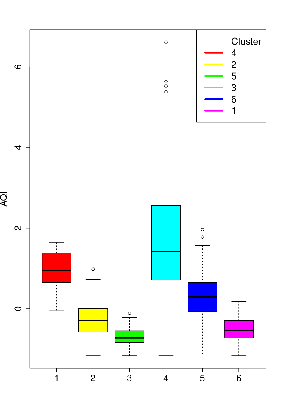
Figure S.7 displays three different predictive laws that correspond to different locations: Sacramento, which shows the lowest predicted values of AQI, New York, where the environmental conditions are worse, and Monterrey, that presents an intermediate situation.


Similarly as for the Biopics dataset, we compare the inference under our model with the linear dependent Dirichlet process mixture model introduced in De Iorio et al. (2004). Prior information is fixed as follows: is distributed according to the distribution for Test , so that the prior mean and variance of are 7.15 and 36, respectively, i.e. the prior of is vague. On the other hand, in Test the mass parameter of the Dirichlet process is set equal to 0.15 such that and , which approximately matches the prior information given on (mean 1.996 and variance 1.29). The baseline distribution is a multivariate Gaussian with mean vector 0 and a random covariance matrix which is given a non-informative prior and the hyperparameters of the inverse-gamma distribution for the variances of the mixture components are such that prior mean and variance are equal to 5 and 1, respectively. Posterior summaries can be found in Table S.10.
| Test | Var | MSE | LPML | |
|---|---|---|---|---|
| 5.14 | 0.38 | 827.72 | -1100.73 | |
| 5.03 | 0.16 | 827.04 | -1100.06 |
S.6 Additional plots
- •
- •
Figure S.9 displays the value of corresponding to the Gaussian spectral density where and varies as in the legend. The vertical dashed line represents the upper limit of the set . The approximation for is perfectly adhered to when is small. The higher the is, the slower is the decay rate of the function .
- •
Figure S.10 refers to Section 4.2 of the paper, where we considered a simulated dataset with three covariates. Predictive distributions corresponding to the 12 different reference values of the covariates are shown. The simulation truth can be found in Figure 1 of Müller et al. (2011).
- •
- •


References
- Affandi et al. (2013) Affandi, R. H., Fox, E., and Taskar, B. (2013). “Approximate inference in continuous determinantal processes.” In Advances in Neural Information Processing Systems, 1430–1438.
- Affandi et al. (2014) Affandi, R. H., Fox, E. B., Adams, R. P., and Taskar, B. (2014). “Learning the Parameters of Determinantal Point Process Kernels.” In ICML, 1224–1232.
- Bardenet and Titsias (2015) Bardenet, R. and Titsias, M. (2015). “Inference for determinantal point processes without spectral knowledge.” In Advances in Neural Information Processing Systems, 3393–3401.
- Binder (1978) Binder, D. A. (1978). “Bayesian cluster analysis.” Biometrika, 65, 31–38.
- Biscio and Lavancier (2016) Biscio, C. A. N. and Lavancier, F. (2016). “Quantifying repulsiveness of determinantal point processes.” Bernoulli, 22, 2001–2028.
- Biscio and Lavancier (2017) — (2017). “Contrast estimation for parametric stationary determinantal point processes.” Scandinavian Journal of Statistics, 44, 204–229.
- Daley and Vere-Jones (2003) Daley, D. J. and Vere-Jones, D. (2003). “Basic Properties of the Poisson Process.” An Introduction to the Theory of Point Processes: Volume I: Elementary Theory and Methods, 19–40.
- Daley and Vere-Jones (2007) — (2007). An introduction to the theory of point processes: volume II: general theory and structure. Springer.
- De Iorio et al. (2004) De Iorio, M., Müller, P., Rosner, G. L., and MacEachern, S. N. (2004). “An ANOVA model for dependent random measures.” Journal of the American Statistical Association, 99, 205–215.
- Ferguson (1983) Ferguson, T. S. (1983). “Bayesian density estimation by mixtures of normal distributions.” In M. H. Rizvi, J. R. and Siegmund, D. (eds.), Recent Advances in Statistics: Papers in Honor of Herman Chernoff on his Sixtieth Birthday, 287–302. Academic Press.
- Frühwirth-Schnatter (2006) Frühwirth-Schnatter, S. (2006). Finite mixture and Markov switching models. Springer Series in Statistics. Springer, New York.
- Fúquene et al. (2016)
Fúquene, J., Steel, M., and Rossell, D. (2016).
“On choosing mixture components via non-local priors.”
URL http://arxiv.org/abs/1604.00314v1 - Ishwaran and James (2001) Ishwaran, H. and James, L. F. (2001). “Gibbs sampling methods for stick-breaking priors.” Journal of the American Statistical Association, 96, 161–173.
- Ismay and Chunn (2017)
Ismay, C. and Chunn, J. (2017).
fivethirtyeight: Data and Code Behind the Stories and
Interactives at ’FiveThirtyEight’.
R package version 0.1.0.
URL https://CRAN.R-project.org/package=fivethirtyeight - Jara and Hanson (2011) Jara, A. and Hanson, T. E. (2011). “A class of mixtures of dependent tail-free processes.” Biometrika, 98, 553–566.
- Jara et al. (2011) Jara, A., Hanson, T. E., Quintana, F. A., Müller, P., and Rosner, G. L. (2011). “DPpackage: Bayesian semi-and nonparametric modeling in R.” Journal of Statistical Software, 40, 1–30.
- Kulesza and Taskar (2012) Kulesza, A. and Taskar, B. (2012). “Determinantal point processes for machine learning.” Foundations and Trends® in Machine Learning, 5, 123–286.
- Lau and Green (2007) Lau, J. W. and Green, P. J. (2007). “Bayesian model-based clustering procedures.” Journal of Computational and Graphical Statistics, 16, 526–558.
- Lavancier et al. (2015) Lavancier, F., Møller, J., and Rubak, E. (2015). “Determinantal point process models and statistical inference: Extended version.” Journal of the Royal Statistical Society: Series B (Statistical Methodology), 77, 853–877.
- Lo (1984) Lo, A. Y. (1984). “On a class of Bayesian nonparametric estimates: I. Density estimates.” The Annals of Statistics, 12, 351–357.
- Macchi (1975) Macchi, O. (1975). “The coincidence approach to stochastic point processes.” Advances in Applied Probability, 83–122.
- Malsiner-Walli et al. (2016) Malsiner-Walli, G., Frühwirth-Schnatter, S., and Grün, B. (2016). “Model-based clustering based on sparse finite Gaussian mixtures.” Statistics and Computing, 26, 303–324.
- McLachlan and Peel (2005) McLachlan, G. and Peel, D. (2005). Finite Mixture Models. John Wiley & Sons, Inc.
- Miller and Harrison (2013) Miller, J. W. and Harrison, M. T. (2013). “A simple example of Dirichlet process mixture inconsistency for the number of components.” In Advances in neural information processing systems, 199–206.
- Miller and Harrison (2017) — (2017). “Mixture models with a prior on the number of components.” Journal of the American Statistical Association, (In Press).
- Møller and Waagepetersen (2007) Møller, J. and Waagepetersen, R. P. (2007). “Modern statistics for spatial point processes.” Scandinavian Journal of Statistics, 34, 643–684.
- Müller et al. (2011) Müller, P., Quintana, F., and Rosner, G. L. (2011). “A product partition model with regression on covariates.” Journal of Computational and Graphical Statistics, 20, 260–278.
- Norets (2015) Norets, A. (2015). “Optimal Retrospective Sampling for a Class of Variable Dimen-sion Models.” Unpublished manuscript, Brown University, available at http://www. brown. edu/Departments/Economics/Faculty/Andriy_Norets/papers/optretrsampling. pdf.
- Petralia et al. (2012)
Petralia, F., Rao, V., and Dunson, D. B. (2012).
“Repulsive Mixtures.”
In Pereira, F., Burges, C., Bottou, L., and Weinberger, K. (eds.),
Advances in Neural Information Processing Systems 25, 1889–1897.
Curran Associates, Inc.
URL http://papers.nips.cc/paper/4589-repulsive-mixtures.pdf - Quinlan et al. (2017)
Quinlan, J. J., Quintana, F. A., and Page, G. L. (2017).
“Parsimonious Hierarchical Modeling Using Repulsive
Distributions.”
URL https://arxiv.org/abs/1701.04457v1 - Richardson and Green (1997) Richardson, S. and Green, P. J. (1997). “On Bayesian analysis of mixtures with an unknown number of components (with discussion).” Journal of the Royal Statistical Society: series B (statistical methodology), 59, 731–792.
- Roberts and Rosenthal (2009) Roberts, G. O. and Rosenthal, J. S. (2009). “Examples of adaptive MCMC.” Journal of Computational and Graphical Statistics, 18, 349–367.
- Rousseau and Mengersen (2011) Rousseau, J. and Mengersen, K. (2011). “Asymptotic behaviour of the posterior distribution in overfitted mixture models.” Journal of the Royal Statistical Society: Series B (Statistical Methodology), 73, 689–710.
- Shirota and Gelfand (2016) Shirota, S. and Gelfand, A. (2016). “Approximate Bayesian Computation and Model Validation for Repulsive Spatial Point Processes.” arXiv preprint arXiv:1604.07027.
- Xu et al. (2016) Xu, Y., Müller, P., and Telesca, D. (2016). “Bayesian Inference for Latent Biological Structure with Determinantal Point Processes (DPP).” Biometrics, 72, 955–964.
- Zellner (1986) Zellner, A. (1986). “On assessing prior distributions and Bayesian regression analysis with g-prior distributions.” Bayesian inference and decision techniques: Essays in Honor of Bruno De Finetti, 6, 233–243.