Reverse engineering protocols for controlling spin dynamics

We consider a spin 1/2 in an initial state $|\psi(0)\rangle$. Its time evolution is encapsulated in the evolution operator $U(t)$: $|\psi(t)\rangle=U(t)|\psi(0)\rangle$. The most general form for $U$ is a 2$\times$2 complex matrix whose coefficients are partially related to ensure its unitary property. Denoting $u_{ij}=\rho_{ij}e^{i\varphi_{ij}}$, the coefficients of $U$ shall fulfill the following relations $\varphi_{12}=\varphi_{21}\equiv\varphi$, $\rho_{12}=\rho_{21}\equiv\rho$, $\rho_{11}=\rho_{22}\equiv r$ and $\varphi_{11}+\varphi_{22}=2\varphi+\pi$. The most general form of $U$ therefore reads

where the variables $r$, $\varphi_{11}$ and $\varphi$ are time-dependent. The reverse engineering protocol consists in shaping in time the three variables $r$, $\varphi_{11}$ and $\varphi$ to ensure the transformation $|\psi(0)\rangle\longrightarrow|\psi(t_{f})\rangle=|\psi_{\rm target}\rangle$. The Schrödinger equation $i\hbar\partial_{t}|\psi(t)\rangle=H|\psi(t)\rangle$ implies that $H=i\hbar\dot{U}U^{\dagger}$. The expansion of $H$ on the Pauli matrices $\sigma_{i}$ ($i=x,y,z$) gives the time-dependent magnetic field components that should be implemented in order to follow the desired trajectory: $H=-\gamma_{1}{\bf s}_{1}\cdot{\bf B}(t)=-\gamma_{1}\hbar{\bm{\sigma}}\cdot{\bf B}(t)/2$ with

where $\gamma_{1}$ is the gyromagnetic factor and $\Phi=\varphi-\varphi_{11}$ the relative phase. We conclude that only two parameters are relevant in this case $r(t)$ and $\Phi(t)$. This form generally contains the particular results deduced from other methods such as the tracking transitionless algorithm and the dynamical invariant approach [19], see also Refs. [27, 28].

As a simple example, let’s work out the simplest form of the magnetic field components to ensure the spin flip of the spin. The wave function reads $|\psi(t)\rangle=r(t)e^{i\varphi_{11}(t)}|+\rangle+\sqrt{1-r^{2}(t)}e^{i\varphi(t)}|-\rangle$, where $|\pm\rangle$ are the eigenstates of $\sigma_{z}$ with eigenvalues $\pm 1$, corresponding to the spin up and down. To ensure the spin flip from $|+\rangle$ to $|-\rangle$ in an amount of time $t_{f}$, we need to fulfill the following boundary conditions, $r(0)=1$ and $r(t_{f})=0$. To avoid the divergence of denominators, we choose $\Phi=0$ and $r(t)=\cos(\theta(t))$ with $\theta(0)=0$ and $\theta(t_{f})=\pi/2$. We find $B_{x}=0$ and $B_{z}=0$, and a solution that contains the famous $\pi$-pulse solution with a constant magnetic field $B^{0}_{y}=\pi/(\gamma_{1}t_{f})$. The general method that we have worked out enables one to have any type of final state, including superposition of states.

Another strategy consists in using an exact semiclassical approach based on the phase-modulus equations, commonly referred to as the Modeling representation. To derive the corresponding set of coupled equations we start by introducing the general form $|\psi(t)\rangle=a(t)|+\rangle+b(t)|-\rangle$ into the Schrödinger equation in the presence of a time-dependent magnetic field:

Let’s rewrite the coefficients $a$ and $b$ in modulus-phase representation $a(t)=\sqrt{n_{a}(t)}e^{i\varphi_{a}(t)}$, $b(t)=\sqrt{n_{a}(t)}e^{i\varphi_{b}(t)}$. The two previous complex equations can be recast as a Hamiltonian problem for the conjugate variables $(n_{a},\varphi_{a})$ and $(n_{b},\varphi_{b})$: $\dot{n}_{i}=-\partial_{\varphi_{i}}H$, $\dot{\varphi}_{i}=\partial_{n_{i}}H$ with ($i=a,b$). It is convenient to introduce the relative variables $\Delta_{n}(t)=n_{a}(t)-n_{b}(t)$ and $\theta(t)=\varphi_{a}(t)-\varphi_{b}(t)$. The expression of the Hamiltonian now reads

and the dynamics is given by the two scalar equations

From the evolution of $\Delta_{n}$ and $\theta$, we can infer the components of the magnetic field. For instance,

Alternatively, we can work out the equations of motion for the mean value of the spin

In the following, we note ${\bf S}_{1}=2\langle{\bf s}_{1}\rangle/\hbar$ and use the spherical coordinates to describe the motion of the spin on the Bloch sphere: ${\bf S}_{1}(\sin\theta(t)\cos\varphi(t),\sin\theta(t)\sin\varphi(t),\cos\theta(t))$. To work out our reverse protocol, we calculate the left-hand side of precession equations (7)

Combining Eqs. (8)-(10), we get

from which we infer the expression of the transverse magnetic field components. With this set of equations we already obtain a class of solution by setting $B_{x}=B_{z}=0$ and $\varphi=0$, we find $\dot{\theta}=\gamma_{1}B_{y}$. The reverse engineering protocol consists here in choosing for $\theta(t)$ a function that obeys the boundary conditions $\theta(0)=0$ and $\theta(t_{f})=\pi$, and to infer from it the expression for $B_{y}(t)$. We can readily recover here also the $\pi$-pulse solution.

It is interesting to let the possibility to shape any curve on the Bloch sphere [30]. For this purpose, we need non trivial dependence of both $\theta(t)$ and $\varphi(t)$. However, as suggested by Eqs. (11) and (12), we can engineer only transverse magnetic field components and impose the variation of the longitudinal magnetic field component. This choice amounts to using explicitly the non uniqueness of the solution. The solution is then quite simple, we set the evolution of $\theta(t)$, $\varphi(t)$ and $B_{z}(t)$ according to our boundary conditions. We have to be careful since we need to avoid divergences. This means that we have to take care of the terms having a $\tan\theta$. This latter terms diverge for $\theta=\pi/2$, at time $t=t^{*}$ for which $\theta(t^{*})=\pi/2$. To compensate for this divergence, we have to cancel also $\dot{\varphi}(t^{*})=0$ and $B_{1z}(t^{*})=0$. A way out for the last term consists in choosing $B_{1z}(t)=B_{0}\cos(\theta(t))$. The set of equations (11) and (12) then reads

Consider the following example, we want to spin flip the spin from $|+\rangle$ to $|-\rangle$ in an amount of time $t=t_{f}$. For convenience, we use in the following the dimensionless time $s=t/t_{f}$. We use the boundary conditions $\theta(0)=0$ and $\theta(1)=\pi$. The simplest polynomial interpolation between those two boundary conditions is $\theta(s)=\pi s$. In this case, $s^{*}=1/2$. The boundary conditions for $\varphi$ are therefore $\varphi(0)=0$, $\varphi(1)=0$ and $\dot{\varphi}(1/2)=0$. We choose here a polynomial ansatz $\varphi(s)=s-s^{2}$ to fulfill those conditions. Equations (13) and (14) take then the simple form

Figures (1a) and (1b) provide respectively the evolution of the components of the magnetic field and of the spin. The choice of smooth polynomial ansatz for the reverse engineering protocol generates a smooth solution. As intuitively expected, the shorter $t_{f}$, the larger the variation. This feature can be seen directly on Eqs. (15) and (16) through the $1/t_{f}$ factors.

In conclusion of this section, we have shown that different formulations of the same problem yield different class of solutions. Within a given formulation, there is an infinitely large number of solutions for given boundary conditions. Those observations are useful to setup protocols for which we will add more constraints. In the following, we discuss the simultaneous spin flip of two spin having different gyromagnetic factors and the design of magnetic field trajectories that ensure an optimal spin flip fidelity robust against the value of the exact value of the gyromagnetic factor. We will focus on the precession equations which presents the advantage of a direct possible visualization of the spin trajectory on the Bloch sphere.

We now consider a second spin ${\bf S}_{2}$ having a different gyromagnetic factor $\gamma_{2}$ (we assume that there is no interactions between the two spins). To setup the reverse engineering protocol allowing to control both spins with the same time-dependent magnetic field, we proceed in the following manner: we enlarge the space of functions that flip the first spin, and search for the subset of parameters that also ensure the spin flip of the second spin. We shall use the same variation as previously for $\theta$ ($=\pi s$) but a more involved $\varphi(s)$ ansatz with two free parameters, $\kappa$ and $\eta$: $\varphi(s)=\kappa\left[s+(\eta-1)s^{2}-2\eta s^{3}+\eta s^{4}\right]$. This interpolating function fulfills the required boundary conditions $\varphi(0)=0$, $\varphi(1)=0$ and $\dot{\varphi}(1/2)=0$. Using Eqs. (13) and (14), we can readily infer the time-dependent components of the magnetic field that one should apply.

In Fig. 2, we plot $\Delta=1-|\langle-|\psi(t_{f})\rangle|^{2}=(1+S_{2z})/2$ as a function of the two parameters $\gamma_{2}/\gamma_{1}$ and $\eta$, and this for different values of $\kappa$. $\Delta$ provides a direct measurement of the projection of the spin on the $z$ axis at the end of the transformation. The blue zone are those for which we approach the target of a perfect reversing of spin two. This calculation shows (i) that whatever is the ratio $\gamma_{2}/\gamma_{1}$ there exists a couple of $(\eta,\kappa)$ parameters that will ensure a perfect rotation of the two spins despite the fact that their coupling strength to the magnetic field is different and (ii) the existence of dense blue zones (for $\gamma_{2}\sim\gamma_{1}$) for which the rotation for both spin can be very good, this feature is the one required for robustness against dispersion of the values of $\gamma_{2}$ (see below). Actually, the existence of many curves with minimum values of $\Delta$ in Fig. 2 means that we can simultaneously spin flip many spins having different gyromagnetic factors with the appropriate magnetic field. An example is depicted in Fig. 3 for three different spins where we have represented on the Bloch sphere the time-evolution of each spin. Interestingly, our protocol generates loops on the Bloch sphere to ensure that all spin trajectories end up at the opposite pole at the same time. The one loop trajectory is reminiscent of the spin echo technique but is here generated automatically by our protocol.

The reverse engineering protocol is well adapted to add further constraints. An important issue is to design spin flips protocols that are robust against the dispersion in the parameters governing the time evolution of the system. A standard example is provided by the dispersion of Larmor frequencies of an ensemble of two-level systems in liquid and solid NMR experiments [6]. This question is important for the implementation of quantum computing algorithm [40, 41].

To address this issue, we introduce $\Lambda(\epsilon)$ which measures an average distance towards the exact spin flip by averaging the different probabilities of remaining in the initial state in an interval of size $2\bar{\gamma}\epsilon$ about the mean gyromagnetic factor $\bar{\gamma}$ under consideration:

Figure 4 shows the decimal logarithm of the robustness function $\Lambda$ as a function of $\kappa$ where $\epsilon=0.01$ and $\eta=20$ is fixed. We observe the existence of a set of discrete “magic” values for $\kappa$ that ensures an optimal spin flips. The quality of the spin flips increases with the value of the magic $\kappa$ value. For instance, we get $\log_{10}[\Lambda(\epsilon=0.01)]=-7.8816$ for the first magic value $\kappa=2.0564$, $\log_{10}[\Lambda(\epsilon=0.01)]=-8.7127$ for $\kappa=3.262$. We have also represented the evolution of the second spin on the Bloch sphere in the inset of Fig. 4 for $\kappa=9.1892$, which corresponds to $\log_{10}[\Lambda(\epsilon=0.01)]=-9.4297$.

For a given time duration $t_{f}$ of the process, the robustness increases at the expense of an increasingly large transient magnetic field amplitude. The use of high optimal values of magic $\kappa$ generates many rotations of the spin on the Bloch sphere (see the inset of Fig. 4). This is not surprising since it simply generalizes somehow the spin echo technique.

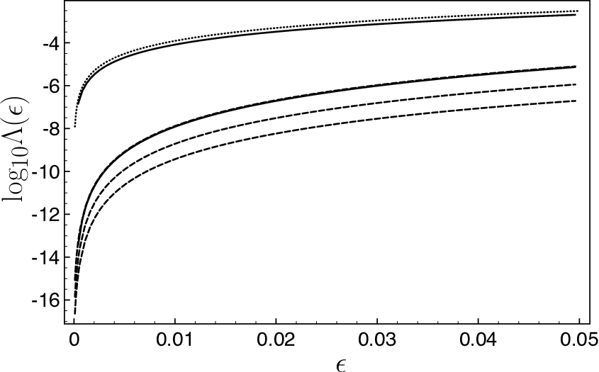
Figure 5 summarizes the robustness functions of different spin flip protocols for gyromagnetic factors spanning the interval $2\bar{\gamma}\epsilon$ about the mean value $\bar{\gamma}$. It compares the performance of (i) the simple $\pi-$pulse designed for the mean value $\bar{\gamma}$ and whose explicit expression is derived in Appendix, (ii) the spin echo technique (see Appendix) and different reverse engineering protocols. We include those latter protocols for a non magic value of the $\kappa$ parameter and for three magic values. The first magic value is already competitive with the spin echo technique (nearly superposition of the two corresponding robustness function). The larger magic values clearly improve efficiently the fidelity of the spin flip operation on the whole interval investigated here (up to 5% difference of the gyromagnetic factor).

The method presented in the previous sections can be readily generalized for other requirements. One could spin flip spin 1 and require for the spin 2 to end up in the horizontal plane of the Bloch sphere (superposition of state up and down with the same weight).

To confirm such possibilities offered by our extended space of parameter, we fix the ratio $\gamma_{2}/\gamma_{1}$, and plot the new $\Delta$ ($=S_{2z}$) function as a function of both parameters $\eta$ and $\kappa$. An example is provided in Fig. 6a for $\gamma_{2}/\gamma_{1}=0.5$. The two cut of the 2D plot (Fig. 6b) taken for two values of the $\eta$ parameter shows explicitly the existence of two values of $\kappa$ that ensures an optimal spin flip of spin 1 and that rotate spin 2 in the equatorial plane of the Bloch sphere. For instance, the optimal parameters are here: for $\eta=2$, $\kappa=4.6936$ with $\log_{10}(S_{2z})=-12.5451$ and for $\eta=3$, $\kappa=3.799$ with $\log_{10}(S_{2z})=-12.8491$.

Our method is generic. For instance with $\gamma_{1}=3$ and $\gamma_{2}=1$, our protocol also provides an optimal solution for the same target states. As an example, we find for $\eta=8$, $\kappa=5.429$ with $\log_{10}(S_{2z})=-12.6294$.

Consider a magnetic field function ${\bf B}_{0}(t)$ that solves simultaneously the equations (7) for spin 1 of gyromagnetic factor $\gamma_{1}$ and spin 2 of gyromagnetic factor $\gamma_{2}$ for the desired target states. It obeys

In the presence of isotropic interactions ($V^{(is)}_{\rm int}=\mu\bf s_{1}\cdot\bf s_{2}$), we search the magnetic field function ${\bf B}(t)$ that one should apply to reach the same target states. We therefore have to solve

Let’s search for a solution of the form ${\bf B}(t)={\bf B}_{0}(t)+\alpha{\bf S}_{1}+\beta{\bf S}_{2}$, where $\alpha$ and $\beta$ are two constant parameters that need to be determined. We have

Choosing $\beta=\mu/\gamma_{1}$ and $\alpha=\mu/\gamma_{2}$, we now have to solve the set of equations

and we know the solution ${\bf S}_{1}={\bf S}_{1}^{0}$ and ${\bf S}_{2}={\bf S}_{2}^{0}$. We conclude that the system (19) admits the solution ${\bf S}_{1}={\bf S}_{1}^{0}$ and ${\bf S}_{2}={\bf S}_{2}^{0}$ with a magnetic field that varies as

In other words, once we have a solution for two independent spins (including in the case of two different gyromagnetic factors) we have also the solution for two spins that interact through an isotropic interaction potential of the form $V^{(is)}_{\rm int}=\mu\bf s_{1}\cdot\bf s_{2}$ whatever is the strength of interaction between the two spins. However, one can never rich the Bell state $|{\rm Bell}\rangle=(|+-\rangle+|-+\rangle)/\sqrt{2}$ with isotropic interactions.

To reach such a state, one needs anisotropic interactions. The Hamiltonian of two identical spins 1/2 therefore reads

It is block diagonal in the basis that classifies the states by their angular momentum $|++\rangle$, $|{\rm Bell}\rangle$ and $|A\rangle=(|+-\rangle-|-+\rangle)/\sqrt{2}$.

As we are interested in the simultaneous spin flip of the two interacting spins or in the generation of the Bell state, we search for a solution in the subspace of angular momentum $J=1$: $|\psi(t)\rangle=a(t)|++\rangle+b(t)|{\rm Bell}\rangle+c(t)|--\rangle$. The time dependent complex coefficients $a(t)$, $b(t)$ and $c(t)$ obey the set of linearly coupled equations

where $\gamma$ is the gyromagnetic factor and $B_{\pm}=B_{x}\pm iB_{y}$.

The adiabatic passage techniques shows that the dynamics is amenable to a 2$\times 2$ submatrix involving only $a$ and $b$ variables [45]. The adiabaticity requires a transformation on a typical time scale of $30\hbar/\xi$. The shortcuts to adiabaticity techniques can be used in this subspace to accelerate the transition from the fully polarized state $|++\rangle$ to the Bell state $|{\rm Bell}\rangle$ [46].

For this purpose, we search for a solution that corresponds to a transverse rotating magnetic field whose amplitude varies as a function of time: $\gamma B_{x}(t)=B(t)\cos(\omega t)$ and $\gamma B_{y}(t)=B(t)\sin(\omega t)$. The sub matrix on $a$ and $b$ variables can be recast in a symmetric form within the interaction picture

where the diagonal time dependent coefficient is related to the longitudinal magnetic field component: $\Delta(t)=\gamma B_{z}(t)-\omega+2\xi$. A convenient and classical method to implement reverse engineering in this context relies on the use of dynamical invariants. This method simply consists in determining a matrix $I(t)$ that fulfills the following relation

with the boundary conditions $[H_{I}(0),I(0)]=[H_{I}(t_{f}),I(t_{f})]=0$. To find this matrix $I(t)$, we use the Lie algebra operators and expand $I(t)$ on the Pauli matrices: $I(t)={\bf u}\cdot\bm{\sigma}$ where ${\bf u}$ is a unit vector of spherical angles $(\theta,\varphi)$. The eigenstate of $I(t)$, $|\phi_{+}(t)\rangle=\cos(\theta/2)e^{i\varphi}|++\rangle+\sin(\theta/2)|{\rm Bell}\rangle$, is also the eigenstate of $H_{I}(t)$ for initial and final time according to the commutation relations for boundary conditions. The reverse engineer method amounts to fixing the evolution of the vector ${\bf u}$ in order to interpolated the evolution between the initial state $|\phi_{+}(0)\rangle\propto|++\rangle$ and the desired final state $|\phi_{+}(t_{f})\rangle\propto|{\rm Bell}\rangle$. To this end, the commutation relations shall be transposed as boundary conditions for the time dependent variables $\theta(t)$ and $\varphi(t)$: $\theta(0)=0$, $\theta(t_{f})=-\pi$ , $\dot{\theta}(0)=0$, $\dot{\theta}(t_{f})=0$, $\varphi(0)=-\pi/2$, $\varphi(t_{f})=-\pi/2$, $\varphi(t_{f}/2)=-\pi/2$, $\dot{\varphi}(0)=-\pi/t_{f}$, and $\dot{\varphi}(t_{f})=\pi/t_{f}$. From Eq. (28), we obtain the relation between the Hamiltonian variables and the angles of ${\bf u}$, namely,

We infer the value of $B(t)$ and $B_{z}(t)$, using the polynomial interpolation of minimum order according to the boundary conditions for the $\theta(t)$ and $\varphi(t)$ variables.

In Fig. 7, we plot the fidelity towards the desired Bell state at final time by solving the set of Eqs. (24)-(26) with the magnetic field derived from the preceding approach. We find an improvement of at least one order of magnitude on the time required to reach the Bell state with high fidelity compared to the adiabatic evolution. As intuitively expected, it is impossible to accelerate to arbitrary short time. This is due to the finite value of the coupling (the $\xi$ parameter) that we kept fixed and which imposes a timescale $\hbar/\xi$.

Interestingly, this method can be readily generalized to more spins in a symmetric configuration. For instance, with three spins at the vertex of an equilateral triangle the same approach enables one to design in time the required fast evolution of the magnetic field components to drive the system from the fully polarized state $|+++\rangle$ to the ${\rm W}$ entangled state $=(|-++\rangle+|+-+\rangle+|++-\rangle)/\sqrt{3}$ (see dashed line in Fig. 7).

References

- [1] D. Awschalom, D. Loss, and N. Samarth, Semiconductor Spintronics and Quantum Computation (Springer, Berlin, 2002).
- [2] B. W. Shore, Manipulating quantum structures using laser pulses (Cambridge, New York, 2011).
- [3] K. Bergmann, H. Theuer, and B. W. Shore, Rev. Mod. Phys. 70, 1003 (1998).
- [4] P. Král, I. Thanopulos, and M. Shapiro, Rev. Mod. Phys. 79, 53 (2007).
- [5] N. V. Vitanov, A. A. Rangelov, B. W. Shore, and K. Bergmann, Rev. Mod. Phys. 89, 015006 (2017)
- [6] M. H. Levitt, Prog. Nucl. Magn. Renos. Spectrosc. 18, 61 (1986).
- [7] B. T. Torosov, S. Guérin, and N. V. Vitanov, Phys. Rev. Lett. 106, 233001 (2011).
- [8] I. R. Solá, V. S. Malinovsky, and D. J. Tannor, Phys. Rev. A 60, 3081 (1999).
- [9] U. Boscain, G. Charlot, J.-P. Gauthier, S. Guérin, and H.-R. Jauslin, J. Math. Phys. 43, 2107 (2002).
- [10] F. Albertini and D. D’Alessandro, J. Math. Phys. 56, 1893 (2015).
- [11] G. G. S. Vasilev, A. Kuhn, and N. V. Vitanov, Phys. Rev. A 80, 013417 (2009).
- [12] E. Torrontegui, S. Ibáñez, X. Chen, A. Ruschhaupt, D. Guéry-Odelin and J. G. Muga, Phys. Rev. A 83, 013415 (2011).
- [13] D. Guéry-Odelin and J. G. Muga, Phys. Rev. A 90, 063425 (2014).
- [14] Q. Zhang, X. Chen and D. Guéry-Odelin, Phys. Rev. A, 92, 043410 (2015).
- [15] S. Martinez-Garaot, P. Palmero, J. G. Muga and D. Guéry-Odelin, Phys. Rev. A 94, 063418( 2016).
- [16] D. Guéry-Odelin, J. G. Muga, M. J. Ruiz-Montero and E. Trizac, Phys. Rev. Lett. 112, 180602 (2014).
- [17] I. A. Martinez, A. Petrosyan, D. Guéry-Odelin, E. Trizac, and S. Ciliberto, Nat. Phys., 12, 843 (2016).
- [18] A. L. Cunuder, I. A. Mart¨ªnez, A. Petrosyan, D. Guéry-Odelin, E. Trizac, and S. Ciliberto, Appl. Phys. Lett. 109, 113502 (2016).
- [19] E. Torrontegui, S. Ibáñez, S. Martínez-Garaot, M. Modugno, A. del Campo, D. Guéy-Odelin, A. Ruschhaupt, X. Chen, and J. G. Muga, Adv. At. Mol. Opt. Phys. 62, 117 (2013).
- [20] S. Deffner, C. Jarzynski, and A. del Campo, Phys. Rev. X 4, 021013 (2014).
- [21] A. Emmanouilidou, X.-G. Zhao, P. Ao, and Q. Niu, Phys. Rev. Lett. 85, 1626 (2000).
- [22] Y. Ban, X. Chen, E. Y. Sherman, and J. G. Muga, Phys. Rev. Lett. 109, 206602 (2012).
- [23] Z.-G. Song, H. Wu, S. Wang, Y. Ban, and X. Chen, arXiv:1703.03601.
- [24] A. Ruschhaupt, X. Chen, D. Alonso, and J. G. Muga, New J. Phys. 14, 093040 (2012).
- [25] D. Daems, A. Ruschhaupt, D. Sugny, and S. Guérin Phys. Rev. Lett. 111, 050404 (2013).
- [26] X. J. Lu, X. Chen, A. Ruschhaupt, D. Alonso, S. Guérin, and J. G. Muga, Phys. Rev. A 88, 033406 (2013).
- [27] E. Barnes and S. Das Sarma, Phys. Rev. Lett 109, 060401 (2012); E. Barnes, Phys. Rev. A 88, 013818 (2013).
- [28] N. V. Vitanov and B. W. Shore, J. Phys. B: At. Mol. Opt. Phys. 48, 174008 (2015).
- [29] C. Sun, A. Saxena, and N. A. Sinitsyn, arXiv:1703.10271v1.
- [30] M. V. Berry J. Phys. A: Math. Theor. 42, 365303 (2009).
- [31] K. Takahashi Phys. Rev. E 87, 062117 (2013).
- [32] J.-F. Zhang, J. H. Shim, I. Niemeyer, T. Taniguchi, T. Teraji, H. Abe, S. Onoda, T. Yamamoto, T. Ohshima, J. Isoya, and D. Suter, Phys. Rev. Lett. 110, 240501 (2013).
- [33] M. Farzanehpour and I. V. Tokatly, Phys. Rev. A 93, 052515 (2016).
- [34] B. Wu and Q. Niu, Phys. Rev. A 61, 023402 (2000); J. Liu, L.-B. Fu, B.-Y. Ou, S.-G. Chen, D.-I. Choi, B. Wu, and Q. Niu, ibid. 66, 023404 (2002).
- [35] M. G. Bason, M. Viteau, N. Malossi, P. Huillery, E. Arimondo, D. Ciampini, R. Fazio, V. Giovannetti, R. Mannella, and O. Morsch, Nat. Phys. 8, 147 (2012).
- [36] Y.-A. Chen, S. D. Huber, S. Trotzky, I. Bloch, and E. Altman, Nat. Phys. 7, 61 (2010).
- [37] A. del Campo, Phys. Rev. Lett. 111, 100502 (2013).
- [38] H. Saberi, T. Opatrný, K. Molmer, A. del Campo, Phys. Rev. A 90, 060301(R) (2014).
- [39] X. Chen, Y. Ban, and G. C. Hegerfeldt, Phys. Rev. A 94, 023624 (2016).
- [40] M. D. Lukin and P. R. Hemmer, Phys. Rev. Lett. 84, 2818 (2000).
- [41] N. Ohlsson, R. K. Mohan and S. Kröll, Opt. Commun. 201, 71 (2002).
- [42] R. G. Unanyan, N. V. Vitanov, and K. Bergmann, Phys. Rev. Lett. 87, 137902 (2001).
- [43] S. Mancini and S. Bose, Phys. Rev. A 70, 022307 (2004).
- [44] S. J. Yun, J.-W. Kim, C. H. Nam, J. Phys. B: At. Mol. Opt. Phys. 48, 075501 (2015).
- [45] R. G. Unanyan, N. V. Vitanov, and K. Bergmann, Phys. Rev. Lett. 87, 137902 (2001).
- [46] K. Paul and A. K. Sarma, Phys. Rev. A 94, 052303 (2016)