A novel conductivity mechanism of highly disordered carbon systems based on an investigation of graph zeta function
Abstract
In the previous report [Phys. Rev. B 62 13812 (2000)], by proposing the mechanism under which electric conductivity is caused by the activational hopping conduction with the Wigner surmise of the level statistics, the temperature-dependent of electronic conductivity of a highly disordered carbon system was evaluated including apparent metal-insulator transition. Since the system consists of small pieces of graphite, it was assumed that the reason why the level statistics appears is due to the behavior of the quantum chaos in each granular graphite. In this article, we revise the assumption and show another origin of the Wigner surmise, which is more natural for the carbon system based on a recent investigation of graph zeta function in graph theory.
I Introduction
In the previous reports [20, 21], the temperature-dependence of the electric conductivity (TDEC) of activated carbon fibers (ACFs) was investigated, which are known as highly disordered systems (HDSs) [8]. A mechanism of activational hopping conductivity for the disordered systems was proposed that thermal excitations with the Wigner surmise,
| (I.1) |
contribute to the conductivity. The mechanism provides the TDEC which is in good agreement with the experimental results of Kuriyama [14] and reproduces the (apparent) metal-insulator transition in [15].
Further in [20, 21], it was microscopically assumed that the Wigner surmise comes from the quantum chaos in the small particles because the ACFs consists of small pieces of graphite [8]; each piece of small graphite might be regarded as a quantum box and it is known that its energy eigenvalue is described well by the random matrix theory (RMT) and obeys the Wigner surmise (I.1) [22].
In this article, we revise the assumption and employ another origin of the Wigner surmise based on the recent results of the graph theory on Ihara’s zeta function [25]. The new origin is much more natural for the ACFs.
The electrical and structural properties of the ACFs were studied by Kuriyama and Dresselhaus [14, 15] and others [8, 9]. Since the ACF consists of small pieces of graphite, the X-ray diffraction and Raman spectra show that the heat-treated process (HTP) of the ACFs modifies the structure and the size of the pieces drastically changes [8, 9]. Kuriyama studied the TDEC of the ACFs and its dependence on the HTP experimentally [14], and found the fact that if the density of states (DOS) of the activational energy is given by a -shape and the conductivity is proportional to the thermal activation, the estimation reproduces his own experimental results of the TDEC.
It implies that the previous reports [20, 21] gave a microscopic picture of Kuriyama’s mechanism based on the quantum chaos as mentioned above.
It is well-known that the RMT coming from the quantum chaos also represents the behaviors of the Riemann zeta function in the number theory [25].
Recently Newland showed numerically that even Ihara’s zeta function in the graph theory also obeys the Wigner surmise [25]. Since the zeta function is determined by the spectrum of the adjacency matrix (SAM) in graph theory, it was also found numerically that the SAM of a graph is also governed by the Wigner surmise. These results were obtained from the motivation of pure mathematics. However from a physical point of view, it means that the energy gaps of the tight binding model of certain materials with chemical bonding obey the Wigner surmise (I.1). Thus we employ this picture in this article.
II Results of the Previous report
Here we will review the formula in [20, 21] on the TDEC in HDCs or the ACFs with the temperature of the HTP as a parameter.
As mentioned in §I, by employing the Wigner surmise (I.1) as the DOS, the total conductivity is expressed by
| (II.1) |
where is a fitting parameter depending on , and weakly depends on the temperature , . Then (II.1) reproduces well the experimental results [14] including the insulator-metal transition [15] as in FIG. 1.

As mentioned in §I, it was considered in [20, 21] that the origin of the Wigner surmise (I.1) was quantum chaos for the quantum boxes since the graphite pieces of the ACF might be regarded as small granular particles. For example, the quantum system of stadium is governed by the RMT. The Wigner surmise naturally appears in the RMT since each level is repulsive in [1, 22].
III Electric structure of graphite
The electronic property of graphite has been studied well. The tight-binding approximation (TBA) of -electron distribution of graphite as a 2D honeycomb lattice was studied in [27, 5]. Coulson and Taylor also considered effects of overlap integrals and 3D effect [6]. Zunger investigated a more realistic model [28].
In these studies, the infinite size of lattice or pure crystal of graphite was assumed. On the other hand, as in [8, p.71] and [9], the ACFs consists of small pieces of graphite and the HTP of the ACFs modifies the structure and the size of the pieces drastically.
The boundary of the graphite piece is not stable due to dangling bonds. Since the phonon is easily excited there, the coherency of the electron wave function is loosed there. Since the ACF is considered as a collection of small graphite pieces, the electronic band structure is given as that of independent pieces as in [8, p.153-161].
In the picture, since the shape of the piece is crucial, we go back to the TBA as a simple approximation [23].
IV The TBA and theory of graph
We consider the electronic structure of the small graphite pieces in the framework of the TBA. For a given graph , e.g. FIG. 4, let the set of nodes in denoted by and that of edges in by . For the real numbers and [eV] [8, p.160], the hamiltonian of is given by where is the diagonal matrix and is the adjacency matrix of the graph ; for every , , and if there is an edge in otherwise vanishes [7, 3]. , , and are -matrices for . The spectrum of is determined by the SAM [7].
In the graph theory, Ihara’s zeta function and the SAM have been studied as a graph theoretic version of the Riemann hypothesis [13, 25]. As in [22], since many observations show that mathematical properties of the Riemann zeta function associated with Riemann hypothesis are expressed well by the RMT, the graph zeta function and SAM should be also described by the RMT. It is shown that for a certain (random) graph, the Wigner semicircle law governs the SAM [24, 25].
Further Newland, in his thesis 2005, showed by numerical computations that in a certain graph, the spectra of the adjacency matrices and Ihara’s zeta functions obey the Wigner surmise (I.1) [25, p.41].
The SAM of the infinite 2D graphite lattice or the honeycomb lattice was obtained by Coulson and Rushbrooke [5] and, later, was precisely studied by Horiguchi in terms of the lattice Green function method [10, 3]. The DOS is explicitly written by
| (IV.1) |
where is the Jacobi elliptic integral of the first kind and , as in FIG. 2. It is also noted that Ihara’s zeta function of the infinite lattice is related to the elliptic integral [4].

The SAM of a small piece of graphite asymptotically approaches to the DOS (IV.1) when its size approaches to . It is contrast to the fact that for a certain class of the random graph, the asymptotic behavior of the DOS obeys the semicircle law [24].
However it is expected that the density of the level-spacing of the SAM is determined by a function similar to the Wigner surmise (I.1) because 1) the degenerate states are naturally avoided if there is no global symmetry and 2) the average of the level spacings must be determined by the insertions of points into the region .
V Conductivity of the ACFs
Let us employ the ansatz that the level statistics of the graphite piece obeys the Wigner surmise (I.1). Though the gap of the first excited state from the Fermi level (the gap between HOMO (highest occupied molecular orbital) and LUMO (lowest unoccupied molecular orbital)) is concerned only, it is natural to assume that the gap also obeys the Wigner surmise (I.1) from recent development of the graph theory mentioned above [25].
In the framework of the TBA, the occupied states depend on the number of the carbon atoms and due to the spin effect; there is the gap if the number is even whereas the state is not filled if the number is odd. Though depending on the parity of each graphite piece, there appears the following picture as a large resistance case.

(a) (b)
Let us consider the hopping phenomena between two adjacency graphite pieces. As in illustrated in FIG. 3, in order that an electron in a piece hops to its adjacency one, the electron must jump to excited states as the first step. Under the electric field, the possibility of hopping is influenced and we have finite conductivity.
Let us consider that the ACF is arranged between two electrodes. From one electrode to another, there are possible electric paths [19, 20, 21]. Let be the local conductivity of adjacency graphite pieces belonging to the path . The conductivity along the path could be approximated by
Then the total conductivity is simply obtained by the summation over all paths, It means (II.1) and the above picture shows its microscopic origin.

(A1):50 (A2):50 (A3):50

(B1):100 (B2):100 (B3):98

(C1):199 (C2):202 (C3):201
VI Numerical Study
We, first, numerically showed the justification of the ansatz in §V for graphs given as FIG. 4 using the software Graphtea; we computed their SAM by solving numerically. Let the distribution of the SAM denoted by and that of level spacings by . The results are illustrated in FIG. 5, which shows that approach to (IV.1) asymptotically and is similar to due to the level repulsion. In other words, our ansatz in §V is natural. In fact, FIG. 5 exhibits that ’s are approximated by the Wigner surmise (I.1).
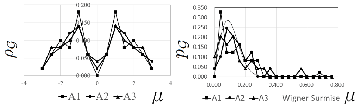
(a) (b)
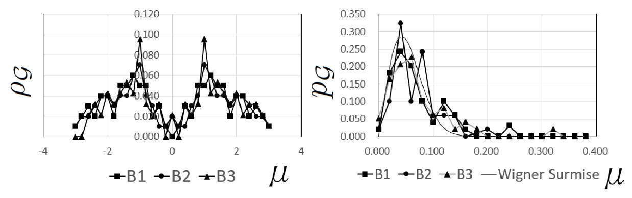
(c) (d)
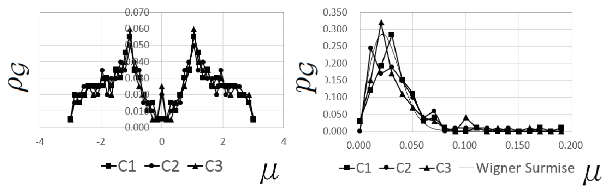
(e) (f)
We computed the center of the gravity for ’s, i.e., , and the effective for [eV] noting as in Table 1:
Table 1. Center of gravity of and [K]
1
2
3
average
[K]
A-type
0.136
0.135
0.134
0.135
5586
B-type
0.069
0.068
0.069
0.069
2842
C-type
0.035
0.035
0.034
0.035
1436
Using the least mean square method, the relation between and the number is evaluated as [K] from Table 1. With the estimation for the radius and [nm], the fitting parameters ’s in FIG. 1 are reduced to the effective radii ’s as in Table 2.
Table 2. and of the ACF
[K]
N
[nm]
case I
AS
180
3.2
case II
[∘C]
40
6.7
case III
[∘C]
20
9.5
case IV
[∘C]
0.1
1.3
Since X-ray analysis shows that there is 1.1[nm] peak which corresponds to the length along -axis of three stratified graphite sheets [8, 9]. Thus by considering 3D effect, ’s of case I-III in Table 2 should be divided by several numbers. From p.71 in [8], the structure of the ACF strongly depends on of HTP and especially around [∘C], the structure drastically changes and has 3D property as a kind of structural phase transition. However the critical temperature also depends on the material origin of the ACFs. Thus the ACF of case IV may have the 3D structure and if we use , . Then these estimations of ’s are compatible with TEM data in [8] and it also turns out that the (apparent) metal-insulator transition might come from the structural transition due to the HTP.
VII Discussions
In this article, we show that the SAM reproduces the conductivity of the disordered carbon system. We conclude that our picture is natural to the TDEC of the ACFs. In the series of works [11, 22, 18, 19], One of the authors (S.M.) has been showing that some of physical phenomena are expressed well by pure mathematical results. Since the SAM appears in theory of the graph zeta function which has been studied as a graph theoretic version of the Riemann hypothesis [13, 24, 25, 26], the TDC of the ACFs is one of such cases.
However the studies on the Wigner surmise of SAM are not sufficient. Especially the gap between HOMO and LUMO of pieces of graphite should be studied more systematically [17]. Further since there are studies of more realistic computation of electronic structure of graphite pieces [2, 3], it is expected that the statistical property of gaps for these systems is evaluated in future.
Since recently it is found that Ihara’s zeta functions naturally appears in quantum walks [12], it means that this investigation might show another possibility of quantum walk.
Acknowledgment: We are grateful to Professor Norio Konno for helpful discussions. We also acknowledge the graph software Graphtea developed in Graphlab in Sharif University of Technology. This work was supported by the Grant-in-Aid for Scientific Research (C) of Japan Society for the Promotion of Science (Grant No. 16K05187 (S.M.) and Grant No. 15K04985 (I.S.)).
References
- [1] M. V. Berry, Ann. Phys. (N.Y.) , 131 (1981) 163-216.
- [2] J. M. Carlsson, Computer-based modeling of novel carbon system and their properties, ed. by F. Catldo and P. Milani, p.79-128, Springer, New York, 2010.
- [3] A. H. Castro Neto, et. al, Rev. Mod. Phys., 81 (2009) 109-162.
- [4] B. Clair, Elec. J. Comb., 21 (2014) #P2.16.
- [5] C. A. Coulson and G. S. Rushbrooke, Proc. Roy. Soc. Edin., 62 (1948) 350-359.
- [6] C. A. Coulson and R. Taylor, Proc. Phys. Soc. A, 65 (1952) 815-825.
- [7] J. R. Dias, Molecular orbital calculations using chemical graph theory, Springer-Verlag, New York, 1993.
- [8] M. S. Dresselhaus, et al., Graphite fibers and filaments, Springer-Verlag, New York, 1988.
- [9] M. S. Dresselhaus, et al., Carbon, 30 (1992) 1065-73.
- [10] T. Horiguchi, J. Math. Phys., 19 (1972) 1411-1419.
- [11] Y. Ide, N. Konno, S. Matsutani, H. Mitsuhashi, to appear in Ann. Phys., arXiv:1610.02393.
- [12] N. Konno and I. Sato, Quantum Inf. Proc., 11 (2012) 341-349.
- [13] M. Kotani and T. Sunada, J. Math. Sci. Univ. Tokyo, 7 (2000) 7-25.
- [14] K. Kuriyama, Phys. Rev. B, 47 (1993) 12415-12419.
- [15] K. Kuriyama and M. S. Dresselhaus, J. Mater. Res. , 7 (1992) 940-945.
- [16] S. Matsutani, J. Geom. Symm. Phys, 17 (2010) 45-86.
- [17] S. Matsutani, in preparation.
- [18] S. Matsutani and Y. Onishi, Found. of Phys. Lett., 16 (2003) 325-341.
- [19] S. Matsutani and Y. Shimosako, Appl. Math. Modelling, 39 (2015) 7227-7243.
- [20] S. Matsutani and A. Suzuki, Phys. Lett. A, (1996) 216 178-82.
- [21] S. Matsutani and A. Suzuki, Phys. Rev. B, (2000) 62 13812-5.
- [22] M. L. Mehta, Random Matrices, revised and enlarged 2nd ed., Academic Press, Boston, 1991.
- [23] Y. V. Skrypnyk and V.M. Loktev, Low Temp. Phys., 42 (2016) 863-869.
- [24] T. Sunada, The discrete and the continuous, Sugaku Seminar, (in Japanese) (2001) 40 48-51.
- [25] A. Terras, Zeta functions of graphs, Cambridge, Cambridge, 2011.
- [26] A. B. Venkov and A. M. Nikitin, St. Petersburg Math. J., (1994) 5 419-484.
- [27] P. R. Wallace, Phys. Rev. B, 71 (1947) 622-632,
- [28] A. Zunger, Phys. Rev. B, 17 (1978) 626-641.