Modulation of Galactic Cosmic Rays in the Inner Heliosphere, comparing with PAMELA measurements
Abstract
We develop a numerical model to study the time-dependent modulation of galactic cosmic rays (GCRs) in the inner heliosphere. In the model a time-delayed modified Parker heliospheric magnetic field (HMF) and a new diffusion coefficient model, NLGCE-F, from Qin & Zhang (2014), are adopted. In addition, the latitudinal dependence of magnetic turbulence magnitude is assumed as from the observations of Ulysses, and the radial dependence is assumed as , where we choose an expression of as a function of the heliospheric current sheet (HCS) tilt angle. We show that the analytical expression used to describe the spatial variation of HMF turbulence magnitude agrees well with the Ulysses, Voyager 1, and Voyager 2 observations. By numerically calculating the modulation code we get the proton energy spectra as a function of time during the recent solar minimum, it is shown that the modulation results are consistent with the PAMELA measurements.
Keywords:
cosmic rays, modulation, turbulence, activity – Sun: heliosphereI Introduction
Galactic cosmic rays (GCRs) are modulated by solar wind irregularities while transporting inside the heliosphere. The physical mechanism of cosmic ray transport in the heliosphere is described by a well known Parker transport equation (TPE) [67],
| (1) |
where is the omni-directional cosmic ray distribution function, with the position, the particle momentum and the time. The distribution function is related to the differential intensity with respect to kinetic energy by . The terms on the right hand side include all the relevant transport processes, i.e., the outward convection by the solar wind velocity , the pitch-angle averaged drift velocity caused by irregularity in the global heliospheric magnetic field, is the symmetric part of the diffusion tensor which is diagnal in HMF-aligned coordinate system, and the adiabatic energy loss, which have been successfully illustrated by theoretical and numerical models [67, 105, 69, 91, 72, 107, see, e.g., ].
The past solar cycle (Cycle 24) was unusual with a prolonged periodicity, and the solar minimum conditions lasted until early 2010. During the solar minimum of 2006 to 2009, the averaged sunspot number (SSN) was reported to be the lowest since 1914 [82]. The solar polar field strength during the 2003-2004 solar maximum was especially weaker than previous three solar cycles [94]. The heliospheric magnetic field (HMF) reached 3 nT at 1 AU in 2009, the lowest value since 1963 [10]. The tilt angle () of the heliospheric current sheet (HCS) had a flatter decline than previous solar minimums [11]. It is also reported that the coronal mass ejection (CME) rates and the solar wind dynamic pressure in 2008-2009 were noticeably lower than that in 1997-1998 [99, 55]. These extreme solar minimum conditions resulted in a record high-level GCR intensity measured at Earth [59, 11]. Such a prolonged solar minimum provides a good chance to study the modulation of GCRs inside the heliosphere [58, 6, 76, 107, e.g.,].
The Payload for Antimatter-Matter Exploration and Light-nuclei Astrophysics (PAMELA) satellite experiment was designed to study the charged components of cosmic rays (CRs), among which antiparticles are focused. PAMELA has been taking data since it was launched in June 2006, and has brought plentiful scientific results about the heliosphere [8, 61, 34]. PAMELA measures precise cosmic ray proton and helium spectra in the rigidity range from GV to TV [4]. The energy spectra of protons and helium particles show different spectral indexes above 30 GV and both present a spectral hardening at about GV. The electron and positron energy spectra are measured up to GeV and GeV, respectively [3, 5]. PAMELA also measures the flux of Boron and Carbon as well as the boron-to-carbon (B/C) ratio which can be utilized to investigate the cosmic ray propagation processes [7]. Adriani et al. [6] presented precise galactic proton energy spectra in the range GeV for each Carrington rotation from July 2006 to January 2010. The observed proton spectra became progressively softer since July 2006. Later, Adriani et al. [9] reported precise electron spectra with a six-month interval at the same time period. Such precise CR energy spectra can be used to study physical processes of CR transport in the heliosphere, including convection, diffusion, drifts, and adiabatic energy changes.
The precise cosmic ray spectra measured by PAMELA instrument provides important information for people to understand the origin and propagation of GCRs. Voyager 1 was assumed to have crossed the heliopause (HP) at AU on August 2012 [101], cosmic ray spectra in the energy between MeV to MeV in the very local interstellar medium was then reported by Stone et al. [88]. The cosmic ray spectra data from PAMELA and Voyager 1 can be used to construct the very local interstellar spectrum [76, 63, 77, 97, 15, LIS, see e.g.,]. The LIS is important as the input spectrum in the solar modulation study. To understand the modulation processes during this unusual solar minimum, three-dimensional (3D) numerical models have been established to solve the Parker transport equation. Zhao et al. [107] used an empirical diffusion coefficient model according to Zhang [105] and incorporated a 3D wavy HCS. By reproducing the proton spectra observed by PAMELA and IMP 8 in previous two solar minima, they concluded that increased parallel diffusion and decreased perpendicular diffusion in polar direction caused by low magnetic turbulence might be the possible mechanism for the high GCR intensity in the past solar minimum, which is in contrast to the assumption of enhanced diffusion in the polar regions that was used to explain the observed Ulysses CR gradients [73, e.g.,]. Potgieter et al. [76] used a different diffusion coefficient model, in which modulation parameters vary as a function of time, in their numerical work. They successfully reproduced the PAMELA proton spectra for four selected periods and reported that this solar minimum was “diffusion dominated”, and that the modulation effects of particle drifts were less obvious but still played a significant role. Similar numerical model was also used to study the modulation of galactic electrons [77] and the modification effects of Parker HMF over the polar region Raath et al. [80].
Furthermore, due to the precise proton and electron spectra measured by PAMELA from 2006 to 2009 [6, 9], one is able to know the different modulation effects between protons and electrons, which is called the charge-sign-dependent modulation. In this past polarity solar minimum, low-energy protons were more sensitive to the changes of heliospheric conditions than low-energy electrons, such phenomenon can be reproduced only by incorporating drifts in the numerical model [27]. The PAMELA proton flux data were also used to study the spatial gradients in the inner heliosphere together with proton flux data from Ulysses COSPIN/KET. de Simone et al. [26] and Gieseler & Heber [36] used an empirical approach to calculate the radial and latitudinal gradients of protons during the past solar minimum. It is shown that the radial gradients are always positive while the latitudinal gradients are always negative as expected but with less magnitude than that predicted by earlier works [74]. Following de Simone et al. [26] and Gieseler & Heber [36], Vos & Potgieter [98] also used a numerical model to compute the spatial gradients of protons from 2006 to 2009. They concluded that although the drift effects were weaker than the predictions from those drift-dominated works due to the suppression by the excess diffusion, they still played an important role due to the significant decrease of HMF magnitude until the end of 2009.
Note that numerical models of modulation are usually solved in steady state, interplanetary conditions have to be determined with the solar activity some time before because of the limit of solar wind speed. Ndiitwani et al. [62] used a time-dependent two-dimensional (2D) numerical model to study CR modulation using PAMELA proton data in this unusual period. Smoothed monthly HMF and HCS, which were embedded in the solar wind plasma, were used to establish a realistic heliospheric conditions. Based on the work of Manuel et al. [52] and Potgieter et al. [76], Ndiitwani et al. [62] established a time-dependent diffusion coefficient model, in which the yearly time-dependent modulation parameters were obtained from the compound model [52] and the empirical model [76], respectively. However, Ndiitwani et al. [62] did not consider the variations of solar wind speed. Recently, Boschini et al. [18] used a 2D heliospheric modulation [16, 17, HelMod, e.g., ] model to study the modulation of GCR during solar cycles 23 and 24. In their model, the heliosphere was divided into polar and equatorial regions, the modified Parker spiral HMF [46] and the Parker spatial HMF [66] were used in polar and equatorial regions, respectively. They also re-scaled the heliosphere into 15 radially equally-spaced slices to relate interplanetary conditions with states near Earth. They used a parameter to describe the time dependence of diffusion coefficients. Bobik et al. [16] discussed the relationship between and the modulation strength given by the force-field model [37, 38, FFM, see e.g., ], and Boschini et al. [18] derived using modulation strength data from Usoskin et al. [96]. For periods of low solar activity, it was divided into ascending and descending phases for both negative and positive solar magnetic field polarities, and different polynomial equations were used to describe the relationship between and the sunspot numbers. Furthermore, they used neutron monitor counting rate to reproduce the variation of during periods of high solar activity. Such model was used to study modulation of GCRs with energy approximately larger than 0.5 GeV/nucleon, and the results were consistent with the observations of PAMELA, AMS-02, and Ulysses.
In this paper, we develop a model of GCR modulation in the inner heliosphere to study the GCRs measurements from PAMELA. The paper is organized as follows: In Section 2 we discuss the GCRs modulation model, including the interplanetary conditions input from observations, heliospheric magnetic field and solar wind speed, the particle drifts, the magnetic turbulence throughout the inner heliosphere, the diffusion coefficients, and the heliospheric boundary, from subsections 2.1 to 2.6. In section 3, we describe the numerical methods. In section 4, we show the numerical modulation results and the comparison with the PAMELA observations in recent solar minimum. Conclusions and discussion are shown in section 5.
II GCRs modulation model
II.1 Interplanetary conditions input from observations
In order to study the time-dependent modulation of GCRs, we need some spacecraft observations near the Earth. Figure 1 illustrates observations of interplanetary conditions as a function of time which is used in our model. Top panel shows the computed tilt angle until 2015 for the new model from Wilcox Solar Observatory (wso.stanford.edu). Second and third panels show averaged solar wind velocity and HMF magnitude at AU using the OMNI data (omniweb.gsfc.nasa.gov) for each Carrington rotation. Based on the assumption of isotropic magnetic turbulence, the total variance is calculated over Carrington rotation intervals using hourly averages of HMF magnitude from OMNI. We have ( here) samples per Carrington rotation, the variance of the total magnetic field magnitude is
| (2) |
where
| (3) |
The square root of is shown as black line in the bottom panel of Figure 1. Manuel et al. [52], Manuel et al. [51] [89, 92, see also, e.g., ] also calculated the total magnetic field variance over 1 year intervals, and the results are shown as red circles in the bottom panel. It is shown that our calculation is consistent with the results of Manuel et al. [52], Manuel et al. [51]. In the GCRs modulation model, all input parameters are obtained from observations near the Earth shown in Figure 1.
II.2 Heliospheric magnetic field and solar wind speed
The heliospheric magnetic field (HMF), which plays an important role in the modulation of GCRs, is assumed to have an Archimedean spiral due to the solar rotation according to Parker [66]. The Parker spiral HMF can be written as
| (4) |
where is a constant, is the polarity of HMF whose positive (negative) value represents the magnetic field points outward (inward) in the northern hemisphere of Sun, and are unit vectors in the radial and azimuthal directions, respectively, is heliocentric radius, is the polar angle, is the radius of the source surface where the HMF is assumed to be directed radially outwards and we take with being the radius of solar surface [46], rad s-1 is the rotation speed of Sun, is the radial solar wind speed, is the heliospheric current sheet (HCS) latitudinal extent, and is the Heaviside function.
However, the Parker HMF is an oversimplification and gives a low magnetic field intensity at large radial distance in polar heliosphere, which could lead to the too rapid entry of GCRs in the polar regions, so it is necessary to modify the Parker HMF. Jokipii & Kota [46] suggested superimposing a perturbation field on the Parker spiral HMF since turbulence near the solar surface resulting in a transverse magnetic field at large radial distance in the polar regions. With this modification the Parker spiral HMF becomes
| (5) |
where is the perturbation parameter. In order to have a divergence free magnetic field the perturbation parameter is written as
| (6) |
here indicates the perturbation parameter in the equatorial plane. In addition, we use a reflective boundary condition near the poles to avoid singularity, , for if or if . In this study we set [17, 18] , if and if . This modification makes the field decrease as instead of in the polar regions for large without changing the magnetic field dramatically in the equatorial plane, and it is supported by the observations of Ulysses [12, 41, e.g., ] and tested by numerical models [50, 16, 17, 80, e.g.,].
The solar wind speed has a latitudinal dependence during solar minimum, increasing from km s-1 in the equatorial plane to km s-1 in the high latitudes, but during solar maximum, such simple pattern does not exist anymore [56, 41, 108]. Solar activity can be classified in terms of the HCS tilt angle , with , , and representing periods of low, moderate, and high solar activity, respectively [74, 75]. In addition, the solar wind speed accelerates from zero to a constant within 0.3 AU from the Sun according to Sheeley et al. [83]. In this work, we study GCRs in solar minimum, so following Heber & Potgieter [41] and Potgieter [72] we express solar wind speed as
| (7) |
with km/s, AU, and . The top and bottom sign correspond to the northern and southern hemisphere, respectively. However, if we study GCRs during periods of moderate and high solar activities the solar wind speed can be set as a constant extracted from OMNI data set [16]. Note that for simplicity purpose, in solving the TPE Equation (1) numerically in each step we assume the magnitude of solar wind as a constant with the value calculated with Equation (7).
Figure 2 shows particle’s gyro-radius as a function of rigidity (top panel), polar angle (second panel), and radial distance (bottom panel). Interplanetary conditions at AU are set as nT, and . The black solid and red dotted lines indicate results from the Parker field and the modified one, respectively. From the figure we can see that generally the modified field agrees with the Parker field, however, for GV particles, in the polar regions with large solar radial distance, very weak Parker field makes particles’ gyro-radius very large, but the modified model with enhanced field keeps particles’ gyro-radius around several AU.
It is noted that interplanetary conditions at solar radial distance are related to the states at the source surface at some earlier time because of the solar wind flow [76, 77], and the heliosphere is dynamic due to the solar activities. In our numerical model, we divide time in days and assume a locally static heliosphere in each day. In the Carrington period , the observation of solar wind velocity at AU is . To calculate the interplanetary conditions in solar distance at time , we can use the input parameters near the Earth (e.g., , , , , ) at time if Equation (8) is satisfied,
| (8) |
with AU. For simplification, we use
| (9) |
with the typical solar wind speed AU/day. It is noted that in the region between two slices of plasma the HMF is not divergence free, but in each step of the numerical solution of the TPE Equation (1), we always keep inside one slice of plasma.
II.3 Particle drifts
Particle drifts play an important role in the solar modulation of GCRs [47, 45, 72], the pitch angle averaged drift velocity caused by irregularity in the HMF is given by
| (10) |
with the drift coefficient. Under the assumption of weak scattering, the drift coefficient is simply written as
| (11) |
with q the particle charge sign, the rigidity of particle and the ratio between the speed of particle and that of light. For the modified Parker HMF given in Equation (5), the drift velocity can be written as [22]
| (12) | |||||
where
| (13) | |||||
| (14) | |||||
| (15) |
Here, is the Dirac’s delta function, is the combination of gradient and curvature drifts, and is the current sheet drift.
In the following, we show that charge-sign dependent modulation and a 22-year cycle could be caused by gradient and curvature drifts [72]. During polarity cycles, protons mainly drift inwards along the HCS in the equatorial regions so their intensity can be reduced by the increasing waviness of HCS, therefore, a sharp peak in the temporal profile of GCR intensity is usually observed. However, during the cycles, protons mainly drift inwards from polar regions, therefore, a flatter peak of GCR intensities are usually observed. This effect reverses for negatively charged GCRs. The radial, latitudinal, and azimuthal components of the gradient and curvature drifts are given by
| (16) | |||||
| (17) | |||||
| (18) |
respectively, where
| (19) |
The expression for is given by Kota & Jokipii [49]
| (20) |
with the tilt angle. This formula is valid for large tilt angle conditions [70, 81].
In the current sheet, the current sheet drift velocity given by Equation (12) becomes a Dirac function. The singular current sheet drift velocity is not physical and is not easy to deal with in the numerical method [105]. Therefore, we replace the current sheet drift magnitude with a formula shown in Equation (21) by following Burger & Potgieter [22]. With the assumption of Burger & Potgieter [22], a particle will experience current sheet drift if its distance to the HCS is less than two gyro radii , and the magnitude of is given by
| (21) |
It can be derived directly from Equation (12) that the direction of current sheet drift velocity lies in the HCS and is perpendicular to the HMF, and the radial, latitudinal, and azimuthal components of the current sheet drifts can be written as
| (22) | |||||
| (23) | |||||
| (24) |
respectively, where
| (25) |
and
| (26) |
with
| (27) | |||||
| (28) | |||||
| (29) |
We should note that Equations (22)-(24) are equal to the results of Burger [20] and Pei et al. [70] if we use the Parker HMF (i.e., ). Similar expressions of Equations (16)-(18) and (22)-(24) are given by Raath et al. [80], but using different expressions for the HMF.
Since the Parker HMF is an oversimplification and gives a low magnetic field intensity at large radial distance, especially at high latitudes, drifts become very large over the polar regions of the heliosphere. It is also known that, with the assumption of weak scattering, the particle’s gyro-radius is equivalent to its drift scale, so that Figure 2 also shows that for Parker field in the polar regions with large solar radial distance, GV particles’ drift speed becomes very large, but for the modified model the drift speed keeps in the similar level as in other regions.
II.4 Magnetic turbulence throughout the inner-heliosphere
The development of magnetic turbulence transport models [104, 103, 102, 19, 68, 65, 29, 40, TTMs, see, e.g., ], which allows us to have a better scenario of the heliosphere, plays an important role in the ab initio models for cosmic ray diffusion. Especially in the numerical modulation study, the analytical expressions of diffusion is essential, which are directly based on the spatial dependence of magnetic turbulence.
Some theoretical work has been done to study TTMs. For example, Oughton et al. [65] developed the two-component TTM. Furthermore, Engelbrecht & Burger [29], Engelbrecht & Burger [30] solved the TTM of Oughton et al. [65] for solar minimum interplanetary conditions and it was shown that the results of turbulence quantities agree well with the observations of Ulysses, and consequently they studied the spatial variations of diffusion coefficients by applying the results of TTM in scattering theory, and the results were used in an ab initio model for cosmic ray modulation. Recently, Zank et al. [102] studied turbulence quantities with the nearly incompressible magnetohydrodynamics (NI MHD) theory. The NI MHD theory can be used to investigate a broader range of solar wind observations, and its solutions given by Adhikari et al. [2] enhance our understanding of turbulence quantities in the inner heliosphere. However, the TTM from Engelbrecht & Burger [29] and Zank et al. [102] are complicated to some extent, especially for the study of long-term modulation of GCRs. Therefore, some works use analytical expressions to describe the radial and latitudinal dependence of magnetic turbulence [104, 21, 28, 63]. The magnetic turbulence magnitude in the heliosphere is assumed decreasing as [21, 28, 39, 63, 93, e.g., ]
| (30) |
where means the radial dependence of the magnetic turbulence magnitude which can be determined later. Based on the observations of Ulysses instruments [71], the variance of magnetic field magnitude at high latitude is smaller than that of low latitude, we can give an expression to describe the latitudinal dependence of the magnetic turbulence magnitude as
| (31) |
Therefore, the analytical expression of magnetic turbulence magnitude can be written as
| (32) |
where represents the observation of turbulence at Earth and , AU.
According to the observations of Ulysses, should be varying as a function of time [86], so it is assumed that is closely associated with solar activities. Obviously, there exist different expressions to describe such relationship. However, in this work we use the following expression,
| (33) |
where . Hereafter we denote the turbulence magnitude model from Equations (32) and (33) as TRST (Turbulence magnitude varying as R, S, and Theta) model. Next, it can be shown that the TRST model agrees well with the turbulence magnitude measurements from Ulysses, Voyager 1, and Voyager 2,
Figure 3 represents the comparison between the results of our TRST model and the observations of Ulysses from September 2006 to May 2008. Top panel shows the trajectory of Ulysses, with black and red lines representing the radial distance and heliographic latitude, respectively. During this time period, Ulysses had a fast latitude scan, the radial distance varies from AU to AU and the latitude varies from to . In the bottom panel, black circles indicate the square root of magnetic field variance which are computed over 1 day intervals using hourly magnetic field data of Ulysses, red line represents the results of the TRST model, and is calculated in the same way using magnetic field data of OMNI. Considering the time delayed heliosphere, the Ulysses data has been shifted back to AU with the typical solar wind speed AU/day. Note that we compute the magnetic field variance over 1 day intervals instead of Carrington rotation intervals due to the large latitude variation during the fast latitude scan. From this figure we can see that the turbulence model TRST provides a good prediction of observations of Ulysses.
Figure 4 shows magnetic turbulence as a function of radial distance from AU to AU. Black circles in the top and bottom panels mean the square root of magnetic field variance which are computed over Carrington rotation intervals using hourly HMF data of Voyager 1 and Voyager 2, respectively. We have also computed the magnetic field variance using methods referred by other works, e.g., Zank et al. [104], Smith et al. [85], Isenberg et al. [42], Adhikari et al. [1], and the results show little difference. Considering the time delayed heliosphere, the Voyager data has been shifted back to AU with the typical solar wind speed AU/day. Red lines indicate the results of the TRST model, with calculated in the same way using hourly HMF data from OMNI. It is shown that the TRST model provides a good prediction of the Voyager 1 and 2 observations. From the top panel we can see that of Voyager 1 decreases faster during solar minimum to form wave troughs, but from bottom panel the data of Voyager 2 does not show clear wave troughs. It is assumed that the difference between the Voyager 1 and 2 magnetic variance is caused by the latitudinal dependence of turbulence magnitude. Generally speaking, the model TRST provides a good prediction of the turbulence variation properties in the inner heliosphere.
Here, we consider two-component model of turbulence [53] in solar wind. It is also necessary for one to know the transport of other properties of turbulence in addition to magnitude. However, for simplicity, we assume only the turbulence magnitude is varying.
II.5 Diffusion coefficients
Turbulent magnetic fields in the solar wind plasma result in diffusion of the cosmic rays parallel and perpendicular to the background HMF, which plays an important role in the modulation processes. In the scattering theory we usually emphasis on the global behavior of diffusion coefficients (or mean free paths). In the field-aligned coordinate, the symmetric and diagonal diffusion tensor is composed of three parts: a parallel diffusion coefficient and two perpendicular diffusion coefficients, and , the perpendicular diffusion coefficients in the radial and polar directions, respectively. Jokipii [43] developed the quasi-linear theory (QLT) of the diffusion of cosmic rays, which is considered one of the milestones of the study of cosmic rays. It has been considered that QLT is relatively good to describe the parallel diffusion of cosmic rays, but perpendicular diffusion has long been a puzzle. Therefore, empirical models are used in many studies. For example, in some study of GCR modulations, empirical expressions for the parallel diffusion coefficient are used based on the QLT, and perpendicular ones are set to be proportional to the parallel one [72, 76, 107, 77, 97, 80, 40, e.g.,]. The results with this approach are usually consistent with the observations at 1 AU, but some parameters in the diffusion coefficient models have to be decided by comparing numerical results with the observations.
Matthaeus et al. [54] developed a nonlinear guiding center (NLGC) theory for perpendicular diffusion which agrees well with numerical simulations. Further, Qin [78] extended the NLGC to describe the parallel diffusion, noted as NLPA. With the combination of the NLGC and NLPA models one gets two implicit integral equations which can be solved simultaneously to obtain the perpendicular and parallel diffusion coefficients. Qin & Zhang [79] further improved the combination of the NLGC and NLPA with some slight modification, then they obtained a new model, NLGCE-F, by fitting the numerical solution from the improved combination of NLGC and NLPA with polynomials. The model NLGCE-F allows one to calculate diffusion coefficients directly without the iteration solution of integration equations set. It is noted that in order to use this model the properties of HMF and turbulence in solar wind are necessary. In this study, we assume that . The expressions for NLGCE-F are as follows:
| (34) |
with
| (35) | |||||
| (36) | |||||
| (37) |
where indicates or , , means the gyro-radius of the particle, and are the spectral bend-over scales of the slab and 2D components of turbulence, respectively, and are the magnetic turbulence energy from all components and from slab component, respectively, and is the turbulence level. The coefficients and polynomial order are provided by Qin & Zhang [79], and the computer code with parameters for NLGCE-F can be downloaded in www.qingang.org.cn/code/NLGCE-F. From Qin & Zhang [79] it is also noted that the model NLGCE-F is valid with the parameters
| (38) | |||||
| (39) | |||||
| (40) | |||||
| (41) |
In this work we set [54], with being the solar distance, and [14] throughout the heliosphere. The turbulence parameters in solar wind, such as and , can only be observed by spacecraft indirectly with complicated theoretical study [53, 2, 102, e.g.,], so for simplicity purpose we set them in simple forms according to some study for solar wind in 1 AU [54, e.g.,]. It is noted that if the particle’s energy is not much more than GeV and the radial distance is not larger than the distance of termination shock, the values of input parameters in Equation (34) are in the ranges of validation.
Using diffusion model Equation (34) with the turbulence model Equation (32), we are able to establish a time-dependent diffusion coefficients model with all input parameters obtained from the spacecraft observations near Earth. Manuel et al. [51] also established a time-dependent diffusion model with the time-dependent parameters scaled by HMF magnitude (B) and variance () [32, 52, 76, see also,].
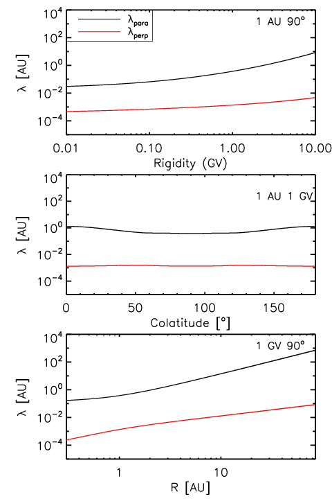
Figure 5 shows scenarios of mean free paths as a function of rigidity (top panel), polar angle (second panel), and radial distance (bottom panel). Interplanetary conditions are the same as that in Figure 2, and nT. The parallel mean free path shows stronger rigidity dependence when the rigidity increases, and is larger in the polar region as have been shown in the first and second panels. At lower energy, i.e., when energy is lower than about 3 GV, the parallel mean free path shows the expected dependence, but at higher energy the model gives a dependence. The perpendicular mean free path is relatively flat as a function of rigidity and colatitude. As has been shown in the bottom panel, the parallel and perpendicular mean free paths show a gradual increase with the radial distance.
II.6 Heliospheric boundary
Voyager 1 crossed the heliopause at AU in August 2012 and has reached the very local interstellar medium, Zhang et al. [106] believed that the solar modulation boundary is located a fraction of an AU beyond the heliopause. Therefore, the very local interstellar [76, 97, LIS, e.g.,] spectrum of GCRs could be used as the input spectrum in our modulation model. However, in our model, we set the outer boundary at a smaller solar distance AU, for simplicity purpose, so that we do not include the termination shock acceleration of GCRs and other complicated phenomenon in outer heliosphere. Furthermore, to keep solar distance not too large could make sure the diffusion model NLGCE-F always valid in this work. In addition, we assume the GCR source at AU as
| (42) |
where is a constant determined later and by following Zhang [105].
III Numerical Methods
To solve the Parker transport equation, we make use of the time-backward Markov stochastic process method proposed by Zhang [105]. For a pseudo-particle in position and momentum , the stochastic differential equations equivalent to Equation (1) have the form [105, 69, 90, 48]
| (43) |
with , the Ito processes [105], the backward time and satisfy a Wiener process given by the standard normal distribution [69, 90]. For the modified Parker HMF used in this work, the matrix components are given by Pei et al. [69] [48, see also],
| (44) | |||||
| (45) | |||||
| (46) | |||||
| (47) | |||||
| (48) | |||||
| (49) | |||||
| (50) |
and the components of vector are given as follows,
| (51) | |||||
| (52) | |||||
| (53) | |||||
| (54) |
Therefore the statistical differential equations can be written as
| (55) | |||||
| (56) | |||||
| (57) | |||||
| (58) |
Note that the diffusion tensor in Equations (55-58) are elements of the symmetric diffusion tensor in spherical coordinates. According to Burger et al. [21] elements of in spherical coordinates for the modified Parker HMF are written as
| (59) | |||||
| (60) | |||||
| (61) | |||||
| (62) | |||||
| (63) | |||||
| (64) |
with and , where is the HMF winding angle.
In our modulation model we use the time-delayed interplanetary conditions at radius related to the states at the source surface at some earlier time, and the heliosphere is considered dynamic due to the solar activities.
IV Modeling Results
In our GCR modulation model we only need four input parameters which can be obtained from the observations at AU, i.e., the heliospheric current sheet tilt angle, the solar wind speed, the magnitude of background magnetic field , and the magnetic turbulence magnitude . Figure 6 shows the computed and observed proton spectra for four Carrington rotations in November 2006, December 2007, December 2008, and December 2009 with colors cyan, purple, red, and blue, respectively. Circles means observations of PAMELA, numerical results of modulation modeling are shown as solid lines. The GCR source at AU is represented by the black line with the constant in Equation (42), and magenta triangles mean Voyager 2 observations at 85 AU reported by Webber et al. [100]. The modulation results show good agreement with the observations of PAMELA.
V Discussion and Conclusions
In this work, we develop a numerical model to study the time-dependent modulation of cosmic rays in recent solar minimum with PAMELA observations. We use the time-backward Markov stochastic process method [105] to numerically solve the Parker transport equation. In our GCR modulation model, all the parameters are obtained from the observations of OMNI. We get galactic proton spectra varying as a function of time during the recent solar minimum, which are consistent with the observations of PAMELA.
As the Parker HMF provides a low magnitude in the polar regions at large radial distance, we adopt the modified Parker HMF according to Jokipii & Kota [46], which can help to avoid the traditional Parker HMF’s problem that the drift speed of GCRs in polar regions are too large. Considering the dynamic phenomena of heliosphere with the solar wind flow from source surface to any solar distance, we use the input parameters observed near the Earth in the earlier time with a typical solar wind speed AU/day. It is noted that this will divide the heliosphere into slices and introduce an additional radial dependence in the HMF magnitude, i.e., . In the region between two slices of plasma the HMF is not divergence free, but in each step of the numerical solution of the TPE Equation (1), we always keep inside one slice of plasma. In addition, we set the outer boundary at a smaller solar distance AU, for simplicity purpose, so that we do not include the termination shock acceleration of GCRs and other complicated phenomenon in outer heliosphere. The GCR source spectrum we use is consistent with the observations of Voyager 2 at 85 AU reported by Webber et al. [100]. Furthermore, by keeping solar distance not too large we can make sure the diffusion model NLGCE-F always valid in this work.
The knowledge of transport of magnetic turbulence throughout the heliosphere is very important to determine the diffusion coefficients. According to previous studies [104, 21, 28, 63, 93, 71, e.g., ], we use a model for magnetic turbulence magnitude with Equation (32), i.e., , in which the latitudinal dependence is assumed from the observations of Ulysses, and the expression of for the radial dependence is chosen as a function of the heliospheric current sheet tilt angle with Equation (33). We show that the new turbulence magnitude model with Equations (32) and (33), denoted as TRST model, agrees well with the Ulysses, Voyager 1, and Voyager 2 observations. In addition, we assume two-component model of turbulence in solar wind. For simplicity purpose, we only suppose the magnetic turbulence magnitude is varying.
We use the new diffusion model NLGCE-F from Qin & Zhang [79] which was obtained by fitting the numerical solution from the non-linear parallel and perpendicular diffusion with polynomials. The using of the diffusion model NLGCE-F helps us to get more accurate diffusion coefficients without consuming lots of computing resources. For the drift coefficient, turbulence can provide the suppression [44, 33, 35, 25, 87, 60, 95, see, e.g., ]. The reduction of drift effects is complicated to be used self-consistently [13, 24, 95, see, e.g.,] or in Ad hoc form [23, 72, 98, 64, see, e.g.,] in modulation works. It is far from complete to understand the effects of turbulence on CR drifts. Therefore, in this work, we use the weak scattering drift coefficient for simplicity purpose.
In the future, we plan to use the modulation model established in this paper to study the 11 and 22 year modulation of GCRs in the inner heliosphere [57, 84, e.g.,]. If our model works well, we can reproduce the GCR observations by Ulysses, Voyager 1, and Voyager 2 with long period of time. Otherwise, we need to improve our modulation model. Firstly, we could improve the turbulence model by modifying the magnitude model and applying more realistic models for transport of turbulence geometry. Secondly, we could use a more self-consistent dynamic heliosphere model, e.g., a model from MHD simulation. Thirdly, we could include termination shock in the model to study the realistic boundary effects. Fourthly, the GCR source spectrum could be improved. Fifthly, the drift suppression from turbulence could be included.
References
- [1] Adhikari, L., Zank, G. P., Bruno, R., et al. 2015, ApJ, 805, 63
- [2] Adhikari, L., Zank, G. P., Hunana, P., et al. 2017, ApJ, 841, 85
- [3] Adriani, O., Barbarino, G. C., Bazilevskaya, G. A., et al. 2011a, Physical Review Letters, 106, 201101
- [4] Adriani, O., Barbarino, G. C., Bazilevskaya, G. A., et al. 2011b, Science, 332, 69
- [5] Adriani, O., Barbarino, G. C., Bazilevskaya, G. A., et al. 2013a, Physical Review Letters, 111, 081102
- [6] Adriani, O., Barbarino, G. C., Bazilevskaya, G. A., et al. 2013b, ApJ, 765, 91
- [7] Adriani, O., Barbarino, G. C., Bazilevskaya, G. A., et al. 2014a, ApJ, 791, 93
- [8] Adriani, O., Barbarino, G. C., Bazilevskaya, G. A., et al. 2014b, Phys. Rep., 544, 323
- [9] Adriani, O., Barbarino, G. C., Bazilevskaya, G. A., et al. 2015, ApJ, 810, 142
- [10] Ahluwalia, H. S., Lopate, C., Ygbuhay, R. C., & Duldig, M. L. 2010, Advances in Space Research, 46, 934
- [11] Ahluwalia, H. S., & Ygbuhay, R. C. 2011, Advances in Space Research, 48, 61
- [12] Balogh, A., Smith, E. J., Tsurutani, B. T., et al. 1995, Science, 268, 1007
- [13] Bieber, J. W., & Matthaeus, W. H. 1997, ApJ, 485, 655
- [14] Bieber, J. W., Matthaeus, W. H., Smith, C. W., et al. 1994, ApJ, 420, 294
- [15] Bisschoff, D., & Potgieter, M. S. 2016, Ap&SS, 361, 48
- [16] Bobik, P., Boella, G., Boschini, M. J., et al. 2012, ApJ, 745, 132
- [17] Bobik, P., Boella, G., Boschini, M. J., et al. 2013, Advances in Astronomy, 2013, 793072
- [18] Boschini, M. J., Della Torre, S., Gervasi, M., La Vacca, G., & Rancoita, P. G. 2017, ArXiv e-prints, arXiv:1704.03733
- [19] Breech, B., Matthaeus, W. H., Minnie, J., et al. 2008, Journal of Geophysical Research (Space Physics), 113, A08105
- [20] Burger, R. A. 2012, ApJ, 760, 60
- [21] Burger, R. A., Krüger, T. P. J., Hitge, M., & Engelbrecht, N. E. 2008, ApJ, 674, 511
- [22] Burger, R. A., & Potgieter, M. S. 1989, ApJ, 339, 501
- [23] Burger, R. A., Potgieter, M. S., & Heber, B. 2000, J. Geophys. Res., 105, 27447
- [24] Burger, R. A., & Visser, D. J. 2010, ApJ, 725, 1366
- [25] Candia, J., & Roulet, E. 2004, J. Cosmology Astropart. Phys, 10, 007
- [26] de Simone, N., di Felice, V., Gieseler, J., et al. 2011, Astrophysics and Space Sciences Transactions, 7, 425
- [27] Di Felice, V., Munini, R., Vos, E. E., & Potgieter, M. S. 2017, ApJ, 834, 89
- [28] Effenberger, F., Fichtner, H., Scherer, K., et al. 2012, ApJ, 750, 108
- [29] Engelbrecht, N. E., & Burger, R. A. 2013a, ApJ, 772, 46
- [30] Engelbrecht, N. E., & Burger, R. A. 2013b, ApJ, 779, 158
- [31] Engelbrecht, N. E., & Burger, R. A. 2015, Advances in Space Research, 55, 390
- [32] Ferreira, S. E. S., & Potgieter, M. S. 2004, ApJ, 603, 744
- [33] Fisk, L. A., & Schwadron, N. A. 1995, J. Geophys. Res., 100, 7865
- [34] Galper, A. M., Sparvoli, R., Adriani, O., et al. 2017, in Journal of Physics Conference Series, Vol. 798, Journal of Physics Conference Series, 012033
- [35] Giacalone, J., & Jokipii, J. R. 1999, ApJ, 520, 204
- [36] Gieseler, J., & Heber, B. 2016, A&A, 589, A32
- [37] Gleeson, L. J., & Axford, W. I. 1968, ApJ, 154, 1011
- [38] Gleeson, L. J., & Urch, I. H. 1971, Ap&SS, 11, 288
- [39] Guo, X., & Florinski, V. 2014, Journal of Geophysical Research (Space Physics), 119, 2411
- [40] Guo, X., & Florinski, V. 2016, ApJ, 826, 65
- [41] Heber, B., & Potgieter, M. S. 2006, Space Sci. Rev., 127, 117
- [42] Isenberg, P. A., Smith, C. W., Matthaeus, W. H., & Richardson, J. D. 2010, ApJ, 719, 716
- [43] Jokipii, J. R. 1966, ApJ, 146, 480
- [44] Jokipii, J. R. 1993, International Cosmic Ray Conference, 3, 497
- [45] Jokipii, J. R., & Kopriva, D. A. 1979, ApJ, 234, 384
- [46] Jokipii, J. R., & Kota, J. 1989, Geophys. Res. Lett., 16, 1
- [47] Jokipii, J. R., Levy, E. H., & Hubbard, W. B. 1977, ApJ, 213, 861
- [48] Kopp, A., Büsching, I., Strauss, R. D., & Potgieter, M. S. 2012, Computer Physics Communications, 183, 530
- [49] Kota, J., & Jokipii, J. R. 1983, ApJ, 265, 573
- [50] Langner, U. W. 2004, PhD thesis, Potchestroom University
- [51] Manuel, R., Ferreira, S. E. S., & Potgieter, M. S. 2014, Sol. Phys., 289, 2207
- [52] Manuel, R., Ferreira, S. E. S., Potgieter, M. S., Strauss, R. D., & Engelbrecht, N. E. 2011, Advances in Space Research, 47, 1529
- [53] Matthaeus, W. H., Goldstein, M. L., & Roberts, D. A. 1990, J. Geophys. Res., 95, 20673
- [54] Matthaeus, W. H., Qin, G., Bieber, J. W., & Zank, G. P. 2003, ApJ, 590, L53
- [55] McComas, D. J., Ebert, R. W., Elliott, H. A., et al. 2008, Geophys. Res. Lett., 35, L18103
- [56] McComas, D. J., Elliott, H. A., Gosling, J. T., et al. 2002, Geophys. Res. Lett., 29, 4
- [57] McDonald, F. B. 1998, Space Sci. Rev., 83, 33
- [58] Mewaldt, R. A. 2013, Space Sci. Rev., 176, 365
- [59] Mewaldt, R. A., Davis, A. J., Lave, K. A., et al. 2010, ApJ, 723, L1
- [60] Minnie, J., Bieber, J. W., Matthaeus, W. H., & Burger, R. A. 2007, ApJ, 670, 1149
- [61] Mori, N., Adriani, O., Barbarino, G., et al. 2015, Nuclear and Particle Physics Proceedings, 265, 242
- [62] Ndiitwani, D. C., Potgieter, M. S., Manuel, R., & Ferreira, S. E. S. 2013, in Proceedings, 33rd International Cosmic Ray Conference (ICRC2013), ICRC2013–0187
- [63] Ngobeni, M. D., & Potgieter, M. S. 2014, Advances in Space Research, 53, 1634
- [64] Nndanganeni, R. R., & Potgieter, M. S. 2016, Advances in Space Research, 58, 453
- [65] Oughton, S., Matthaeus, W. H., Smith, C. W., Breech, B., & Isenberg, P. A. 2011, Journal of Geophysical Research (Space Physics), 116, A08105
- [66] Parker, E. N. 1958, ApJ, 128, 664
- [67] Parker, E. N. 1965, Planet. Space Sci., 13, 9
- [68] Pei, C., Bieber, J. W., Breech, B., et al. 2010a, Journal of Geophysical Research (Space Physics), 115, A03103
- [69] Pei, C., Bieber, J. W., Burger, R. A., & Clem, J. 2010b, Journal of Geophysical Research (Space Physics), 115, A12107
- [70] Pei, C., Bieber, J. W., Burger, R. A., & Clem, J. 2012, ApJ, 744, 170
- [71] Perri, S., & Balogh, A. 2010, Geophys. Res. Lett., 37, L17102
- [72] Potgieter, M. 2013, Living Reviews in Solar Physics, 10, arXiv:1306.4421
- [73] Potgieter, M. S. 2000, J. Geophys. Res., 105, 18295
- [74] Potgieter, M. S., Burger, R. A., & Ferreira, S. E. S. 2001, Space Sci. Rev., 97, 295
- [75] Potgieter, M. S., Mwiinga, N., Ferreira, S. E. S., Manuel, R., & Ndiitwani, D. C. 2013, Journal of Advanced Research, 4, 259
- [76] Potgieter, M. S., Vos, E. E., Boezio, M., et al. 2014, Sol. Phys., 289, 391
- [77] Potgieter, M. S., Vos, E. E., Munini, R., Boezio, M., & Di Felice, V. 2015, ApJ, 810, 141
- [78] Qin, G. 2007, ApJ, 656, 217
- [79] Qin, G., & Zhang, L.-H. 2014, ApJ, 787, 12
- [80] Raath, J. L., Potgieter, M. S., Strauss, R. D., & Kopp, A. 2016, Advances in Space Research, 57, 1965
- [81] Raath, J. L., Strauss, R. D., & Potgieter, M. S. 2015, Ap&SS, 360, 24
- [82] Schrijver, C. J., Livingston, W. C., Woods, T. N., & Mewaldt, R. A. 2011, Geophys. Res. Lett., 38, L06701
- [83] Sheeley, N. R., Wang, Y.-M., Hawley, S. H., et al. 1997, ApJ, 484, 472
- [84] Shen, Z.-N., & Qin, G. 2016, Journal of Geophysical Research (Space Physics), 121, 10
- [85] Smith, C. W., Isenberg, P. A., Matthaeus, W. H., & Richardson, J. D. 2006, ApJ, 638, 508
- [86] Smith, E. J., & Balogh, A. 2008, Geophys. Res. Lett., 35, L22103
- [87] Stawicki, O. 2005, ApJ, 624, 178
- [88] Stone, E. C., Cummings, A. C., McDonald, F. B., et al. 2013, Science, 341, 150
- [89] Strauss, R. D., & Potgieter, M. S. 2010, Journal of Geophysical Research (Space Physics), 115, A12111
- [90] Strauss, R. D., Potgieter, M. S., Büsching, I., & Kopp, A. 2011a, ApJ, 735, 83
- [91] Strauss, R. D., Potgieter, M. S., Büsching, I., & Kopp, A. 2012, Ap&SS, 339, 223
- [92] Strauss, R. D., Potgieter, M. S., & Ferreira, S. E. S. 2011b, Advances in Space Research, 48, 65
- [93] Strauss, R. D. T., Dresing, N., & Engelbrecht, N. E. 2017, The Astrophysical Journal, 837, 43
- [94] Svalgaard, L., Cliver, E. W., & Kamide, Y. 2005, in Astronomical Society of the Pacific Conference Series, Vol. 346, Large-scale Structures and their Role in Solar Activity, ed. K. Sankarasubramanian, M. Penn, & A. Pevtsov, 401
- [95] Tautz, R. C., & Shalchi, A. 2012, ApJ, 744, 125
- [96] Usoskin, I. G., Bazilevskaya, G. A., & Kovaltsov, G. A. 2011, Journal of Geophysical Research (Space Physics), 116, A02104
- [97] Vos, E. E., & Potgieter, M. S. 2015, ApJ, 815, 119
- [98] Vos, E. E., & Potgieter, M. S. 2016, Sol. Phys., 291, 2181
- [99] Vourlidas, A., Howard, R. A., Esfandiari, E., et al. 2010, ApJ, 722, 1522
- [100] Webber, W. R., Cummings, A. C., McDonald, F. B., et al. 2008, Journal of Geophysical Research (Space Physics), 113, A10108
- [101] Webber, W. R., & McDonald, F. B. 2013, Geophys. Res. Lett., 40, 1665
- [102] Zank, G. P., Adhikari, L., Hunana, P., et al. 2017, ApJ, 835, 147
- [103] Zank, G. P., Dosch, A., Hunana, P., et al. 2012, ApJ, 745, 35
- [104] Zank, G. P., Matthaeus, W. H., & Smith, C. W. 1996, J. Geophys. Res., 101, 17093
- [105] Zhang, M. 1999, ApJ, 513, 409
- [106] Zhang, M., Luo, X., & Pogorelov, N. 2015, Physics of Plasmas, 22, doi:http://dx.doi.org/10.1063/1.4928945
- [107] Zhao, L.-L., Qin, G., Zhang, M., & Heber, B. 2014, Journal of Geophysical Research (Space Physics), 119, 1493
- [108] Zurbuchen, T. H. 2007, ARA&A, 45, 297