Coherent Transport in Photonic Lattices:
A Survey of Recent Analytic Results

This paper reviews recent analytic results on the perfect transfer and fractional revival of states or excitations in photonic lattices using a general method that also applies to spin chains, tight-binding Hamiltonians, etc. Controlling the evolution of quantum states in devices is of high relevance in areas such as quantum information. With an eye to offering a clean basis for experimental testing, it is also quite practical to look for exact analytical descriptions of such systems. Another objective is to minimize the need for external controls to achieve given tasks, in this respect a key idea is to construct devices whose dynamics will yield on its own the desired effect leaving only the input/output operations as external interactions.

A basic task is the transportation of quantum states from one location to another. Ideally one wishes to have perfect state transfer (PST) whereby a quantum state at an initial position is found with probability $1$ at the final destination. While there has been seminal work on optical Bloch oscillations in waveguide arrays, see for instance [13, 25, 40], this review focuses on coherent transport in spin-inspired photonic lattices. Since it has been suggested that spin chains [4] with properly modulated couplings [1, 10] could move a qubit from end-to-end with probability $1$ in a given time, there has been enormous interest in this question and indeed various analytic models have been found [6, 26, 34, 46, 47, 49, 50, 51]. See [5, 29, 38] for reviews. Remarkably experimental verifications have been offered [3, 7, 39] for the simplest (Krawtchouk) model with PST by using arrays of evanescently coupled waveguides [12, 33, 36]. These can be pictured as a set of optical fibers stacked side by side in a plane. The point is that in the nearest-neighbour approximation, the equations of coupled mode theory describing the propagation of a single photon in waveguide arrays are mathematically identical to those governing the one-excitation dynamics of a certain spin chain with non-uniform couplings. Each qubit is represented by a single waveguide and the presence or absence of a photon in a waveguide corresponds to the $\rvert 1\rangle$ or $\rvert 0\rangle$ state of the qubit at the corresponding site. The evolution time $t$ of the spin chain is identified with the propagation distance $z$ along the waveguides. Therefore PST is tantamount to finding in the last waveguide after a distance $Z_{\rm PST}$, the photon initially inserted (at $z=0$) in the first fiber of the array¹¹ 1 Strictly speaking in the photonic lattice realizations, one is producing an excitation transfer. In a spin chain, a state, i.e., an arbitrary combination of spin up and down will be transported. This is modeled in [7] in an optical settings by encoding a state in polarizations.. The required couplings between the waveguides are engineered by adjusting the distances so that they match the theoretical values. The analysis that underscores the design of the spin chains/photonic lattices with PST shows that the couplings and local magnetic fields/propagation constants correspond to the recurrence coefficients of orthogonal polynomials that are naturally associated to these systems. The analytic models in fact correspond to orthogonal polynomials that have been fully characterized [32] and they are thus referred to by the name of the polynomials that are attached to them. We have already hinted at that above when we mentioned the Krawtchouk model.

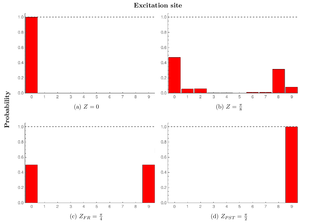
It has more recently been observed that spin chains and waveguide arrays can also exhibit another phenomenon called fractional revival (FR) which is of significant interest as it relates to entanglement generation. Fractional revival [15, 29] occurs when an initial wavepacket evolves so as to reproduce itself periodically at certain locations [2, 8, 16, 20, 31, 43]. We shall here be interested in FR at two sites along a spin chain whereby a spin up initially at one end will evolve so as to have, after some FR time, a non-zero probability amplitude only at both ends of the chain. In the photonic picture, this means that the electromagnetic field amplitude is non-zero only in the first and last waveguide. Using the qubit correspondence, this means that after propagating a distance $Z_{\rm FR}$ the state $\rvert 10\dots 0\rangle$ has evolved into the entangled state $\alpha\rvert 10\dots 0\rangle+\beta\rvert 0\dots 01\rangle$.

Interestingly the exploration of the conditions for this FR at two sites has led to the discovery of a new family of orthogonal polynomials [51], named the para-Krawtchouk polynomials, that have been completely characterized and this has hence provided a model which is the paradigm example of a device with FR at the two ends [21]. The FR properties of other analytic models known to have PST have recently been examined; these results will be succinctly reported here. It would of course be quite interesting to realize FR experimentally in photonic lattices in a way similar to what was done for PST.

When using photonic lattices, the restriction to nearest-neighbour (NN) couplings is clearly an approximation. As a mean to explore the validity of this simplification and to determine if new phenomenology can arise when the approximation is improved [28, 48], an analytic model with next-to-nearest couplings and based on the simplest Krawtchouk model has been constructed [11]. It will be discussed towards the end.

In a nutshell the goal of this short review article is: $1)$ to summarize how orthogonal polynomials intervene in the characterization of photonic lattices with FR and PST; $2)$ to go over a selection of recent results in this respect and $3)$ to offer a compact catalog of analytic models with these properties.

The outline of the paper is as follows. The connection between photon propagation in waveguide arrays and orthogonal polynomials is set up in Section 2. The special conditions for FR and PST in these ensembles of waveguides when the NN approximation is made are given in Section 3. How the specifications of the lattices are determined from these conditions using orthogonal polynomials is briefly indicated in Section 4. Section 5 which is the bulk of the paper goes over a number of analytic models and discusses their FR and PST properties. Some material in this section is original. Section 6 describes one analytic model with next-to-nearest neighbour couplings and comments on extensions and generalizations. A short conclusion completes the paper.

Spin chains and photonic lattices are usefully analyzed with the help of orthogonal polynomials (see for instance [17, 29, 41, 44, 50]). Let us consider an array of $(N+1)$ evanescently coupled optical waveguides. Denote by $z$ the propagation distance and by $E_{n}$ the modal field amplitude in the $n$^th waveguide. In the nearest-neighbour approximation of coupled mode theory [24, 45], the propagation is governed by

$B_{n}$ is the propagation constant in the $n$^th waveguide and $J_{n+1}$, a positive real number, is the evanescent coupling strength between the waveguides $n$ and $n+1$. This $J_{n+1}$ is (approximately) given by

where $d_{n,n+1}$ is the distance between the $n$^th and ($n+1$)^th waveguides and $A$, $C$ are measurable quantities that specify the array. Upon introducing the natural basis of $\mathbb{C}^{N+1}$ made out of the vectors

with 1 in the $n$^th position and positing

one can rewrite (2.1) in the form

where $J$ is the operator defined by

again with $J_{0}=J_{N+1}=0$. It thus follows that

where in the basis $\{\rvert n\rangle\}$, $J$ is the tridiagonal matrix

The Jacobi matrix $J$ is Hermitian and has non-degenerate eigenvalues $\lambda_{s}$, $s=0,1,\dots,N$ when its entries are non-negative. Let us denote the eigenvectors of $J$ by $\rvert\lambda_{s}\rangle$:

We shall now indicate how orthogonal polynomials are naturally associated to the dynamics. This simply follows from the fact that Jacobi matrices are diagonalized by orthogonal polynomials. Consider the expansion of the eigenbasis $\{\rvert\lambda_{s}\rangle\}$ in term of the natural basis $\{\rvert n\rangle\}$:

Acting on both sides with $J$, we get

and since the natural basis is orthonormal, we have

Taking $W_{s,n}$ in the form

we see that the coefficients $\chi_{n}(x)$, $n=0,1,\dots,N$, constitute an orthogonal polynomial set owing to the fact that they satisfy the three term recurrence relation

with the initial condition $\chi_{-1}(x)=0$. Since both bases are orthonormal, $\langle s\rvert s^{\prime}\rangle=\delta_{ss^{\prime}}$ and $\langle n\rvert m\rangle=\delta_{nm}$ it follows that the matrix ($W_{s,n}$) is orthogonal

The reverse expansion is thus given by

and one explicitly recovers from $\langle n\rvert m\rangle=\delta_{nm}$ that the functions $\chi_{n}(\lambda_{s})$ are normalized orthogonal polynomials in the discrete variable $\lambda_{s}$. The orthogonality relation reads

with $w_{s}=W_{s0}^{2}$ playing the role of the weight.

We can define the monic polynomials $P_{n}(x)$

Furthermore the characteristic polynomial $P_{N+1}(x)$

is manifestly orthogonal to the polynomials $\chi_{n}(x)$, $n=0,\dots,N$. From the general theory of orthogonal polynomials, it is known that [9] the discrete weights $w_{s}$ can be written in the form

where

and where $P^{\prime}_{N+1}(x)$ stands for the derivative of $P_{N+1}(x)$. If one takes the eigenvalues in increasing order,

it is easy to see that

To achieve PST and FR, some conditions must be respected. These, in fact, will only depend on the spectrum of $J$. PST will be achieved if a photon initially in the waveguide $0$ will be found in the waveguide $N$ after a propagation distance $Z_{\rm PST}$, in other words PST will be observed if

with $\phi$ an arbitrary phase.

Using the expansion (2.3) of the natural basis into the eigenbasis and remembering that $\chi_{0}(x)=1$, one sees that (3.1) implies

This shows that $\chi_{N}(\lambda_{s})$ is a phase, but since it is real we must have

Owing to the fact that the zeros of $\chi_{N}(x)$ must interlace the zeros, $\lambda_{s}$, of $P_{N+1}(x)$, the sign of $\chi_{N}(\lambda_{s})$ must alternate, i.e., $\chi_{N}(\lambda_{s})\propto(-1)^{s}$. Now since $w_{s}$ as given by (2.4) must be positive, in view of (2.5), we see that

As shown in [29], this condition is tantamount to the matrix $J$ being symmetric with respect to the anti-diagonal, i.e., to the relations

The condition (3.3) or equivalently (3.4) is thus necessary for the occurrence of PST.

Making use of this necessary condition in (3.2) one finds that PST will take place if

This will be satisfied if

where $L_{s}$ is a sequence of integers that may depend on $s$.

It follows from (3.5) that the difference between 2 successive eigenvalues is given by

where $M_{s}$ is an odd integer.

Together (3.4) and (3.6) are necessary and sufficient for PST. As announced, these are conditions on the spectrum of $J$.

Let us now turn to FR in the two external waveguides. This will occur if there is a distance $Z_{\rm FR}$ at which the only non-zero amplitudes are $E_{0}(Z_{\rm FR})$ and $E_{N}(Z_{\rm FR})$. In this case we shall have

with the normalization condition

When this is so, the wavepacket initially localized in the waveguide $0$ is revived in the waveguide $0$ and $N$. In the special case

we have an analog of the maximally entangled state $\rvert E\rangle=\frac{E_{0}(0)}{\sqrt{2}}(\rvert 10\dots 0\rangle+\rvert 00\dots 1\rangle)$ where the vectors $\rvert 1\rangle$, $\rvert 0\rangle$ denote the presence ($\rvert 1\rangle$) or the absence ($\rvert 0\rangle$) of a photon in the waveguide. One also sees that PST is a special case of FR with

As for PST, the relation (3.7) can be translated into a spectral condition by using the expansion (2.3). This leads to

In the following we shall look for the occurrence of FR in systems with mirror symmetry (3.4). We shall thus assume that the necessary condition (3.3) for PST is satisfied. As a result (3.8) will read

where we have factored out the phase $e^{i\phi}$ of $\mu$ implying that $\mu=e^{i\phi}\mu^{\prime}$ with $\mu^{\prime}$ real and $\nu=e^{i\phi}\nu^{\prime}$. For consistency, the norm of ($\mu^{\prime}+(-1)^{N+s}\nu^{\prime}$) must be $1$ and with $\mu^{\prime}$ real this requires $\nu^{\prime}$ to be purely imaginary. Since $|\mu|^{2}+|\nu|^{2}=1$, we may thus take the following parametrization

Observe then that PST ($\mu=0$) corresponds to $\theta=\frac{\pi}{2}$. As in the case for PST, condition (3.9) can be seen to imply restrictions on successive eigenvalues:

where $L^{(i)}_{s}$ are arbitrary sequences of integers that depend on $s$.

FR will occur if those conditions are respected for all eigenvalues of the spectrum. Note that, as shown in [21], in this mirror-symmetric situation, FR also occurs between symmetrically positioned sites say between $\rvert n\rangle$ and $\rvert N-n\rangle$.

The engineering of photonic lattices with FR and PST involves an inverse spectral problem, as first discussed in [27]. Given a set of $\{\lambda_{s}\}$ that satisfy the FR/PST conditions, we must find the mirror-symmetric matrix $J$ formed out of the coupling and propagation constants that has the $\{\lambda_{s}\}$ for eigenvalues. This is done by constructing the orthogonal polynomials associated to the problem whose recurrence coefficients will provide the characteristics of the array that we are looking for. Once these have been obtained, it is a matter of creating appropriately the waveguides and of choosing the distances between them to make the specifications of the lattice match those prescribed theoretically.

Let us briefly recall how this inverse spectral problem is solved from the construction of the associated orthogonal polynomials. First, observe that the condition $\chi_{N}(\lambda_{s})=(-1)^{N+s}$ fixes the values of a polynomial of degree $N$ at $N+1$ points and thereby completely determines $\chi_{N}(x)$. This polynomial can be explicitly constructed using the Lagrange interpolation polynomials:

Here $\mathcal{L}_{s}$ is the standard Lagrange polynomial

where the ^′ stands for $i\neq s$.

The monic polynomial $P_{N}(x)$ is then obtained by dividing $\chi_{N}(x)$ by the coefficient of $x^{N}$. The spectral data $\{\lambda_{s}\}$ provides another member of the set of orthogonal polynomials, namely, the characteristic polynomial $P_{N+1}(x)=(x-\lambda_{0})\cdots(x-\lambda_{N})$. The recurrence relation for the monic polynomials $P_{n}(x)=J_{1}\cdots J_{n}\chi_{n}(x)$ is

with $U_{n}=J_{n}^{2}$. For all these polynomials $P_{n}(x)$, the coefficients of the leading monomial $x^{n}$ is $1$.

We thus have

We know $P_{N+1}$ and $P_{N}$. If we look at (4.1) degree by degree, we see that the terms in $x^{N+1}$ are equal. Then the coefficient of $x^{N}$ in $P_{N+1}$ gives $-B_{N}$. Now the coefficients of $x^{N-1}$ in $P_{N+1}(x)-(x-B_{N})P_{N}(x)$ gives $-J_{N}^{2}$ and at this point we know $B_{N}$, $J_{N}^{2}$ and $P_{N-1}(x)$. We can then iterate to find $B_{N-1}$, $J_{N-1}^{2}$ and $P_{N-2}(x)$ and so on. In the end the mirror-symmetric matrix $J$ is fully characterized and hence provides all the couplings $J_{n}$ and propagation constants $B_{n}$ for $n=0,\dots,N$.

While the algorithm described above is conceptually straightforward it might not be the most efficient to obtain the parameters numerically. Another method is given in Gladwell [22]; the approach described in [19] based on persymmetric polynomials is also generally faster.

In a number of cases, spectra that satisfy (3.6) and (3.10) have been found to correspond to orthogonal polynomials that can be fully characterized and this has therefore led to models that can be described analytically. These arrays are often referred to by the name of the orthogonal polynomials associated to them and turn out to be most useful. They have first been identified for their PST properties. In the following we shall go over many of these systems. We shall give in each case the corresponding spectrum $\{\lambda_{s}\}$ and provide the couplings $J_{n}$ and propagation constants $B_{n}$ that the algorithm described in Section 4 gives. We shall indicate what the FR and PST conditions entail. For FR we shall provide the mixing angles $\theta$ that are possible as well as the distances $Z_{\rm FR}$ at which this FR occurs. We shall also record the restrictions that must be imposed for PST to happen also. To allow for an adjustment of the reference strength of the couplings we shall introduce a parameter $\beta$ as a global factor in the spectra: $\lambda_{s}\rightarrow\beta\lambda_{s}$.

References

- [1] Albanese C., Christandl M., Datta N., Ekert A., Mirror inversion of quantum states in linear registers, Phys. Rev. Lett. 93 (2004), 230502, 4 pages, quant-ph/0405029.
- [2] Banchi L., Compagno E., Bose S., Perfect wave-packet splitting and reconstruction in a one-dimensional lattice, Phys. Rev. A 91 (2015), 052323, 8 pages, arXiv:1502.03061.
- [3] Bellec M., Nikolopoulos G.M., Tzortzakis S., Faithful communication Hamiltonian in photonic lattices, Opt. Lett. 37 (2012), 4504–4506, arXiv:1210.1009.
- [4] Bose S., Quantum communication through an unmodulated spin chain, Phys. Rev. Lett. 91 (2003), 207901, 4 pages, quant-ph/0212041.
- [5] Bose S., Quantum communication through spin chain dynamics: an introductory overview, Contemp. Phys. 48 (2007), 13–30, arXiv:0802.1224.
- [6] Chakrabarti R., Van der Jeugt J., Quantum communication through a spin chain with interaction determined by a Jacobi matrix, J. Phys. A: Math. Theor. 43 (2010), 085302, 20 pages, arXiv:0912.0837.
- [7] Chapman R.J., Santandrea M., Huang Z., Corrielli G., Crespi A., Yung M.-H., Osellame R., Peruzzo A., Experimental perfect state transfer of an entangled photonic qubit, Nature Comm. 7 (2016), 11339, 6 pages, arXiv:1603.00089.
- [8] Chen B., Song Z., Sun C.P., Fractional revivals of the quantum state in a tight-binding chain, Phys. Rev. A 75 (2007), 012113, 9 pages, quant-ph/0603033.
- [9] Chihara T.S., An introduction to orthogonal polynomials, Mathematics and its Applications, Vol. 13, Gordon and Breach Science Publishers, New York – London – Paris, 1978.
- [10] Christandl M., Datta N., Ekert A., Landahl A.J., Perfect state transfer in quantum spin networks, Phys. Rev. Lett. 92 (2004), 187902, 4 pages, quant-ph/0309131.
- [11] Christandl M., Vinet L., Zhedanov A., Analytic next-to-nearest neighbour XX models with perfect state transfer and fractional revival, arXiv:1607.02639.
- [12] Christodoulides D.N., Lederer F., Silberberg Y., Discretizing light behaviour in linear and nonlinear waveguide lattices, Nature 424 (2003), 817–823.
- [13] Corrielli G., Crespi A., Della Valle G., Longhi S., Osellame R., Fractional Bloch oscillations in photonic lattices, Nature Comm. 4 (2013), 11339, 6 pages, arXiv:1303.1958.
- [14] Coutinho G.M., State transfer on graphs, Ph.D. Thesis, University of Waterloo, 2014.
- [15] Dai L., Feng Y.P., Kwek L.-C., Engineering quantum cloning through maximal entanglement between boundary qubits in an open spin chain, J. Phys. A: Math. Theor. 43 (2010), 035302, 14 pages.
- [16] De Chiara G., Fazio R., Macchiavello C., Montangero S., Palma G.M., Quantum cloning in spin networks, Phys. Rev. A 70 (2004), 062308, 4 pages, quant-ph/0402071.
- [17] Efremidis N.K., Christodoulides D.N., Revivals in engineered waveguide arrays, Opt. Comm. 246 (2005), 345–356.
- [18] Genest V.X., Miki H., Vinet L., Zhedanov A., Spin lattices, state transfer, and bivariate Krawtchouk polynomials, Can. J. Phys. 93 (2015), 979–984, arXiv:1410.4703.
- [19] Genest V.X., Tsujimoto S., Vinet L., Zhedanov A., Persymmetric Jacobi matrices, isospectral deformations and orthogonal polynomials, J. Math. Anal. Appl. 450 (2017), 915–928, arXiv:1605.00708.
- [20] Genest V.X., Vinet L., Zhedanov A., Exact fractional revival in spin chains, Modern Phys. Lett. B 30 (2016), 1650315, 7 pages, arXiv:1506.08434.
- [21] Genest V.X., Vinet L., Zhedanov A., Quantum spin chains with fractional revival, Ann. Physics 371 (2016), 348–367, arXiv:1507.05919.
- [22] Gladwell G.M.L., Inverse problems in vibration, Solid Mechanics and its Applications, Vol. 119, 2nd ed., Kluwer Academic Publishers, Dordrecht, 2005.
- [23] Godsil C., State transfer on graphs, Discrete Math. 312 (2012), 129–147, arXiv:1102.4898.
- [24] Huang W.-P., Coupled-mode theory for optical waveguides: an overview, J. Opt. Soc. Amer. A 11 (1994), 963–983.
- [25] Iwanow R., May-Arrioja D.A., Christodoulides D.N., Stegeman G.I., Min Y., Sohler W., Discrete Talbot effect in waveguide arrays, Phys. Rev. Lett. 95 (2005), 053902, 4 pages.
- [26] Jafarov E.I., Van der Jeugt J., Quantum state transfer in spin chains with -deformed interaction terms, J. Phys. A: Math. Theor. 43 (2010), 405301, 18 pages, arXiv:1005.2912.
- [27] Karbach P., Stolze J., Spin chains as perfect quantum state mirrors, Phys. Rev. A 72 (2005), 030301, 4 pages, quant-ph/0501007.
- [28] Kay A., Perfect state transfer: beyond nearest-neighbor couplings, Phys. Rev. A 73 (2006), 032306, 7 pages, quant-ph/0509065.
- [29] Kay A., Perfect, efficient, state transfer and its application as a constructive tool, Int. J. Quantum Inform. 8 (2010), 641–676, arXiv:0903.4274.
- [30] Kay A., Generating quantum states through spin chain dynamics, New J. Phys. 19 (2017), 043019, 15 pages, arXiv:1609.01398.
- [31] Kay A., Tailoring spin chain dynamics for fractional revivals, Quantum 1 (2017), 24, 11 pages, arXiv:1609.01397.
- [32] Koekoek R., Lesky P.A., Swarttouw R.F., Hypergeometric orthogonal polynomials and their -analogues, Springer Monographs in Mathematics, Springer-Verlag, Berlin, 2010.
- [33] Lederer F., Stegeman G.I., Christodoulides D.N., Assanto G., Segev M., Silberberg Y., Discrete solitons in optics, Phys. Rep. 463 (2008), 1–126.
- [34] Lemay J.-M., Vinet L., Zhedanov A., An analytic spin chain model with fractional revival, J. Phys. A: Math. Theor. 49 (2016), 335302, 15 pages, arXiv:1509.08965.
- [35] Lemay J.-M., Vinet L., Zhedanov A., The para-Racah polynomials, J. Math. Anal. Appl. 438 (2016), 565–577, arXiv:1511.05215.
- [36] Longhi S., Quantum-optical analogies using photonic structures, Laser Photonics Rev. 3 (2009), 243–261.
- [37] Miki H., Tsujimoto S., Vinet L., Zhedanov A., Quantum-state transfer in a two-dimensional regular spin lattice of triangular shape, Phys. Rev. A 85 (2012), 062306, 4 pages, arXiv:1203.2128.
- [38] Nikolopoulos G.M., Jex I. (Editors), Quantum state transfer and network engineering, Quantum Science and Technology, Springer, Heidelberg, 2014.
- [39] Perez-Leija A., Keil R., Kay A., Moya-Cessa H., Nolte S., Kwek L.-C., Rodríguez-Lara B.M., Szameit A., Christodoulides D.N., Coherent quantum transport in photonic lattices, Phys. Rev. A 87 (2013), 012309, 8 pages, arXiv:1207.6080.
- [40] Peschel U., Pertsch T., Lederer F., Optical Bloch oscillations in waveguide arrays, Opt. Lett. 23 (1998), 1701–1703.
- [41] Petrovic J., Multiport waveguide couplers with periodic energy exchange, Opt. Lett. 40 (2015), 139–142.
- [42] Post S., Quantum perfect state transfer in a 2D lattice, Acta Appl. Math. 135 (2015), 209–224.
- [43] Robinett R.W., Quantum wave packet revivals, Phys. Rep. 392 (2004), 1–119, quant-ph/0401031.
- [44] Rodríguez-Lara B.M., Exact dynamics of finite Glauber–Fock photonic lattices, Phys. Rev. A 84 (2011), 053845, 6 pages, arXiv:1108.3004.
- [45] Rodríguez-Lara B.M., Soto-Eguibar F., Christodoulides D.N., Quantum optics as a tool for photonic lattice design, Phys. Scr. 90 (2015), 068014, 7 pages.
- [46] Shi T., Li Y., Song Z., Sun C.-P., Quantum-state transfer via the ferromagnetic chain in a spatially modulated field, Phys. Rev. A 71 (2005), 032309, 5 pages, quant-ph/0408152.
- [47] Stoilova N.I., Van der Jeugt J., An exactly solvable spin chain related to Hahn polynomials, SIGMA 7 (2011), 033, 13 pages, arXiv:1101.4469.
- [48] Szameit A., Pertsch T., Nolte S., Tünnermann A., Peschel U., Lederer F., Optical Bloch oscillations in general waveguide lattices, J. Opt. Soc. Amer. B 24 (2007), 2632–2639.
- [49] Vinet L., Zhedanov A., Dual-1 Hahn polynomials and perfect state transfer, J. Phys. Conf. Ser. 343 (2012), 012125, 10 pages, arXiv:1110.6477.
- [50] Vinet L., Zhedanov A., How to construct spin chains with perfect state transfer, Phys. Rev. A 85 (2012), 012323, 7 pages, arXiv:1110.6474.
- [51] Vinet L., Zhedanov A., Para-Krawtchouk polynomials on a bi-lattice and a quantum spin chain with perfect state transfer, J. Phys. A: Math. Theor. 45 (2012), 265304, 11 pages, arXiv:1110.6475.
- [52] Yung M.-H., Quantum speed limit for perfect state transfer in one dimension, Phys. Rev. A 74 (2006), 030303, 4 pages, quant-ph/0603179.