Diffusion in deterministic interacting lattice systems

Introduction.– Understanding out-of-equilibrium phenomena has been at the forefront of condensed matter physics of the last decade. Despite the efforts, we have only recently gained a considerable insight into the microscopic origins of the transport in interacting systems in terms of an emerging field of generalized hydrodynamics (GHD) [1, 2, 3, 4, 5, 6, 7, 8, 9, 10, 11]. While GHD provides a general framework to analytically deal with the ballistic transport, in particular in integrable systems, it lacks an extension which would enable us to study normal, diffusive transport. In this regard, there are only a few results on lower bounding the diffusion constant in terms of local, or bilocal conserved charges [12, 13].

Since the integrable systems are characterized by ballistically propagating excitations [14], the question of how the diffusion, which is usually related to microscopic chaos, arises in integrable, locally interacting, clean and deterministic (i.e. non-disordered and non-dissipative) systems is puzzling to say the least [15, 16, 17, 18, 19, 20]. A great deal of attention has been devoted to the study of inhomogeneous quench problems, where two chains in equilibrium with distinct temperatures or chemical potentials are joined together and then let to evolve under a homogeneous Hamiltonian [1, 2, 3, 4, 5, 6, 7, 8, 9, 21]. In such situations, non-equilibrium steady states typically emerge on ballistic lines $x=vt$. However, for systems exhibiting parity-like symmetries, with respect to which the initial quench state is symmetric and the current anti-symmetric, the ballistic transport channel may close and time-dependent DMRG simulations clearly indicate that the steady state arises along diffusive lines $x=\xi\sqrt{t}$ [15].

In this Letter we expound one possible general mechanism for diffusive behavior in interacting systems, which as we show on an example, is connected to the interplay between freely propagating neutral degrees of freedom and insulating behavior of charge carrying ones. The model in question is a simple, reversible cellular automaton, consisting of three types of particles: freely moving vacancies, and hard-core interacting positive and negative charges. Despite the integrability, obtaining the full time dependence is usually intractable, except for non-interacting systems. Typically this presents an insurmountable barrier for calculation of transport coefficients. In our model, however, we explicitly compute the time dependence of current time autocorrelation functions in separable equilibrium states, and solve the inhomogeneous quench problem with arbitrary initial charge density bias resulting in a universal diffusive error function scaling profile. Depending on the density of vacancies and the imbalance of positive and negative charge three different regimes are identified. The absence of vacancies renders the system insulating, while in a generic case of the charge imbalance the system exhibits ideal transport. The regime with a finite density of vacancies and without the charge imbalance is especially interesting, since it includes the maximum entropy state, and in this regime the model exhibits purely diffusive transport.

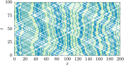
The model.– Consider a deterministic, reversible cellular automaton defined on the chain with  an even length of $n$ sites. Each site can be either vacant (state $\emptyset$), or occupied by a positively or negatively charged particle (state $+$ or $-$). The dynamics of the lattice configuration, ${\underline{s}}=(s_{1},\ldots,s_{n}),s_{x}\in\{\emptyset,+,-\}$, can be expressed in terms of a local two site mapping $\phi_{x,x+1}({\underline{s}})=(s_{1},s_{2},\dots,s^{\prime}_{x},s^{\prime}_{x+1},\dots,s_{n})$, where the updated elements $(s_{x}^{\prime},s_{x+1}^{\prime})$ are obtained from the initial ones $(s_{x},s_{x+1})$, by a self-inverse transformation

with $\alpha,\beta\in\{+,-\}$. The local process describes the elastic scattering of charged particles. The lattice configuration at time $t,$ ${\underline{s}}^{t}=\phi({\underline{s}}^{t-1})$, can be expressed in terms of a two step propagator $\phi=\phi^{\text{o}}\circ\phi^{\text{e}}$ given by sequences of disjoint local mappings (1)

The dynamics is induced by freely propagating vacancies, while the clustered particles remain completely frozen in time as illustrated in Fig. 1. The cellular automaton admits a mechanical analogy in terms of a two-species, synchronous hard-point gas if particles at occupied sites $x$ are attributed velocities $2(-1)^{x}$ or $-2(-1)^{x}$, at odd or even steps, corresponding respectively to integer or half-integer times ¹¹ 1 In this sense our model belongs to a class of hard-rod systems, where diffusion has been extensively studied [26, 27, 28, 29, 30]. However, considering particle positions to take values on the lattice $\mathbb{Z}$ rather than on the line $\mathbb{R}$ has two conceptual advantages: (i) The information (entropy) density in the initial condition is qualitatively smaller and diffusion cannot be attributed to random phases with which different particles collide even if velocities have a discrete distribution. (ii) Dynamics can be analyzed in terms of simple linear algebra and matrix spectral problems..

We are interested in the dynamics of the charge $q^{t}_{x}$ corresponding to sites $x$ and $x+1$ at time $t$,

with $s^{t}_{x}=\pm 1$, if the site $x$ is occupied by the positive/negative charge, and $s_{x}^{t}=0$ otherwise. The total charge $Q^{t}=\sum_{x}q^{t}_{x}$, is a constant of motion. The corresponding current $J^{t}=\sum_{x}j_{x}^{t}$ can be defined on the intermediate time steps (see Fig. 2) as

where $j_{x}$ denotes the local density. The only configurations that contribute to the current are $(\pm,\emptyset)$ and $(\emptyset,\pm)$. One can check that the continuity equation

is satisfied.

To carry out the calculations we introduce a commutative algebra of observables ${\cal A}$ (multiplicative algebra of functions over the configuration space) with a local basis

The subscript $x$ will be dropped when the position is clear from the context. The dynamics of observables $a^{t}({\underline{s}})\equiv U^{t}a({\underline{s}})=a(\phi^{t}({\underline{s}}))$ is given by a $3^{n}\times 3^{n}$ matrix $U$ ²² 2 note that in the canonical basis $[\alpha_{1},\dots,\alpha_{n}]$, $U$ is a permutation matrix given in terms of local propagators $(U_{x,y})_{{\underline{s}}^{\prime},{\underline{s}}}=\delta_{{\underline{s}}^{\prime},\phi_{x,y}({\underline{s}})}$ factorized as

Note that the local propagator obeys Yang-Baxter equation $U_{x,y}U_{y,z}U_{x,y}=U_{y,z}U_{x,y}U_{y,z}$. Additionally, it proves useful to introduce the unnormalized maximum entropy state

in terms of which an expectation value in any probability distribution (state) $p$ can be expressed as $\langle a\rangle_{p}=\langle a\,p\rangle$. We introduce an alternative local basis and its dual

such that $[0]\equiv 1$ and $\langle[\alpha][\beta]^{\prime}\rangle=\delta_{\alpha,\beta}$, $\alpha,\beta\in\{0,1,2\}$. The parameter $\rho$ will be connected to the density of particles later on. The local charge and current now read

Linear response.– According to Einstein’s relation the diffusion coefficient $\mathcal{D}$ is connected to conductivity as ${\sigma}=\chi\mathcal{D}$, $\chi$ being the static susceptibility (i.e. the second moment of charge $Q$). In the small constant electric field, the conductivity takes the following form (Sect. A of [24])

where $C(t)=\lim_{n\to\infty}\frac{1}{n}\langle JU^{t}J\rangle_{p}$ is the current correlation function, with $p$ being an equilibrium state, $Up=p$. Another important transport coefficient, corresponding to the rate at which the conductivity diverges [25], is the Drude weight, $D=C(\infty)$.

We restrict the discussion to translationally invariant product equilibrium states $p=p(\rho,\mu)=\prod_{x=1}^{n}p_{x}$,

Note that $[0]^{\prime}_{x}$ depends on $\rho$. The density $\rho$ represents the probability of a lattice site being occupied by a charged particle, while the chemical potential $\mu$ corresponds to the charge imbalance. The static susceptibility in such a state is $\chi=4(\rho-\mu^{2})$.

Diffusive regime.– Initially we consider a balanced equilibrium state with $\mu=0$ and arbitrary $\rho$ for which the following orthogonality relations hold,

As a consequence only the observables with a single occurrence of ${[1]}$ and at most one ${[2]}$ in the propagated current $J^{t}$ can contribute to the expectation value (13). The local observables that are relevant for the calculation of the diffusion constant are $y_{0}=\sum_{x}\left({[10]}_{2x}-{[01]}_{2x}\right)$, $y_{1}=\sum_{x}\left({[12]}_{2x}-{[21]}_{2x}\right)$ and $y_{2}=\sum_{x}\left({[012]}_{2x}-{[021]}_{2x}\right)$, in terms of which the current reads $J=2(1-\rho)(-2y_{0}-y_{1}+y_{2})$. In addition, we note that two steps of the propagator are conjugated $U^{\text{o}}=S^{-1}U^{\text{e}}S$ by a lattice shift, defined as $S[{\underline{\alpha}}]_{x}=[{\underline{\alpha}}]_{x+1}$. Since $y_{\alpha}$ are translationally invariant, i.e. $S^{2}y_{\alpha}=y_{\alpha}$, the complete propagator on the relevant subspace reads $U=(SU^{\text{e}})^{2}$. Under the half-time propagation $SU^{\text{e}}$ the observables $y_{0}$ and $y_{1}$ map into linear combinations of $y_{0}$ and $y_{2}$. Due to the ballistic propagation of ${[2]}$, $U_{1,2}{[02]}={[20]}$, $U_{1,2}{[20]}={[02]}$, any additional basis operators appearing in $y^{t}_{2}$, $t>0$, are orthogonal to $J$, since there is always at least one occurrence of ${[0]}$ between ${[1]}$ and ${[2]}$. Therefore, in order to compute $C(t)$, we only have to consider the time evolution restricted to the subspace spanned by $\{y_{\alpha}\}$. Half-time step propagator $SU^{\text{e}}$ projected to this basis reads

and yields the following simple expression for the current-autocorrelation function

The row vector contains properly normalized overlaps $\langle y_{\alpha}J\rangle_{p}$. One can then easily calculate the conductivity and the diffusion constant

which agree with Monte-Carlo simulations (see Fig. 3).

Ballistic regime.– By introducing the charge imbalance $\mu\neq 0$, the local observables cease to be orthogonal, $\langle{[2]}{[1]}\rangle_{p(\rho,\mu)}\neq 0$ . However, we may still consider only a subspace of observables, with at most one occurence of ${[2]}$ and single ${[1]}$. In this case the relevant subspace is spanned by $\{y_{0},y_{1},z_{2d}^{0},z_{2d+1}^{1};d\geq 0\}$, with the observables $z_{d}^{k}$ defined as

Performing a similar calculation as above we obtain the following expression for the time autocorrelation function (Sect. B of [24])

with $\bar{\rho}=1-\rho$, which immediately yields the exact expression for the Drude weight

again agreeing excellently with numerics (Fig. 3).

Inhomogeneous quench.– Let us consider dynamics of charges starting from the product initial state $p$ with uniform density $\rho$ and two distinct chemical potentials $\mu_{L},\,\mu_{R}$ on the left and the right half of the chain, which can be expressed locally as

with $\mu_{x}=\mu_{L}$ for $x\leq 0$ and $\mu_{R}$ for $x>0$. We shall now discuss the time evolution of the centered charge profile

We are interested in the dynamics inside of the light-cone $|x|\leq t$ with $n\geq 8\,t+2$, so that the boundary values of the profile are constant $f(\mp t,t)=2\mu_{L,R}$.

Due to the conservation of the number of $\alpha_{j}=1$ in the adjoint time evolution $U^{-t}p$ expressed in the dual basis $[{\underline{\alpha}}]^{\prime}$, the initial state $p$ can be replaced by

Here we use the dual space version of the argument used in the computation of correlation functions. After half of the time step the time propagated charge density (24) consists of the terms including a single occurrence of $[1]^{\prime}$ and combinations of $[1]^{\prime}$ and $[2]^{\prime}$ on neighboring sites on the background of $[0\ldots 0]^{\prime}$. Using the argument of freely propagating $[2]^{\prime}$, namely $U_{1,2}[02]^{\prime}=[20]^{\prime}$, $U_{1,2}[20]^{\prime}=[02]^{\prime}$, we can conclude that the terms containing $[2]^{\prime}$ can be disregarded at all time steps due to the orthogonality to charge densities $q_{x}$. The complete time propagation on the relevant subspace, spanned by $\{e_{x}\}$, is described by a cyclic block three-diagonal matrix

where $a$, $b$, $c$ are $2\times 2$ blocks. The projected initial state (24) reads ${\underline{p}}=\bigoplus_{x=1}^{n}\mu_{x-n/2}$. Assuming that $n\geq 8\,t+2$, the charge profile (23) inside of the light cone no longer depends on $n$. Thus the limit $n\to\infty$ can be applied and an infinite matrix $\mathcal{U}$ can be diagonalized using the block Fourier transform, yielding two bands of eigenvalues $\lambda_{1,2}(k)$, $k\in[-\pi,\pi]$ and Bloch eigenvectors ${\underline{\omega}}_{1,2}(k)=\bigoplus_{x\in\mathbb{Z}}{\underline{v}}_{1,2}(k)e^{ikx}$ (see Sect. C of [24] for details). Additionally note that $\langle q_{x}U^{-t}e_{y}\rangle=0$, if $|x-y|>2t$, so the charge density profile can finally be expressed as a Fourier integral

where $\tilde{\alpha}_{1,2}(k)=\alpha_{1,2}(k)\left([1,1]\cdot\underline{v}_{1,2}(k)\right)$, and $\alpha_{1,2}(k)$ are the coefficients expressing the vector $[1,1]$ in terms of Bloch vectors $v_{1,2}(k)$ (details in Sect. C of [24]). We are interested in the behavior of $f(x,t)$ on the diffusive lines $2x=\xi\sqrt{t}$ in the large time limit $\tilde{f}(\xi)=\lim_{t\to\infty}f(\xi\sqrt{t}/2,t)$. In this limit, the contribution from the term proportional to $\lambda_{2}(k)^{t}$ can be disregarded, since ${\rm sup}_{k}|\lambda_{2}(k)|<1$. Additionally, one should note that $\lambda_{1}(0)=1$, so large $t$ asymptotics of (26) can be obtained by expanding $\lambda_{1}(k)$ around $k=0$, $\lambda_{1}(k)^{t}\simeq e^{-\gamma k^{2}t}$, $\gamma=\frac{1-\rho}{4\rho}$. Introducing a new variable $h=k\sqrt{t}$ the integral (26) can be calculated exactly in the scalling limit $x,t\to\infty$ with $x/\sqrt{t}$ fixed, yielding

The agreement between the exact and numerical result can be seen in Fig 4. Since the solution of diffusion equation $\frac{\partial}{\partial t}f(x,t)=\mathcal{D}\frac{\partial^{2}}{\partial x^{2}}f(x,t)$ for a step initial data reads $f(x,t)\sim\text{erf}(\tfrac{x}{\sqrt{4\mathcal{D}t}})$, the diffusion constant is $\mathcal{D}=4\gamma=\rho^{-1}-1$.

Interestingly enough, our inhomogeneous quench does not excite any ballistic transport for the the specific class of initial states considered (22) even for $\mu_{L}+\mu_{R}\neq 0$, unlike the linear response result which has a finite Drude weight for $\mu\neq 0$. The reason is simple: inhomogeneous quench does not excite any imbalance of vacancy momentum, which is a conserved quantity. However, in the perturbative linear-potential quench derivation of linear response coefficients (Sect. A of [24]) one has a natural vacancy momentum bias which generates the Drude weight.

Discussion.– We have studied transport properties of a simple reversible and deterministic cellular automaton. Despite its simplicity the model exhibits a large variety of transport phenomena, including charge diffusion, and offers analytical handle on the calculation of transport coefficients as well as exactly solving interesting initial value problems. Algebraic structure of the model allows to identify microscopic mechanisms behind its various transport regimes. Specifically, the ballistic behavior of certain degrees of freedom can induce the diffusive transport of charge carriers, which are completely frozen in their absence.

Our results open many interesting questions. Firstly, it should be clarified whether the many body deterministic diffusion mechanism disclosed here applies to other integrable models, in particular to quantum lattice models such as $XXZ$. A promising idea in this direction is a formulation of quantum transport in terms of classical-like soliton gas [11]. Secondly, our exactly solvable model could serve as a testbed for a precise verification of predictions of GHD. And thirdly, one may imagine various solvable generalizations of our model. For example, we can define a stochastic Markov chain model by introducing a tunnelling probability $\Gamma$ for a particle exchange, i.e. to modify the following matrix elements of the local propagator $U_{(\pm,\mp),(\mp,\pm)}=\Gamma$, $U_{(\pm,\mp),(\pm,\mp)}=1-\Gamma$. Our analysis can be straightforwardly extended, resulting in the same value of the Drude weight as for the deterministic case $\Gamma=0$, while the Green-Kubo diffusion constant has a continuous dependence on $\Gamma$

and diverges at $\Gamma=1$. This implies that the physics of our model is robust against adding a small noise or dissipation. We conjecture that one could similarly study quantization of the model and demonstrate continuity of the classical limit.

We acknowledge fruitful discussions with Bruno Bertini, Spyros Sotiriadis, Enej Ilievski, Lenart Zadnik and Marko Žnidarič. The work has been supported by grants P1-0044 and N1–0025 of Slovenian Research Agency, and ERC grant OMNES.

Supplemental material:
Diffusion in integrable deterministic interacting lattice systems

References

- [1] H. Spohn, Large scale dynamics of interacting particles (Springer Science & Business Media, 2012).
- [2] D. Bernard and B. Doyon, Journal of Statistical Mechanics: Theory and Experiment 2016, 064005 (2016).
- [3] O. A. Castro-Alvaredo, B. Doyon, and T. Yoshimura, Phys. Rev. X 6, 041065 (2016).
- [4] B. Bertini, M. Collura, J. De Nardis, and M. Fagotti, Phys. Rev. Lett. 117, 207201 (2016).
- [5] S. Sotiriadis, arXiv preprint arXiv:1612.00373 .
- [6] A. De Luca, M. Collura, and J. De Nardis, arXiv preprint arXiv:1612.07265 (2016).
- [7] E. Ilievski and J. De Nardis, arXiv preprint arXiv:1702.02930 (2017).
- [8] V. B. Bulchandani, R. Vasseur, C. Karrasch, and J. E. Moore, arXiv preprint arXiv:1702.06146 (2017).
- [9] B. Doyon and H. Spohn, arXiv preprint arXiv:1703.05971 (2017).
- [10] B. Doyon, H. Spohn, and T. Yoshimura, arXiv preprint arXiv:1704.04409 (2017a).
- [11] B. Doyon, T. Yoshimura, and J.-S. Caux, arXiv preprint arXiv:1704.05482 (2017b).
- [12] T. Prosen, Phys. Rev. E 89, 012142 (2014).
- [13] M. Medenjak, C. Karrasch, and T. Prosen, arXiv preprint arXiv:1702.04677 (2017).
- [14] L. Bonnes, F. H. Essler, and A. M. Läuchli, Physical review letters 113, 187203 (2014).
- [15] M. Ljubotina, M. Znidaric, and T. Prosen, arXiv preprint arXiv:1702.04210 (2017).
- [16] T. Prosen and M. Žnidarič, Journal of Statistical Mechanics: Theory and Experiment 2009, P02035 (2009).
- [17] R. Steinigeweg and W. Brenig, Phys. Rev. Lett. 107, 250602 (2011).
- [18] R. Steinigeweg, Physical Review E 84, 11136 (2011).
- [19] R. Steinigeweg, J. Gemmer, and W. Brenig, Phys. Rev. Lett. 112, 120601 (2014).
- [20] C. Karrasch, J. E. Moore, and F. Heidrich-Meisner, Phys. Rev. B 89, 075139 (2014).
- [21] H. Spohn and J. L. Lebowitz, Communications in Mathematical Physics 54, 97 (1977).
- [22] In this sense our model belongs to a class of hard-rod systems, where diffusion has been extensively studied [26, 27, 28, 29, 30]. However, considering particle positions to take values on the lattice rather than on the line has two conceptual advantages: (i) The information (entropy) density in the initial condition is qualitatively smaller and diffusion cannot be attributed to random phases with which different particles collide even if velocities have a discrete distribution. (ii) Dynamics can be analyzed in terms of simple linear algebra and matrix spectral problems.
- [23] Note that in the canonical basis , is a permutation matrix given in terms of local propagators .
- [24] Supplemental material associated with this manuscript .
- [25] E. Ilievski and T. Prosen, Communications in Mathematical Physics 318, 809 (2013).
- [26] D. Jepsen, Journal of Mathematical Physics 6, 405 (1965).
- [27] J. Lebowitz, J. Percus, and J. Sykes, Physical Review 171, 224 (1968).
- [28] J. Lebowitz, J. Percus, and J. Sykes, Physical Review 188, 487 (1969).
- [29] D. Dürr, S. Goldstein, and J. L. Lebowitz, Communications on pure and applied mathematics 38, 573 (1985).
- [30] V. Balakrishnan, I. Bena, and C. Van den Broeck, Phys. Rev. E 65, 031102 (2002).