Finite-frequency sensitivity kernels in spherical geometry for time-distance helioseismology

Waves in the Sun have finite lifetimes, and are attenuated over a period of a few days. The decay of modes results from dynamical origins such as coupling with turbulent pressure and leakage into the atmosphere, as well as thermal ones such as radiative losses and interaction of waves with turbulent heat flux [see 20, 1, and references therein]. Damping of wave modes is usually modeled by adding a small imaginary component to the mode frequency, that is by setting $\omega_{n\ell}=\omega_{n\ell}^{0}+i\gamma$, where $\omega_{n\ell}^{0}$ represents the frequency of the ideal adiabatic undamped wave. Observational studies [30] show that the damping parameter $\gamma$ is primarily dependent on mode eigenfrequency $\omega_{n\ell}$, and to a lesser extent on the harmonic degree $\ell$ of the mode. We have plotted the measured damping parameter as a function of frequency in Fig. 1. Ignoring the $\ell$-dependence of $\gamma$, we find that it can be approximately represented as a sixth-order polynomial of frequency as

where the value of the coefficients are noted in Table (1).

The system in Equation (10) has to be augmented with appropriate boundary condition to obtain solutions. We are interested in trapped modes, that is waves with frequency lying in the range $2\,\text{mHz}$ to $5.5\,\text{mHz}$; these waves are reflected back into the solar interior at the surface. The inwards reflection takes place because of a sharp increase in the acoustic cutoff frequency close to the surface. While propagating into the interior, seismic waves are refracted away from the center because of increasing sound speed, and at a specific depth — referred to as the turning point — these modes are totally internally reflected back towards the solar surface. The depth at which total internal reflection occurs, depends on the frequency and horizontal wavenumber $k_{\text{h}}=\sqrt{\ell(\ell+1)}/R_{\odot}$. This picture of waves being totally reflected back, however, is inherently ray-theoretic in nature; waves of a finite frequency are exponentially damped beyond the turning point and have a finite non-zero — albeit decaying — amplitude deeper in the interior.

We choose $0.2R_{\odot}$ as the inner boundary and we do not consider modes whose turning points are below $0.2R_{\odot}$. With no loss of generality, we can push the lower boundary closer to the core. We assume that waves corresponding to harmonic degrees greater than $20$ have turning points above $0.2R_{\odot}$ and choose $20$ as the lower cutoff of harmonic degrees in our analysis. We set the radial component of wave displacement to zero at the lower boundary, that is

Beyond the outer surface, the waves with frequencies below the acoustic cutoff are exponentially damped. The pressure perturbation corresponding to the wave would rapidly decay to zero with height, which is why we peg its value to zero at the upper boundary of our domain, that is at $r=r_{\text{out}}$ the pressure perturbation $p^{\prime}$ satisfies

The Equations (17) and (18) hold for all $(\theta,\,\phi)$ and from Equations (15) and (14) that is possible only if

We use boundary condition (19) to solve Equation (10) for $\alpha_{l\omega}$ and $\beta_{l\omega}$.

Evaluating Green’s function requires us to solve Equation (10) for each (discretized) frequency $\omega$ and harmonic degree $\ell$ that encompass the spectrum of solar seismic eigenmodes. We choose a frequency range from $2\,\text{mHz}$ to $4.5\,\text{mHz}$, split into $1250$ bins. We choose harmonic degree $\ell$ lying in a range $\left[20,\ell_{\text{max}}\right]$. The choice of the upper cutoff $\ell_{\text{max}}$ is primarily governed by the convergence of the final sensitivity kernel, since increasing the cutoff $\ell_{\text{max}}$ would also necessitate increasing the resolution of the discretized angular $\left(\theta,\phi\right)$ grid to avoid aliasing while computing wave travel-times using the kernel. Evaluating Green’s function using Equation (10) involves discretizing the radius $r$ and generating the matrix on the left-hand side; each $\left(\omega-\ell\right)$ pair leads to one matrix, leading to one set of solutions $\left(\alpha_{\ell}\left(r,\omega\right),\beta_{\ell}\left(r,\omega\right)\right)$. We use Model S to evaluate matrix elements. We choose $1596$ radial points distributed evenly in acoustic distance, leading to matrices of size $3192\times 3192$. Spherical symmetry and linearity dictates that the solutions for different $\left(\omega,\ell\right)$ pairs are independent, a fact that we utilize to compute the different solutions in parallel on a computer cluster. We solve Equation (10) using the linalg module implemented in numpy, and subsequently evaluate various components of Green’s function listed in Equation (15) in $\omega-\ell$ space. We construct the matrix in Equation (10) by discretizing derivatives on the radial grid using various stencils.

We apply a second-order backward finite difference scheme to evaluate the first derivative in Equation (10) at the boundary points. Close to the boundary except for boundary points, we use second-order central differences. Farther away from the boundary, we increase the accuracy of the central-difference scheme up to sixth order. We approximate the delta function by the following Gaussian:

where $\Delta$ is the width of the function. We have chosen $\Delta=8\,\mathrm{km}$ and we place our source at $75$ km below the surface. The reason for this particular choice of $\Delta$ is to use $30$ points to resolve the Gaussian. We have considered $\ell_{\text{max}}=300$ for all the plots of sensitivity kernels in the following sections.

The primary observation in seismology is the line-of-sight projected velocity at each point on the solar disk. Waves in the Sun are stochastically excited by turbulent convection near the surface, and the sources that excite waves are distributed randomly over the solar disk. In our analysis, we place a point source and study waves emanating from it. We record the waves as they pass through specific points on the surface that we label as “receivers”. Each source-receiver pair yields information about the sub-surface medium that the wave travels through. Waves recorded at each receiver over the entire period of observation is referred to as a time-distance diagram (for a description of time-distance diagrams and how they are obtained from observations of solar disk, see Duvall et al. [11]).

The time-distance diagram acts as a validation test for Green’s function as we may compare it with the diagram obtained separately in the ray theory limit. In our case, we study the wave displacement instead of velocity, the former being a time-integral of the latter. The wave displacement is given by

We assume a Gaussian frequency dependence of the source, that is

where $\omega_{0}=2\pi\times 3.2$ mHz, and $\sigma=2\pi\times 0.4$ mHz. We use the same parameters for the computation of kernel. We compare the time-distance diagram from our simulation with ray-theory (e.g. Giles [12]) in Fig. 2.

We compute the power spectrum of the waveform in temporal and spatial frequency space. Time series of velocity amplitudes of seismic waves, recorded by the Michelson Doppler Imager (MDI, 29) onboard the Solar and Heliospheric Observatory (SOHO, 9), have been used to generate high-resolution seismic power spectra [25, 26, 30]. This provides us with a ready test for Green’s functions, in that the resonant ridges in the numerically computed function should match those observed in the Sun.

The first step in computing the power spectrum is to carry out a spherical harmonic transform of the wave displacement to obtain

where $d\Omega$ is the spherical solid angle and $r_{\text{obs}}$ is the radial coordinate of the height at which observations are carried out. For simplicities, we set $r_{\text{obs}}=r_{s}$ here. Since the background model is spherically symmetric, the spectrum does not depend on the azimuthal degree $m$, therefore we average over it to obtain power at each angular mode $\ell$. The $m-$averaged power spectrum of the wave displacement is given by

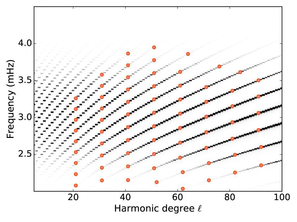
In Fig. 3, we compare the numerical spectrum computed from our analysis with that obtained from $72$ days MDI mode-parameter measurements by Schou [30]. We notice small mismatch between simulated and measured frequencies in Fig. 3. This may be attributed to inaccuracies in our choice of surface boundary conditions as compared to the Sun [27] and the imperfect modeling of surface layers in model S [28].

We assume that the wave propagates through a background that has a sound speed given by

where $\delta c\left(\mathbf{r}\right)$ is a small three-dimensional perturbation to the spherically symmetric sound speed $c_{0}\left(r\right)$ in Model S. The corresponding change $\delta\mathcal{L}$ in the wave operator $\mathcal{L}$ takes the form

where $\mathbf{G}_{r}=(G_{rr},G_{\theta r},G_{\phi r})$. Substituting Equation (30) in Equation (28), we obtain the expression for the sound-speed kernel

We have used the reciprocity relation derived from the adjoint nature of the operator [19]

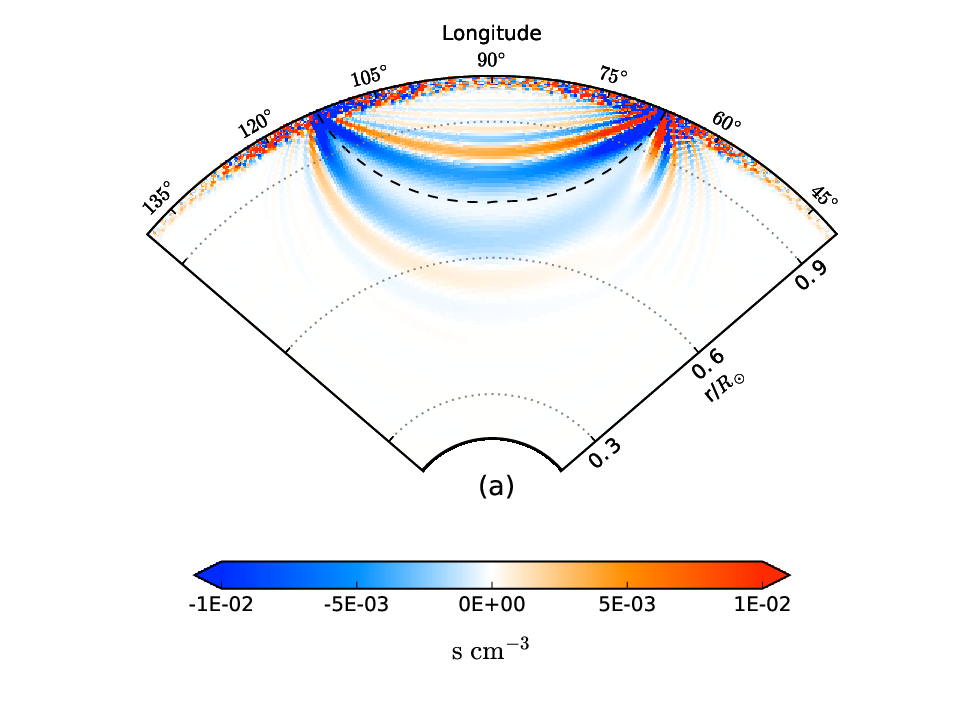
to arrive at the Equation (31). The expression for kernel $K_{c}$ is symmetric on the interchange of the source and receiver location, $\mathbf{r}_{s}$ and $\mathbf{r}_{r}$ and this symmetry can be seen in Fig. 4. The value of the kernel is small near the ray path — as seen in “banana-doughnut” kernels in geophysics literature [23] — and peaks near the source and receiver locations. Fresnel zones surrounding the ray path oscillate between positive and negative values.

In order to validate the sound-speed kernel, we consider the simple scenario where the perturbation in sound speed $\delta c$ is only function of the radius $r$, and the background remains spherically symmetric. In that case, we can solve for Green’s function numerically in a manner similar to that described in Section II, the only change being $c_{0}\rightarrow c_{0}+\delta c$. After obtaining the Green’s function for the perturbed model, we can compute the $\xi_{r}(\mathbf{r}_{r},\mathbf{r}_{s},t)$ from Equation (21). We also obtain the wave displacement $\xi_{r}^{0}(\mathbf{r}_{r},\mathbf{r}_{s},t)$ for Model S through a similar computation. Once we have both $\xi_{r}(\mathbf{r}_{r},\mathbf{r}_{s},t)$ and $\xi_{r}^{0}(\mathbf{r}_{r},\mathbf{r}_{s},t)$, we estimate the change in travel time from Equation (25) and compare it with that obtained from sound-speed kernel (27). In Fig. 5, we plot the results for several different distances between source and receiver for a particular case in which the sound speed of the model is perturbed by $10^{-3}\%$. We find the two estimates of $\delta\tau$ to be in good agreement, demonstrating that the sensitivity kernel has been computed accurately. We also compare the accuracy of the sound-speed kernel by varying the perturbation in sound speed in Fig. (6).

In presence of a temporally stationary flow with a velocity field $\mathbf{v}\left(\mathbf{r}\right)$, there will be an advection term in the wave equation given by

If the velocity field $\mathbf{v}$ is small compared to the sound-speed $c$, the change in travel time $\delta\tau$ is linearly related to $\mathbf{v}$,

where $\mathbf{K}_{\mathbf{v}}$ is the sensitivity kernel for velocity. The expression for $\mathbf{K}_{\mathbf{v}}$ — in the first-order Born approximation — is

where index $j$ is summed over. We compute the $\theta$ and $\phi$ component of the velocity kernel $\mathbf{K}_{\mathbf{v}}$. The basic features of the flow kernel are same as the sound-speed kernel. The expression of kernel $K_{\mathbf{v}}$ is not symmetric in the source and receiver locations, $\mathbf{r}_{s}$ and $\mathbf{r}_{r}$ and this asymmetry is reflected in Fig. (7). The flow kernel also has a small value along the ray path.

Realistic inversions for flows in the Sun should ensure mass conservation. In temporally stationary backgrounds the condition for mass conservation can be expressed as $\bm{\nabla}\cdot\text{$\left(\rho\mathbf{v}\right)$}=0$. The constraint can be enforced automatically if we derive the velocity field from a stream function $\bm{\chi}$. As we are interested in meridional circulation, we follow the approach of Rajaguru & Antia [24] and consider an azimuthal stream function $\bm{\chi}=\chi\left(r,\theta\right)\hat{\bm{\phi}}$. The corresponding velocity field is

We assume that $\chi=0$ at the solar surface. Substituting Equation (36) in Equation (34), we obtain

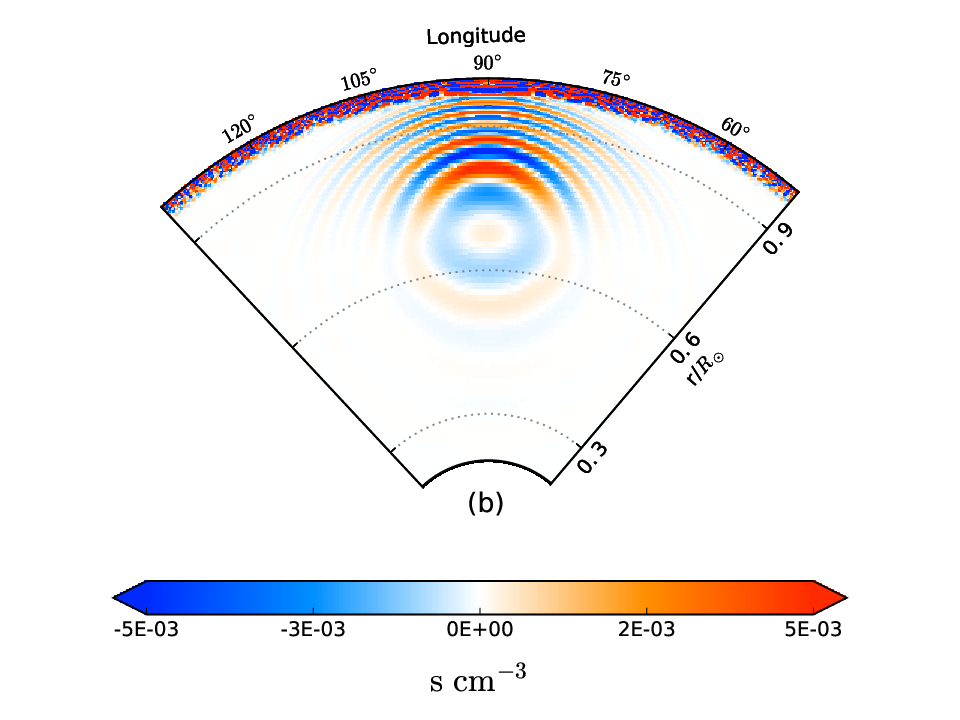
where $K_{\chi}=\hat{\bm{\phi}}\cdot\bm{\nabla}\times\left(\frac{1}{\rho}\mathbf{K}_{\mathbf{v}}\right)$ is the sensitivity kernel for the stream function. We have computed $K_{\chi}$ and it is shown is Fig. (8). The values of this kernel increases rapidly close to the surface, therefore we multiply it with density before plotting to highlight the functional variation with depth. The kernel, $K_{\chi}$ is shown in Fig (8). The grainy pattern near the surface is reminiscent of those observed by Böning et al. [6] and Gizon et al. [17]. It appears due to the finite cutoff in $\ell_{\text{max}}$ chosen to compute the Green’s function. Increasing $\ell_{\text{max}}$ appears to further localize the pattern to shallower layers.

To test the accuracy of the kernel, we consider a flow field equivalent to a solid-body rotation, thereby retaining spherical symmetry. In this case the velocity field will have the form

where $\Omega$ is the angular velocity of the rotation. The perturbed wave field $\bm{\xi}$ will be related to unperturbed wave field $\bm{\xi}_{0}$ through a change in reference frame

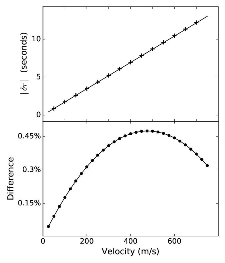
where $\Delta$ is the angular distance between source and receiver. We place both the source and receiver on the equator. Using Equation (39), we compute $\delta\tau$ from Equation (25) and compare it with that obtained from Equation (34). We plot the dependence $\delta\tau$ on the strength of flow velocity in Fig. 9. In Fig. 10, we show the dependence of $\delta\tau$ with source-receiver distance when the flow speed is $20\,\text{m/s}$ at the surface, and compare the difference between the values computed through the two techniques mentioned above.

References

- [1] Bhattacharya, J., Hanasoge, S., & Antia, H. M. 2015, ApJ, 806, 246
- [2] Birch, A. C., & Felder, G. 2004, ApJ, 616, 1261
- [3] Birch, A. C., & Gizon, L. 2007, Astronomische Nachrichten, 328, 228
- [4] Birch, A. C., & Kosovichev, A. G. 2000, Sol. Phys., 192, 193
- [5] Birch, A. C., Kosovichev, A. G., Price, G. H., & Schlottmann, R. B. 2001, ApJ, 561, L229
- [6] Böning, V. G. A., Roth, M., Zima, W., Birch, A. C., & Gizon, L. 2016, ApJ, 824, 49
- [7] Burston, R., Gizon, L., & Birch, A. C. 2015, Space Sci. Rev., 196, 201
- [8] Christensen-Dalsgaard, J., et al. 1996, Science, 272, 1286
- [9] Domingo, V., Fleck, B., & Poland, A. I. 1995, Sol. Phys., 162, 1
- [10] Duvall, Jr., T. L. 1979, Sol. Phys., 63, 3
- [11] Duvall, Jr., T. L., Jefferies, S. M., Harvey, J. W., & Pomerantz, M. A. 1993, Nature, 362, 430
- [12] Giles, P. M. 2000, PhD thesis, STANFORD UNIVERSITY
- [13] Giles, P. M., Duvall, T. L., Scherrer, P. H., & Bogart, R. S. 1997, Nature, 390, 52
- [14] Gizon, L., & Birch, A. C. 2002, ApJ, 571, 966
- [15] —. 2005, Living Reviews in Solar Physics, 2, 6
- [16] Gizon, L., Birch, A. C., & Spruit, H. C. 2010, ARA&A, 48, 289
- [17] Gizon, L., Barucq, H., Duruflé, M., et al. 2016, ArXiv e-prints, arXiv:1611.01666
- [18] Hanasoge, S., Gizon, L., & Sreenivasan, K. R. 2016, Annual Review of Fluid Mechanics, 48, 191
- [19] Hanasoge, S. M., Birch, A., Gizon, L., & Tromp, J. 2011, ApJ, 738, 100
- [20] Houdek, G., Balmforth, N. J., Christensen-Dalsgaard, J., & Gough, D. O. 1999, A&A, 351, 582
- [21] Jackiewicz, J., Gizon, L., Birch, A. C., & Duvall, Jr., T. L. 2007, ApJ, 671, 1051
- [22] Jackiewicz, J., Serebryanskiy, A., & Kholikov, S. 2015, ApJ, 805, 133
- [23] Marquering, H., Dahlen, F. A., & Nolet, G. 1999, Geophysical Journal International, 137, 805
- [24] Rajaguru, S. P., & Antia, H. M. 2015, ApJ, 813, 114
- [25] Rhodes, E. J., Kosovichev, A. G., Schou, J., Scherrer, P. H., & Reiter, J. 1997, Measurements of Frequencies of Solar Oscillations from the MDI Medium-l Program (Dordrecht: Springer Netherlands), 287–310
- [26] Rhodes, Jr., E. J., Reiter, J., Kosovichev, A. G., Schou, J., & Scherrer, P. H. 1998, in ESA Special Publication, Vol. 418, Structure and Dynamics of the Interior of the Sun and Sun-like Stars, ed. S. Korzennik, 73
- [27] Rhodes, Jr., E. J., Reiter, J., Schou, J., Kosovichev, A. G., & Scherrer, P. H. 2001, ApJ, 561, 1127
- [28] Rosenthal, C. S., Christensen-Dalsgaard, J., Nordlund, Å., Stein, R. F., & Trampedach, R. 1999, A&A, 351, 689
- [29] Scherrer, P. H., Bogart, R. S., Bush, R. I., et al. 1995, Sol. Phys., 162, 129
- [30] Schou, J. 1999, ApJ, 523, L181
- [31] Snieder, R. 2004, Physical Review E, 69, 046610
- [32] —. 2007, The Journal of the Acoustical Society of America, 121, 2637
- [33] Zhao, J., Bogart, R. S., Kosovichev, A. G., Duvall, Jr., T. L., & Hartlep, T. 2013, ApJ, 774, L29