A new contribution to discontinuity at fixed point

NİHAL Taş¹ and NİHAL YILMAZ Özgür¹ Address: ¹Balıkesir University, Department of Mathematics, 10145 Balıkesir, TURKEY. Email address: nihaltas@balikesir.edu.tr; nihal@balikesir.edu.tr

Abstract.

The aim of this paper is to obtain new solutions to the open question on the existence of a contractive condition which is strong enough to generate a fixed point but which does not force the map to be continuous at the fixed point. To do this, we use the right-hand side of the classical Rhoades’ inequality and the number $M(x,y)$ given in the definition of an $(\alpha,\beta)$ -Geraghty type- $I$ rational contractive mapping. Also we give an application of these new results to discontinuous activation functions.

Key words and phrases:

Discontinuity, fixed point, fixed circle, metric space, activation function.

2010 Mathematics Subject Classification

Primary 47H10; Secondary 54H25, 47H09.

1. Introduction and Preliminaries

Recently, some solutions to the open question on the existence of contractive conditions which are strong enough to generate a fixed point but which do not force the mapping to be continuous at the fixed point has been proposed and investigated (see [1], [2], [9], [15] and [17] for more details). For example, in [15], Pant proved the following theorem as a solution of this problem.

Theorem 1.1.

[15] If a self-mapping $T$ of a complete metric space $(X,d)$ satisfies the conditions;

(1)

$d(Tx,Ty)\leq\phi\left(\max\left\{d(x,Tx),d(y,Ty)\right\}\right)$ , where $\phi:\mathbb{R}^{+}\rightarrow\mathbb{R}^{+}$ is such that $\phi(t)<t$ for each $t>0,$
(2)

For a given $\varepsilon>0$ , there exists a $\delta(\varepsilon)>0$ such that

$\varepsilon<\max\left\{d(x,Tx),d(y,Ty)\right\}<\varepsilon+\delta\text{,}$

implies $d(Tx,Ty)\leq\varepsilon$ ,

then $T$ has a unique fixed point $z$ . Moreover, $T$ is continuous at $z$ if and only if

\underset{x\rightarrow z}{\lim}\max\left\{d(x,Tx),d(z,Tz)\right\}=0\text{.}

After then, in [1], Bisht and Pant obtained a new solution of the open problem using the number

M(x,y)=\max\left\{d(x,y),d(x,Tx),d(y,Ty),\frac{d(x,Ty)+d(y,Tx)}{2}\right\}\text{.}

Also, in [2], they proved a fixed-point theorem for this problem using the number

N(x,y)=\max\left\{d(x,y),d(x,Tx),d(y,Ty),\frac{\alpha\left[d(x,Ty)+d(y,Tx)\right]}{2}\right\}\text{,}

where $0\leq\alpha<1$ .

Motivated by the above studies, we investigate new contractive conditions to obtain one more solution to the open question. Before stating our main results, we recall the following definitions which are necessary in the next section.

Definition 1.2.

[16] Let $(X,d)$ be a complete metric space and $T$ be a self-mapping of $X$ . $T$ is called a Rhoades’ mapping if the following condition is satisfied for each $x,y\in X$ , $x\neq y:$

d(Tx,Ty)<\max\{d(x,y),d(x,Tx),d(y,Ty),d(x,Ty),d(y,Tx)\}.

Let $\Theta$ be a family of functions $\theta:\left[0,\infty\right)\rightarrow\left[0,1\right)$ such that for any bounded sequence $\left\{t_{n}\right\}$ of positive real numbers, $\theta\left(t_{n}\right)\rightarrow 1$ implies $t_{n}\rightarrow 0$ and $\Phi$ be a family of functions $\phi:\left[0,\infty\right)\rightarrow\left[0,\infty\right)$ such that $\phi$ is continuous, strictly increasing and $\phi(0)=0$ .

Definition 1.3.

[3] Let $(X,d)$ be a metric space, $T:X\rightarrow X$ be a mapping and $\alpha,\beta:X\times X\rightarrow\mathbb{R}^{+}$ . A mapping $T$ is said to be $(\alpha,\beta)$ -Geraghty type- $I$ rational contractive mapping if there exists a $\theta\in\Theta$ , such that for all $x,y\in X$ , the following condition holds $:$

\alpha(x,Tx)\beta(y,Ty)\phi(d(Tx,Ty))\leq\theta(\phi(M(x,y)))\phi(M(x,y))\text{,}

where

M(x,y)=\max\left\{d(x,y),d(x,Tx),d(y,Ty),\frac{d(x,Tx)d(y,Ty)}{1+d(x,y)},\frac{d(x,Tx)d(y,Ty)}{1+d(Tx,Ty)}\right\}

and $\phi\in\Phi$ .

On the other hand, there are some examples of self-mappings which have at least two fixed points. In this case, new fixed-point results are necessary for the existence of fixed points of self-mappings. Also it is important to study the mappings with a fixed circle since there are some applications of these kind mappings to neural networks (see [11] for more details). More recently, some fixed-circle theorems have been presented as a different direction for the generalizations of the known fixed-point theorems (see [12], [13] and [14] for more details).

Now we recall the following definition of a fixed circle and one of the known existence theorems for fixed circles.

Definition 1.4.

[12] Let $(X,d)$ be a metric space and $C_{x_{0},r}=\{x\in X:d(x_{0},x)=r\}$ be a circle. For a self-mapping $T:X\rightarrow X$ , if $Tx=x$ for every $x\in C_{x_{0},r}$ then we call the circle $C_{x_{0},r}$ as the fixed circle of $T$ .

Theorem 1.5.

[12] Let $(X,d)$ be a metric space and $C_{x_{0},r}$ be any circle on $X$ . Let us define the mapping

\varphi:X\rightarrow\left[0,\infty\right)\text{, }\varphi(x)=d(x,x_{0})\text{,}

for all $x\in X$ . If there exists a self-mapping $T:X\rightarrow X$ satisfying

$(C1)$ $d(x,Tx)\leq\varphi(x)-\varphi(Tx)$
and

$(C2)$ $d(Tx,x_{0})\geq r$ ,
for each $x\in C_{x_{0},r}$ , then the circle $C_{x_{0},r}$ is a fixed circle of $T$ .

Our aim in this paper is to obtain new solutions to the open question on the existence of contractive conditions which are strong enough to generate a fixed point but which do not force the mapping to be continuous at the point. In Section 2, we use the right-hand side of the classical Rhoades’ inequality and the number $M(x,y)$ given in the definition of an $(\alpha,\beta)$ -Geraghty type- $I$ rational contractive mapping for this purpose. In Section 3, we give an application of these new results to discontinuous activation functions.

2. Main Results

In this section, we investigate some contractive conditions for the open question mentioned in the introduction.

Theorem 2.1.

Let $(X,d)$ be a complete metric space and $T$ be a self-mapping on $X$ satisfying the following conditions $:$

(1)

There exists a function $\psi:\mathbb{R}^{+}\rightarrow\mathbb{R}^{+}$ such that $\psi(t)<t$ for each $t>0$ and $d(Tx,Ty)\leq\psi(M_{1}(x,y))$ where

M_{1}(x,y)=\max\left\{d(x,y),d(x,Tx),d(y,Ty),\frac{d(x,Tx)d(y,Ty)}{1+d(x,y)},\frac{d(x,Tx)d(y,Ty)}{1+d(Tx,Ty)}\right\};

(2)

There exists a $\delta(\varepsilon)>0$ such that $\varepsilon<M_{1}(x,y)<\varepsilon+\delta$ implies $d(Tx,Ty)\leq\varepsilon$ for a given $\varepsilon>0$ .

Then $T$ has a unique fixed point $y_{0}\in X$ and $T^{n}x\rightarrow y_{0}$ for each $x\in X$ . Also, $T$ is discontinuous at $y_{0}$ if and only if $\underset{x\rightarrow y_{0}}{\lim}M_{1}(x,y_{0})\neq 0$ .

Proof.

Let $x_{0}\in X$ , $x_{0}\neq Tx_{0}$ and the sequence $\left\{x_{n}\right\}$ be defined as $Tx_{n}=x_{n+1}$ for all $n\in\mathbb{N}\cup\left\{0\right\}$ . Using the condition (1), we have

$\displaystyle d(x_{n},x_{n+1})$	$\displaystyle=$	$\displaystyle d(Tx_{n-1},Tx_{n})\leq\psi(M_{1}(x_{n-1},x_{n}))<M_{1}(x_{n-1},x_{n})$
	$\displaystyle=$	$\displaystyle\max\left\{\begin{array}[]{c}d(x_{n-1},x_{n}),d(x_{n-1},x_{n}),d(x_{n},x_{n+1}),\\ \frac{d(x_{n-1},x_{n})d(x_{n},x_{n+1})}{1+d(x_{n-1},x_{n})},\frac{d(x_{n-1},x_{n})d(x_{n},x_{n+1})}{1+d(x_{n},x_{n+1})}\end{array}\right\}$
	$\displaystyle=$	$\displaystyle\max\left\{d(x_{n-1},x_{n}),d(x_{n},x_{n+1})\right\}\text{.}$

Assume that $d(x_{n-1},x_{n})<d(x_{n},x_{n+1})$ . Then from the inequality (2) we get

d(x_{n},x_{n+1})<d(x_{n},x_{n+1})\text{,}

which is a contradiction. So $d(x_{n},x_{n+1})<d(x_{n-1},x_{n})$ and

M_{1}(x_{n-1},x_{n})=\max\left\{d(x_{n-1},x_{n}),d(x_{n},x_{n+1})\right\}=d(x_{n-1},x_{n}).

If we put $d(x_{n},x_{n+1})=u_{n}$ then from the inequality (2) we obtain

u_{n}<u_{n-1}\text{,}

(2.4)

that is, $u_{n}$ is a strictly decreasing sequence of positive real numbers and so the sequence $u_{n}$ tends to a limit $u\geq 0$ .

Suppose that $u>0$ . There exists a positive integer $k\in\mathbb{N}$ such that $n\geq k$ implies

u<u_{n}<u+\delta(u)\text{.}

(2.5)

Using the condition (2) and the inequality (2.4), we get

d(Tx_{n-1},Tx_{n})=d(x_{n},x_{n+1})=u_{n}<u\text{,}

(2.6)

for $n\geq k$ . The inequality (2.6) contradicts to the inequality (2.5). Then it should be $u=0$ .

Now we show that $\left\{u_{n}\right\}$ is a Cauchy sequence. Let us fix an $\varepsilon>0$ . Without loss of generality, we can assume that $\delta(\varepsilon)<\varepsilon$ . There exists $k\in\mathbb{N}$ such that

d(x_{n},x_{n+1})=u_{n}<\delta\text{ }(0<\delta<1)\text{,}

for $n\geq k$ since $u_{n}\rightarrow 0$ . Following Jachymski (see [7] and [8] for more details), using the mathematical induction, we prove

d(x_{k},x_{k+n})<\varepsilon+\delta\text{,}

(2.7)

for any $n\in\mathbb{N}$ . The inequality (2.7) holds for $n=1$ since

d(x_{k},x_{k+1})=u_{k}<\delta<\varepsilon+\delta\text{.}

Assume that the inequality (2.7) is true for some $n$ . We prove it for $n+1$ . Using the triangle inequality, we obtain

d(x_{k},x_{k+n+1})\leq d(x_{k},x_{k+1})+d(x_{k+1},x_{k+n+1})\text{.}

It suffices to show $d(x_{k+1},x_{k+n+1})\leq\varepsilon$ . To do this, we prove $M_{1}(x_{k},x_{k+n})\leq\varepsilon+\delta$ , where

M_{1}(x_{k},x_{k+n})=\max\left\{\begin{array}[]{c}d(x_{k},x_{k+n}),d(x_{k},Tx_{k}),d(x_{k+n},Tx_{k+n}),\\ \frac{d(x_{k},Tx_{k})d(x_{k+n},Tx_{k+n})}{1+d(x_{k},x_{k+n})},\frac{d(x_{k},Tx_{k})d(x_{k+n},Tx_{k+n})}{1+d(Tx_{k},Tx_{k+n})}\end{array}\right\}\text{.}

(2.8)

Using the mathematical induction hypothesis, we find

\begin{array}[]{l}d(x_{k},x_{k+n})<\varepsilon+\delta\text{,}\\ d(x_{k},x_{k+1})<\delta\text{,}\\ d(x_{k+n},x_{k+n+1})<\delta\text{,}\\ \frac{d(x_{k},Tx_{k})d(x_{k+n},Tx_{k+n})}{1+d(x_{k},x_{k+n})}<\frac{\delta^{2}}{1+d(x_{k},x_{k+n})}\text{,}\\ \frac{d(x_{k},Tx_{k})d(x_{k+n},Tx_{k+n})}{1+d(Tx_{k},Tx_{k+n})}<\frac{\delta^{2}}{1+d(Tx_{k},Tx_{k+n})}\text{.}\end{array}

(2.9)

Using the conditions (2.8) and (2.9), we have $M_{1}(x_{k},x_{k+n})<\varepsilon+\delta$ . From the condition (2), we obtain

d(Tx_{k},Tx_{k+n})=d(x_{k+1},x_{k+n+1})\leq\varepsilon\text{.}

Therefore, the inequality (2.7) implies that $\left\{x_{n}\right\}$ is Cauchy. Since $(X,d)$ is a complete metric space, there exists a point $y_{0}\in X$ such that $x_{n}\rightarrow y_{0}$ as $n\rightarrow\infty$ . Also we get $Tx_{n}\rightarrow y_{0}$ .

Now we show that $Ty_{0}=y_{0}$ . On the contrary, suppose that $y_{0}$ is not a fixed point of $T$ , that is, $Ty_{0}\neq y_{0}$ . Then using the condition (1), we get

	$\displaystyle d(Ty_{0},Tx_{n})$	$\displaystyle\leq$	$\displaystyle\psi(M_{1}(y_{0},x_{n}))<M_{1}(y_{0},x_{n})$
		$\displaystyle=$	$\displaystyle\max\left\{\begin{array}[]{c}d(y_{0},x_{n}),d(y_{0},Ty_{0}),d(x_{n},Tx_{n}),\\ \frac{d(y_{0},Ty_{0})d(x_{n},Tx_{n})}{1+d(y_{0},x_{n})},\frac{d(y_{0},Ty_{0})d(x_{n},Tx_{n})}{1+d(Ty_{0},Tx_{n})}\end{array}\right\}$

and so taking limit for $n\rightarrow\infty$ we have

d(Ty_{0},y_{0})<d(y_{0},Ty_{0})=d(Ty_{0},y_{0})\text{,}

which is a contradiction. Thus $y_{0}$ is a fixed point of $T$ . We prove that the fixed point $y_{0}$ is unique. Let $z_{0}$ be another fixed point of $T$ such that $y_{0}\neq z_{0}$ . By the condition (1), we find

$\displaystyle d(Ty_{0},Tz_{0})$	$\displaystyle=$	$\displaystyle d(y_{0},z_{0})\leq\psi(M_{1}(y_{0},z_{0}))<M_{1}(y_{0},z_{0})$
	$\displaystyle=$	$\displaystyle\max\left\{\begin{array}[]{c}d(y_{0},z_{0}),d(y_{0},y_{0}),d(z_{0},z_{0}),\\ \frac{d(y_{0},y_{0})d(z_{0},z_{0})}{1+d(y_{0},z_{0})},\frac{d(y_{0},y_{0})d(z_{0},z_{0})}{1+d(y_{0},z_{0})}\end{array}\right\}$
	$\displaystyle=$	$\displaystyle d(y_{0},z_{0})\text{,}$

which is a contradiction. Hence $y_{0}$ is the unique fixed point of $T$ .

Finally, we prove that $T$ is discontinuous at $y_{0}$ if and only if $\underset{x\rightarrow y_{0}}{\lim}M_{1}(x,y_{0})\neq 0$ . To do this, we show that $T$ is continuous at $y_{0}$ if and only if $\underset{x\rightarrow y_{0}}{\lim}M_{1}(x,y_{0})=0$ . Let $T$ be continuous at the fixed point $y_{0}$ and $x_{n}\rightarrow y_{0}$ . Then $Tx_{n}\rightarrow Ty_{0}=y_{0}$ and

d(x_{n},Tx_{n})\leq d(x_{n},y_{0})+d(Tx_{n},y_{0})\rightarrow 0\text{.}

Hence we get $\underset{n}{\lim}M_{1}(x_{n},y_{0})=0$ . On the other hand, if $\underset{x_{n}\rightarrow y_{0}}{\lim}M_{1}(x_{n},y_{0})=0$ then $d(x_{n},Tx_{n})\rightarrow 0$ as $x_{n}\rightarrow y_{0}$ . This implies $Tx_{n}\rightarrow y_{0}=Ty_{0}$ , that is, $T$ is continuous at $y_{0}$ . ∎

Remark 2.2.

Notice that the conditions $(1)$ and $(2)$ are not independent in Theorem 2.1. Indeed, in the cases where the condition $(2)$ is satisfied, we obtain $d(Tx,Ty)<M_{1}(x,y)$ , where $M_{1}(x,y)>0$ . If $M_{1}(x,y)=0$ then $d(Tx,Ty)=0$ . So the inequality $d(Tx,Ty)\leq\varepsilon$ holds for any $x,y\in X$ with $\varepsilon<M_{1}(x,y)<\varepsilon+\delta$ .

In the following example, we see that a self-mapping satisfying the conditions of Theorem 2.1 has a unique fixed point at which $T$ is discontinuous.

Example 2.3.

Let $X=\left[0,4\right]$ and $d$ be the usual metric on $X$ . Let us define a self-mapping $T:X\rightarrow X$ by

Tx=\left\{\begin{array}[]{ccc}2&;&x\leq 2\\ 0&;&x>2\end{array}\right.\text{.}

Then $T$ satisfies the conditions of Theorem 2.1 and has a unique fixed point $x=2$ at which $T$ is discontinuous. It can be verified in this example that

d(Tx,Ty)=0\text{ and }0<M_{1}(x,y)\leq 4\text{ when }x,y\leq 2\text{,}

d(Tx,Ty)=0\text{ and }2<M_{1}(x,y)\leq 16\text{ when }x,y>2\text{,}

d(Tx,Ty)=2\text{ and }2<M_{1}(x,y)\leq 4\text{ when }x\leq 2\text{, }y>2

and

d(Tx,Ty)=2\text{ and }2<M_{1}(x,y)\leq 4\text{ when }x>2\text{, }y\leq 2\text{.}

Therefore the self-mapping $T$ satisfies the condition $(1)$ given in Theorem 2.1 with

\psi(t)=\left\{\begin{array}[]{ccc}2&;&t>2\\ \frac{t}{2}&;&t\leq 2\end{array}\right.\text{.}

Also $T$ satisfies the condition $(2)$ given in Theorem 2.1 with

\delta(\varepsilon)=\left\{\begin{array}[]{ccc}15&;&\varepsilon\geq 2\\ 5-\varepsilon&;&\varepsilon<2\end{array}\right.\text{.}

It can be easily checked that

\underset{x\rightarrow 2}{\lim}M_{1}(x,2)\neq 0\text{.}

Consequently, $T$ is discontinuous at the fixed point $x=2$ .

Now we give the following corollaries as the results of Theorem 2.1.

Corollary 2.4.

Let $(X,d)$ be a complete metric space and $T$ be a self-mapping on $X$ satisfying the following conditions $:$

(1)

$d(Tx,Ty)\leq M_{1}(x,y)$ for any $x,y\in X$ with $M_{1}(x,y)>0;$
(2)

There exists a $\delta(\varepsilon)>0$ such that $\varepsilon<M_{1}(x,y)<\varepsilon+\delta$ implies $d(Tx,Ty)\leq\varepsilon$ for a given $\varepsilon>0$ .

Corollary 2.5.

Let $(X,d)$ be a complete metric space and $T$ be a self-mapping on $X$ satisfying the following conditions $:$

(1)

There exists a function $\psi:\mathbb{R}^{+}\rightarrow\mathbb{R}^{+}$ such that $\psi(d(x,y))<d(x,y)$ and $d(Tx,Ty)\leq\psi(d(x,y));$
(2)

There exists a $\delta(\varepsilon)>0$ such that $\varepsilon<t<\varepsilon+\delta$ implies $\psi(t)\leq\varepsilon$ for any $t>0$ and a given $\varepsilon>0$ .

Then $T$ has a unique fixed point $y_{0}\in X$ and $T^{n}x\rightarrow y_{0}$ for each $x\in X$ .

In the following theorem, we see that the power contraction of the type $M_{1}(x,y)$ allows the possibility of discontinuity at the fixed point.

Theorem 2.6.

Let $(X,d)$ be a complete metric space and $T$ be a self-mapping on $X$ satisfying the following conditions $:$

(1)

There exists a function $\psi:\mathbb{R}^{+}\rightarrow\mathbb{R}^{+}$ such that $\psi(t)<t$ for each $t>0$ and $d(T^{m}x,T^{m}y)\leq\psi(M_{1}^{\ast}(x,y))$ where

M_{1}^{\ast}(x,y)=\max\left\{\begin{array}[]{c}d(x,y),d(x,T^{m}x),d(y,T^{m}y),\\ \frac{d(x,T^{m}x)d(y,T^{m}y)}{1+d(x,y)},\frac{d(x,T^{m}x)d(y,T^{m}y)}{1+d(T^{m}x,T^{m}y)}\end{array}\right\};

(2)

There exists a $\delta(\varepsilon)>0$ such that $\varepsilon<M_{1}^{\ast}(x,y)<\varepsilon+\delta$ implies $d(T^{m}x,T^{m}y)\leq\varepsilon$ for a given $\varepsilon>0.$

Then $T$ has a unique fixed point. Also, $T$ is discontinuous at $y_{0}$ if and only if $\underset{x\rightarrow y_{0}}{\lim}M_{1}^{\ast}(x,y_{0})\neq 0$ .

Proof.

Using Theorem 2.1, we see that the function $T^{m}$ has a unique fixed point $y_{0}$ , that is, $T^{m}y_{0}=y_{0}$ . Hence we get

Ty_{0}=TT^{m}y_{0}=T^{m}Ty_{0}

and so $Ty_{0}$ is a fixed point of $T^{m}$ . From the uniqueness of the fixed point, then we obtain $Ty_{0}=y_{0}$ . Consequently, $T$ has a unique fixed point. ∎

Remark 2.7.

Using the continuity of the self-mapping $T^{2}$ $($ resp. the continuity of the self-mapping $T^{p}$ , the orbitally continuity of the self-mapping $T)$ and the number $M_{1}(x,y)$ , we can also give new fixed-point results for this open question $($ see [1] and [2] for this approach $)$ .

We give another result of discontinuity at fixed point on a metric space.

Theorem 2.8.

Let $(X,d)$ be a complete metric space and $T$ be a self-mapping on $X$ satisfying the following conditions $:$

(1)

There exists a function $\psi:\mathbb{R}^{+}\rightarrow\mathbb{R}^{+}$ such that $\psi(t)<t$ for each $t>0$ and $d(Tx,Ty)\leq\frac{1}{2}\psi(M_{2}(x,y))$ where

$M_{2}(x,y)=\max\left\{d(x,y),d(Tx,x),d(Ty,y),d(Tx,y),d(Ty,x)\right\};$
(2)

There exists a $\delta(\varepsilon)>0$ such that $\varepsilon<M_{2}(x,y)<\varepsilon+\delta$ implies $d(Tx,Ty)\leq\varepsilon$ for a given $\varepsilon>0$ .

Proof.

Let $x_{0}\in X$ , $x_{0}\neq Tx_{0}$ and a sequence $\left\{x_{n}\right\}$ be defined as $T^{n}x_{0}=Tx_{n}=x_{n+1}$ for all $n\in\mathbb{N}\cup\left\{0\right\}$ . Using the condition (1), we have

$\displaystyle d(x_{n},x_{n+1})$	$\displaystyle=$	$\displaystyle d(Tx_{n-1},Tx_{n})\leq\frac{1}{2}\psi(M_{2}(x_{n-1},x_{n}))<\frac{1}{2}M_{2}(x_{n-1},x_{n})$
	$\displaystyle=$	$\displaystyle\frac{1}{2}\max\left\{\begin{array}[]{c}d(x_{n-1},x_{n}),d(x_{n},x_{n-1}),d(x_{n+1},x_{n}),\\ d(x_{n},x_{n}),d(x_{n+1},x_{n-1})\end{array}\right\}$
	$\displaystyle=$	$\displaystyle\frac{1}{2}\max\left\{d(x_{n-1},x_{n}),d(x_{n+1},x_{n}),d(x_{n+1},x_{n-1})\right\}$
	$\displaystyle<$	$\displaystyle\frac{1}{2}\max\left\{\begin{array}[]{c}d(x_{n-1},x_{n})+d(x_{n+1},x_{n}),d(x_{n+1},x_{n})+d(x_{n-1},x_{n}),\\ d(x_{n+1},x_{n})+d(x_{n},x_{n-1})\end{array}\right\}$
	$\displaystyle=$	$\displaystyle\frac{1}{2}\left[d(x_{n-1},x_{n})+d(x_{n+1},x_{n})\right]$

and so

2d(x_{n},x_{n+1})<d(x_{n-1},x_{n})+d(x_{n+1},x_{n})\text{.}

(2.14)

Using the inequality (2.14), we get

d(x_{n},x_{n+1})<d(x_{n-1},x_{n})\text{.}

If we put $d(x_{n},x_{n+1})=u_{n}$ then from the above inequality we obtain

u_{n}<u_{n-1}\text{,}

(2.15)

that is, $u_{n}$ is a strictly decreasing sequence of positive real numbers and so the sequence $u_{n}$ tends to a limit $u\geq 0$ .

Suppose that $u>0$ . There exists a positive integer $k\in\mathbb{N}$ such that $n\geq k$ implies

u<u_{n}<u+\delta(u)\text{.}

(2.16)

Using the condition (2) and the inequality (2.15), we get

d(Tx_{n-1},Tx_{n})=d(x_{n},x_{n+1})=u_{n}<u\text{,}

(2.17)

for $n\geq k$ . The inequality (2.17) contradicts to the inequality (2.16). Thus it should be $u=0$ .

d(x_{n},x_{n+1})=u_{n}<\frac{\delta}{2}\text{,}

for $n\geq k$ since $u_{n}\rightarrow 0$ . Following Jachymski (see [7] and [8] for more details), using the mathematical induction, we prove

d(x_{k},x_{k+n})<\varepsilon+\frac{\delta}{2}\text{,}

(2.18)

for any $n\in\mathbb{N}$ . The inequality (2.18) holds for $n=1$ since

d(x_{k},x_{k+1})=u_{k}<\frac{\delta}{2}<\varepsilon+\frac{\delta}{2}\text{.}

Assume that the inequality (2.18) is true for some $n$ . We prove it for $n+1$ . Using the triangle inequality, we have

d(x_{k},x_{k+n+1})\leq d(x_{k},x_{k+1})+d(x_{k+1},x_{k+n+1})\text{.}

It suffices to show $d(x_{k+1},x_{k+n+1})\leq\varepsilon$ . To do this, we prove $M_{2}(x_{k},x_{k+n})\leq\varepsilon+\delta$ , where

$\displaystyle M_{2}(x_{k},x_{k+n})$	$\displaystyle=$	$\displaystyle\max\left\{\begin{array}[]{c}d(x_{k},x_{k+n}),d(Tx_{k},x_{k}),d(Tx_{k+n},x_{k+n}),\\ d(Tx_{k},x_{k+n}),d(Tx_{k+n},x_{k})\end{array}\right\}$
	$\displaystyle=$	$\displaystyle\max\left\{\begin{array}[]{c}d(x_{k},x_{k+n}),d(x_{k+1},x_{k}),d(x_{k+n+1},x_{k+n}),\\ d(x_{k+1},x_{k+n}),d(x_{k+n+1},x_{k})\end{array}\right\}$
	$\displaystyle\leq$	$\displaystyle\max\left\{\begin{array}[]{c}d(x_{k},x_{k+n}),d(x_{k},x_{k+1}),d(x_{k+n},x_{k+n+1}),\\ d(x_{k},x_{k+1})+d(x_{k},x_{k+n}),d(x_{k+n},x_{k+n+1})+d(x_{k},x_{k+n})\end{array}\right\}\text{.}$

Using the mathematical induction hypothesis, we get

\begin{array}[]{l}d(x_{k},x_{k+n})<\varepsilon+\frac{\delta}{2}\text{,}\\ d(x_{k},x_{k+1})<\frac{\delta}{2}\text{,}\\ d(x_{k+n},x_{k+n+1})<\frac{\delta}{2}\text{,}\\ d(x_{k},x_{k+1})+d(x_{k},x_{k+n})<\varepsilon+\delta\text{,}\\ \frac{d(x_{k+n},x_{k+n+1})+d(x_{k},x_{k+n})}{2}<\varepsilon+\delta\text{.}\end{array}

(2.28)

Using the conditions (2) and (2.28), we have $M_{2}(x_{k},x_{k+n})<\varepsilon+\delta$ . From the condition (2), we obtain

d(Tx_{k},Tx_{k+n})=d(x_{k+1},x_{k+n+1})\leq\varepsilon\text{.}

Therefore, the inequality (2.18) implies that $\left\{x_{n}\right\}$ is Cauchy. Since $(X,d)$ is a complete metric space, there exists a point $y_{0}\in X$ such that $x_{n}\rightarrow y_{0}$ as $n\rightarrow\infty$ . Also we get $Tx_{n}\rightarrow y_{0}$ .

Now we show that $Ty_{0}=y_{0}$ . On the contrary, $y_{0}$ is not a fixed point of $T$ , that is, $Ty_{0}\neq y_{0}$ . Then using the condition (1), we get

	$\displaystyle d(Ty_{0},Tx_{n})$	$\displaystyle\leq$	$\displaystyle\frac{1}{2}\psi(M_{2}(y_{0},x_{n}))<\frac{1}{2}M_{2}(y_{0},x_{n})$
		$\displaystyle=$	$\displaystyle\frac{1}{2}\max\left\{\begin{array}[]{c}d(y_{0},x_{n}),d(Ty_{0},y_{0}),d(Tx_{n},x_{n}),\\ d(Ty_{0},x_{n}),d(Tx_{n},y_{0})\end{array}\right\}$

and so taking limit for $n\rightarrow\infty$ we have

d(Ty_{0},y_{0})<\frac{1}{2}d(Ty_{0},y_{0})\text{,}

$\displaystyle d(Ty_{0},Tz_{0})$	$\displaystyle=$	$\displaystyle d(y_{0},z_{0})\leq\frac{1}{2}\psi(M_{2}(y_{0},z_{0}))<\frac{1}{2}M_{2}(y_{0},z_{0})$
	$\displaystyle=$	$\displaystyle\frac{1}{2}\max\left\{\begin{array}[]{c}d(y_{0},z_{0}),d(y_{0},y_{0}),d(z_{0},z_{0}),\\ d(y_{0},z_{0}),d(z_{0},y_{0})\end{array}\right\}$
	$\displaystyle=$	$\displaystyle\frac{1}{2}d(y_{0},z_{0})\text{,}$

which is a contradiction. Hence $y_{0}$ is a unique fixed point of $T$ .

Finally, we prove that $T$ is discontinuous at $y_{0}$ if and only if $\underset{x\rightarrow y_{0}}{\lim}M_{2}(x,y_{0})\neq 0$ . To do this, we show that $T$ is continuous at $y_{0}$ if and only if $\underset{x\rightarrow y_{0}}{\lim}M_{2}(x,y_{0})=0$ . Let $T$ be continuous at the fixed point $y_{0}$ and $x_{n}\rightarrow y_{0}$ . Then $Tx_{n}\rightarrow Ty_{0}=y_{0}$ and

d(x_{n},Tx_{n})\leq d(x_{n},y_{0})+d(Tx_{n},y_{0})\rightarrow 0\text{.}

Hence we get $\underset{n}{\lim}M_{2}(x_{n},y_{0})=0$ . On the other hand, if $\underset{x_{n}\rightarrow y_{0}}{\lim}M_{2}(x_{n},y_{0})=0$ then $d(x_{n},Tx_{n})\rightarrow 0$ as $x_{n}\rightarrow y_{0}$ . This implies $Tx_{n}\rightarrow y_{0}=Ty_{0}$ , that is, $T$ is continuous at $y_{0}$ . ∎

In the following example, we see that the self-mapping satisfying the conditions of Theorem 2.8 has a unique fixed point at which $T$ is continuous.

Example 2.9.

Let $X=\left[0,4\right]$ and $d$ be the usual metric on $X$ . Let us define a self-mapping $T:X\rightarrow X$ by

Tx=2\text{,}

for all $x\in X$ . Then $T$ satisfies the conditions of Theorem 2.8 and has a unique fixed point $x=2$ at which $T$ is continuous. It can be verified in this example that

d(Tx,Ty)=0\text{ and }0\leq M_{2}(x,y)\leq 4\text{ when }x,y\in X\text{.}

Therefore the self-mapping $T$ satisfies the condition $(1)$ given in Theorem 2.8 with

\psi(t)=\frac{t}{2}\text{.}

Also $T$ satisfies the condition $(2)$ given in Theorem 2.8 with

\delta(\varepsilon)=5-\varepsilon\text{.}

It can be easily checked that

\underset{x\rightarrow 2}{\lim}M_{2}(x,2)=0\text{.}

Consequently, $T$ is continuous at the fixed point $x=2$ .

Now we give the following corollaries as the results of Theorem 2.8.

Corollary 2.10.

Let $(X,d)$ be a complete metric space and $T$ be a self-mapping on $X$ satisfying the following conditions $:$

(1)

$d(Tx,Ty)\leq\frac{M_{2}(x,y)}{2}$ for any $x,y\in X$ with $M_{2}(x,y)>0;$
(2)

There exists a $\delta(\varepsilon)>0$ such that $\varepsilon<M_{2}(x,y)<\varepsilon+\delta$ implies $d(Tx,Ty)\leq\varepsilon$ for a given $\varepsilon>0$ .

Corollary 2.11.

Let $(X,d)$ be a complete metric space and $T$ be a self-mapping on $X$ satisfying the following conditions $:$

(1)

There exists a function $\psi:\mathbb{R}^{+}\rightarrow\mathbb{R}^{+}$ such that $\psi(d(x,y))<d(x,y)$ and $d(Tx,Ty)\leq\frac{1}{2}\psi(d(x,y))$ ;
(2)

There exists a $\delta(\varepsilon)>0$ such that $\varepsilon<t<\varepsilon+\delta$ implies $\psi(t)\leq\varepsilon$ for any $t>0$ and a given $\varepsilon>0$ .

Then $T$ has a unique fixed point $y_{0}\in X$ and $T^{n}x\rightarrow y_{0}$ for each $x\in X$ .

In the following theorem, we can see that the power contraction of the type $M_{2}(x,y)$ allows the possibility of discontinuity at the fixed point.

Theorem 2.12.

Let $(X,d)$ be a complete metric space and $T$ be a self-mapping on $X$ satisfying the following conditions $:$

(1)

There exists a function $\psi:\mathbb{R}^{+}\rightarrow\mathbb{R}^{+}$ such that $\psi(t)<t$ for each $t>0$ and $d(T^{m}x,T^{m}y)\leq\frac{1}{2}\psi(M_{2}^{\ast}(x,y))$ where

$M_{2}^{\ast}(x,y)=\max\left\{d(x,y),d(T^{m}x,x),d(T^{m}y,y),d(T^{m}x,y),d(T^{m}y,x)\right\};$
(2)

There exists a $\delta(\varepsilon)>0$ such that $\varepsilon<M_{2}^{\ast}(x,y)<\varepsilon+\delta$ implies $d(T^{m}x,T^{m}y)\leq\varepsilon$ for a given $\varepsilon>0.$

Then $T$ has a unique fixed point. Also, $T$ is discontinuous at $y_{0}$ if and only if $\underset{x\rightarrow y_{0}}{\lim}M_{2}^{\ast}(x,y_{0})\neq 0$ .

Proof.

Using Theorem 2.8, we see that the function $T^{m}$ has a unique fixed point $y_{0}$ , that is, $T^{m}y_{0}=y_{0}$ . Hence we get

Ty_{0}=TT^{m}y_{0}=T^{m}Ty_{0}

and so $Ty_{0}$ is a fixed point of $T^{m}$ . From the uniqueness of the fixed point, then we obtain $Ty_{0}=y_{0}$ . Consequently, $T$ has a unique fixed point. ∎

Remark 2.13.

Using the continuity of the self-mapping $T^{2}$ $($ resp. the continuity of the self-mapping $T^{p}$ , the orbitally continuity of the self-mapping $T)$ and the number $M_{2}(x,y)$ , we can also give new fixed-point results for this open question $($ see [1] and [2] for this approach $)$ .

3. An Application of the Main Results to Discontinuous Activation Functions in Neural Networks

Discontinuous activation functions in neural networks have been become important and frequently do arise in practise (see [6] and [10] for more details). In this section, we give an application of the results obtained in Section 2 to discontinuous activation functions. Recently, this topic has been extensively studied.

In [19], the multistability analysis was investigated for neural networks with a class of continuous (but not monotonically increasing) Mexican-hat-type activation functions defined by

T_{i}x=\left\{\begin{array}[]{ccc}m_{i}&;&-\infty<x<p_{i}\\ l_{i,1}x+c_{i,1}&;&p_{i}\leq x\leq r_{i}\\ l_{i,2}x+c_{i,2}&;&r_{i}<x\leq q_{i}\\ m_{i}&;&q_{i}<x<+\infty\end{array}\right.\text{,}

(3.1)

where $p_{i},$ $r_{i},$ $q_{i},$ $m_{i},$ $l_{i,1},$ $l_{i,2},$ $c_{i,1}$ and $c_{i,2}$ are constants with $-\infty<p_{i}<r_{i}<q_{i}<+\infty$ , $l_{i,1}>0$ and $l_{i,2}<0$ , $i=1,2,\ldots,n$ .

In [10], with the inspiration from the continuous Mexican-hat-type activation function (3.1), a general class of discontinuous activation functions was defined by

T_{i}x=\left\{\begin{array}[]{ccc}u_{i}&;&-\infty<x<p_{i}\\ l_{i,1}x+c_{i,1}&;&p_{i}\leq x\leq r_{i}\\ l_{i,2}x+c_{i,2}&;&r_{i}<x\leq q_{i}\\ v_{i}&;&q_{i}<x<+\infty\end{array}\right.\text{,}

(3.2)

where $p_{i},$ $r_{i},$ $q_{i},$ $u_{i},$ $v_{i},$ $l_{i,1},$ $l_{i,2},$ $c_{i,1}$ and $c_{i,2}$ are constants with $-\infty<p_{i}<r_{i}<q_{i}<+\infty$ , $l_{i,1}>0$ , $l_{i,2}<0$ , $u_{i}=l_{i,1}p_{i}+c_{i,1}=l_{i,2}q_{i}+c_{i,2}$ , $l_{i,1}r_{i}+c_{i,1}=l_{i,2}r_{i}+c_{i,2}$ , $v_{i}>T_{i}r_{i}$ , $i=1,2,\ldots,n$ . It can be easily seen that the function $T_{i}x$ is continuous in $\mathbb{R}$ except the point of discontinuity $x=q_{i}$ . Then, it was studied the problem of multistability of competitive neural networks with discontinuous activation functions (see [10] for more details).

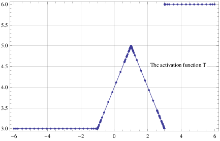
Refer to caption — Figure 1. The graphic of the discontinuous activation function given in (3.3).

To obtain an application of our results given in the previous section, now we take

\begin{array}[]{l}p_{i}=-1,r_{i}=1,q_{i}=3,\\ u_{i}=3,v_{i}=6,l_{i,1}=1,\\ c_{i,1}=4,l_{i,2}=-1,c_{i,2}=6\text{,}\end{array}

in (3.2) to get the following discontinuous activation function:

Tx=\left\{\begin{array}[]{ccc}3&;&-\infty<x<-1\\ x+4&;&-1\leq x\leq 1\\ -x+6&;&1<x\leq 3\\ 6&;&3<x<+\infty\end{array}\right.\text{.}

(3.3)

The function $Tx$ has two fixed points $x_{1}=3$ and $x_{2}=6$ . Since we have $\underset{x\rightarrow 6}{\lim}M_{1}(x,6)=0$ $\left(\text{resp. }\underset{x\rightarrow 6}{\lim}M_{2}(x,6)=0\right)$ , $T$ is continuous at the fixed point $6$ . But, there is not a limit of $M_{1}(x,3)$ $\left(\text{resp. }M_{2}(x,3)\right)$ as $x\rightarrow 3$ and so $T$ is discontinuous at the fixed point $3$ $($ see Figure 1 $)$ . Consequently, using the numbers $M_{1}(x,y)$ and $M_{2}(x,y)$ we can see that the activation function defined in (3.3) is discontinuous at which fixed points.

More generally, in the case that the number of the fixed points of an activation function is greater than two, our results will become important to determine the discontinuity at fixed points. We note that fixed points can be infinitely many. For example, there are some functions which fix a circle with infinitely many points and these kind functions can be considered as activation functions. For example, in [11] it was used new types of activation functions which fix a circle for a complex valued neural network (CVNN). The existence of fixed points of the complex-valued Hopfield neural network (CVHNN) was guaranteed by using these types of activation functions. By these reasons, now we consider Theorem 1.5 and the number $M_{1}(x,y)$ together. We obtain the following proposition.

Proposition 3.1.

Let $(X,d)$ be a metric space, $T$ be a self-mapping on $X$ and $C_{x_{0},r}$ be a fixed circle of $T$ . Then $T$ is discontinuous at any $x\in C_{x_{0},r}$ if and only if $\underset{z\rightarrow x}{\lim}M_{1}(z,x)\neq 0$ .

Proof.

Let $T$ be a continuous self-mapping at $x\in C_{x_{0},r}$ and $x_{n}\rightarrow x$ . Then $Tx_{n}\rightarrow Tx=x$ and $d(x_{n},Tx_{n})\rightarrow 0$ . Hence we get $\underset{n}{\lim}M_{1}(x_{n},x)=0$ .

On the other hand, if $\underset{x_{n}\rightarrow x}{\lim}M_{1}(x_{n},x)=0$ then $d(x_{n},Tx_{n})\rightarrow 0$ as $x_{n}\rightarrow x$ . This implies $Tx_{n}\rightarrow x=Tx$ , that is, $T$ is continuous at $x$ . ∎

Example 3.2.

If we consider the function $T$ defined in $($ 3.3 $)$ then it is easy to check that $T$ satisfies the conditions of Theorem 1.5 for the circle $C_{x_{0},r}=\left\{3,6\right\}$ with the center $x_{0}=\frac{9}{2}$ and the radius $r=\frac{3}{2}$ . Therefore $T$ fixes the circle $C_{x_{0},r}=\left\{3,6\right\}$ as another point of view. By the above proposition, it can be easily deduced that the function $T$ is continuous at the point $x_{1}=6$ but is not continuous at $x_{2}=3$ .

Finally, we note that it is possible to use the number $M_{2}(x,y)$ for the investigation of discontinuity at any point on the fixed circle of the activation function.

4. Conclusion

We mention that our main results are applicable to neural nets under suitable conditions (see [4], [5] and [18] for more details). For example, McCulloch-Pitts model is frequently used in Biology and Artificial Intelligence according to the discontinuity at fixed point. Also our main results can be applied on complex-valued metric spaces since discontinuity of functions have been used in various applicable areas such as complex-valued Hopfield neural networks (see [20] for more details).

Acknowledgement. The authors gratefully thank to the Referees for the constructive comments and recommendations which definitely help to improve the readability and quality of the paper.

References

[1] R. K. Bisht and R. P. Pant, A remark on discontinuity at fixed point, J. Math. Anal. Appl. 445 (2017) 1239-1242.
[2] R. K. Bisht and R. P. Pant, Contractive definitions and discontinuity at fixed point, Appl. Gen. Topol. 18 (1) (2017) 173-182.
[3] S. Chandok, Some fixed point theorems for $(\alpha,\beta)$ -admissible Geraghty type contractive mappings and related results, Math. Sci. 9 (2015) 127-135. doi: 10.1007/s40096-015-0159-4
[4] L. J. Cromme and I. Diener, Fixed point theorems for discontinuous mapping, Math. Program. 51 (1991) 257-267.
[5] L. J. Cromme, Fixed point theorems for discontinuous functions and applications, Nonlinear Analysis: Theory, Methods & Applications 30 (3) (1997) 1527-1534.
[6] M. Forti and P. Nistri, Global convergence of neural networks with discontinuous neuron activations, IEEE Trans. Circuits Syst. I, Fundam. Theory Appl. 50 (11) (2003) 1421-1435.
[7] J. Jachymski, Common fixed point theorems for some families of maps, Indian J. Pure Appl. Math. 25 (9) (1994) 925-937.
[8] J. Jachymski, Equivalent conditions and Meir-Keeler type theorems, J. Math. Anal. Appl. 194 (1995) 293-303.
[9] R. Kannan, Some results on fixed points–II, Amer. Math. Monthly 76 (1969) 405-408.
[10] X. Nie and W. X. Zheng, On multistability of competitive neural networks with discontinuous activation functions, Control Conference (AUCC), 2014 4th Australian 245-250.
[11] N. Özdemir, B. B. İskender and N. Y. Özgür, Complex valued neural network with Möbius activation function, Commun. Nonlinear Sci. Numer. Simul. 16 (12) (2011) 4698-4703.
[12] N. Y. Özgür and N. Taş, Some fixed-circle theorems on metric spaces, Bull. Malays. Math. Sci. Soc. (2017). https://doi.org/10.1007/s40840-017-0555-z
[13] N. Y. Özgür and N. Taş, Some fixed-circle theorems on $S$ -metric spaces with a geometric viewpoint, arXiv:1704.08838 [math.MG].
[14] N. Y. Özgür, N. Taş and U. Çelik, Some fixed-circle results on $S$ -metric spaces, Bull. Math. Anal. Appl. 9 (2) (2017) 10-23.
[15] R. P. Pant, Discontinuity and fixed points, J. Math. Anal. Appl. 240 (1999) 284-289.
[16] B. E. Rhoades, A comparison of various definitions of contractive mappings, Trans. Amer. Math. Soc. 226 (1977) 257-290.
[17] B. E. Rhoades, Contractive definitions and continuity, Contemp. Math. 72 (1988) 233-245.
[18] M. J. Todd, The computation of fixed points and applications, Springer-Verlag, Berlin, Heidelberg, New York, 1976.
[19] L. L. Wang and T. P. Chen, Multistability of neural networks with Mexican-hat-type activation functions, IEEE Trans. Neural Netw. Learn. Syst. 23 (11) (2012) 1816-1826.
[20] Z. Wang, Z. Guo, L. Huang and X. Liu, Dynamical behavior of complex-valued Hopfield neural networks with discontinuous activation functions, Neural Process Lett (2016). doi:10.1007/s11063-016-9563-5