Dimensional splitting of hyperbolic partial differential equations using the Radon transform

The Radon transform $\hat{\varphi}:S^{n-1}\times\mathbb{R}\to\mathbb{R}$ of the function $\varphi:\mathbb{R}^{n}\to\mathbb{R}$ is defined as

$$\hat{\varphi}(\omega,s)=\mathcal{R}\varphi(\omega,s)=\int_{x\cdot\omega=s}\varphi(x)\,\textrm{d}m(x),$$

(2.1)

in which $\mathrm{d}m$ is the Euclidean measure over the hyperplane. For any fixed pair $(\omega,s)\in S^{n-1}\times\mathbb{R}$, the set $\{x=(x_{1},x_{2},...,x_{n})\in\mathbb{R}^{n}:x\cdot\omega=s\}$ defines a hyperplane, so the transform is simply an integration of the function over this hyperplane. We will denote the space of hyperplanes parametrized above by $\mathbb{P}^{n}$. In effect, $\hat{\varphi}$ decomposes $\varphi$ into planar waves in the direction of $\omega$.

The back-projection is defined as the dual of $\mathcal{R}$ with respect to the obvious inner product over $S^{n-1}\times\mathbb{R}$. For $\psi:S^{n-1}\times\mathbb{R}\to\mathbb{R}$ the back-projection $\check{\psi}$ is

$$\check{\psi}(x)=\mathcal{R}^{\#}\psi(x)=\int_{S^{n-1}}\psi(\omega,\omega\cdot x)\,\textrm{d}S(\omega),$$

(2.2)

where $\textrm{d}S$ is the measure on $S^{n-1}$.

The Radon transform $\mathcal{R}$ is a linear one-to-one map between $\mathcal{S}(\mathbb{R}^{n})$ and $\mathcal{S}_{H}(\mathbb{P}^{n})$ [18] in which $\mathcal{S}(\mathbb{R}^{n})$ denotes the Schwartz class and

$$\mathcal{S}_{H}(\mathbb{P}^{n})=\left.\begin{cases}&\text{for each }k\in\mathbb{Z}^{+},\int_{\mathbb{R}}F(\omega,p)p^{k}\,\mathrm{d}p\text{ is}\\ F\in\mathcal{S}(\mathbb{P}^{n}):&\text{a homogeneous polynomial in }\omega_{1},...,\omega_{n}\\ &\text{of degree }k\end{cases}\right\}.$$

(2.3)

The correspondence can be naturally extended to distributions, and we refer the reader to standard references for further details.

The Radon transform has a remarkable property, that it intertwines a partial derivative with a univariate derivative. The $i$-th partial derivative $\partial/\partial x_{i}$ of $\varphi$ is now transformed to the derivative of $\hat{\varphi}$ with respect to $s$ multiplied by $\omega_{i}$,

$$\left({\frac{\partial}{\partial x_{i}}\varphi(x)}\right)^{\wedge}=\omega_{i}\frac{\partial}{\partial s}\hat{\varphi}(\omega,s).$$

(2.4)

This is the key property that allows us to transform a multi-dimensional hyperbolic problem into a collection of one-dimensional problems. For example, let us apply the Radon transform to the transport equation in $\mathbb{R}^{2}$, in which the scalar state variable $q:\mathbb{R}^{+}\times\mathbb{R}^{2}\to\mathbb{R}$ satisfies,

$$q_{t}+\theta\cdot\nabla q=0\quad\text{ where }\quad\theta\in S^{1}.$$

(2.5)

The transformation produces a family of 1D advection equations

$$\hat{q}_{t}+(\theta\cdot\omega)\hat{q}_{s}=0,$$

(2.6)

whose coefficient varies for each $\omega$. Similarly, consider the acoustic equations for $p,u,v:\mathbb{R}^{+}\times\mathbb{R}^{2}\to\mathbb{R}$, where the state variable $p$ denotes pressure, $u$ the velocity in $x_{1}$-direction, $v$ the velocity in $x_{2}$-direction,

$$\begin{bmatrix}p\\ u\\ v\end{bmatrix}_{t}+\begin{bmatrix}0&K_{0}&0\\ 1/\rho_{0}&0&0\\ 0&0&0\end{bmatrix}\begin{bmatrix}p\\ u\\ v\end{bmatrix}_{x_{1}}+\begin{bmatrix}0&0&K_{0}\\ 0&0&0\\ 1/\rho_{0}&0&0\end{bmatrix}\begin{bmatrix}p\\ u\\ v\end{bmatrix}_{x_{2}}=0.$$

(2.7)

After the transform, we obtain

$$\begin{bmatrix}\hat{p}\\ \hat{u}\\ \hat{v}\end{bmatrix}_{t}+\begin{bmatrix}0&\omega_{1}K_{0}&\omega_{2}K_{0}\\ \omega_{1}/\rho_{0}&0&0\\ \omega_{2}/\rho_{0}&0&0\end{bmatrix}\begin{bmatrix}\hat{p}\\ \hat{u}\\ \hat{v}\end{bmatrix}_{s}=0.$$

(2.8)

This PDE has one spatial dimension in variable $s$. Letting $\mu=\omega_{1}u+\omega_{2}v$ and $\nu=-\omega_{2}u+\omega_{1}v$, (2.7) can be rewritten as three equations for new states $\hat{p},\hat{\mu}$ and $\hat{\nu}$. If one omits the trivial equation $\nu_{t}=0$, the equation (2.7) is reduced to the 1D acoustic equations,

$$\begin{bmatrix}\hat{p}\\ \hat{\mu}\end{bmatrix}_{t}+\begin{bmatrix}0&K_{0}\\ 1/\rho_{0}&0\end{bmatrix}\begin{bmatrix}\hat{p}\\ \hat{\mu}\end{bmatrix}_{s}=0.$$

(2.9)

In this case, the equation depends on $\omega$ through the variable $\mu$. However, the equation itself is invariant over all $\omega$, owing to the fact that the problem (2.7) is isotropic. Moreover, note that this is exactly the same equation obtained in the physical space if you consider the case of a plane wave where the data varies only in the direction $\omega$ so that derivatives in the orthogonal direction vanish.

The Radon transform therefore transforms $n$-dimensional hyperbolic problems such as (2.5) and (2.7) into their $1$-dimensional counterparts (2.6) and (2.9), respectively.

Previous dimensional splitting methods [28, 37, 14, 25] such as Strang splitting do not allow a natural extension of large time-step (LTS) methods [21, 23, 22] to multiple spatial dimensions. In order to take large time-steps for constant coefficient multi-dimensional hyperbolic problems, one can use the Fourier transform, for example. Upon taking the Fourier transform, one is left with a set of ordinary differential equations (ODEs) different from the original problem [38, 7]. On the other hand, using the Radon transform, one obtains a dimensional splitting that reduces the multi-dimensional problem into a family of one-dimensional counterparts of similar (if not identical) form. This allows 1D LTS methods to be applied for each of these problems, and the multi-dimensional solution is obtained by computing the inverse of the Radon transform. Moreover, the Radon transform provides an intuitive geometrical interpretation as a decomposition into planar waves and thus yields other useful applications. These applications will be illustrated in Section 4.

This multi-dimensional extension of the LTS method for the constant coefficient case is very straightfoward. Taking the Radon tranform of the problem as above, one obtains a set of $1$D problems such as (2.6) or (2.9). Then one applies the $1$D LTS solution operator $\mathcal{K}$ to evolve the initial data $\hat{u}_{0}(\omega,s)$ for each $\omega$ up to desired final time $T$. The operator $\mathcal{K}$ may depend on the direction $\omega$, so we denote the dependence as a parameter by writing $\mathcal{K}=\mathcal{K}(T;\omega)$. This yields the Radon transform of the solution at time $T$,

$$\hat{q}(T,\omega,s)=\mathcal{K}(T;\omega)\hat{q}_{0}(\omega,s).$$

(2.10)

Then, to compute the solution $q$ we can apply the inversion formula

$$c_{n}q(T,x)=\left\{\begin{aligned} &\mathcal{R}^{\#}\frac{d^{n-1}}{ds^{n-1}}\,\hat{q}(T,\omega,s)&\text{ if }n\text{ is odd,}\\ &\mathcal{R}^{\#}H_{s}\frac{d^{n-1}}{ds^{n-1}}\,\hat{q}(T,\omega,s)&\text{ if }n\text{ even,}\\ \end{aligned}\right.$$

(2.11)

where the constant $c_{n}=(4\pi)^{(n-1)/2}\Gamma(n/2)/\Gamma(1/2)$ and $H_{s}$ denotes the Hilbert transform. Much is known about the inversion; see standard texts such as [18, 29] for more details.

This splitting can also be related to the Strang splitting, if one views it as a decomposition of the multi-dimensional problem into planar wave propagation. In Strang splitting one constructs the planar waves emanating in varying directions by dividing a single time-step into multiple successive planar wave propagations. The Radon transform decomposes the multi-dimensional directions by explicitly discretizing the sphere $S^{n-1}$.

Let us consider a concrete example, the 2D acoustic equation (2.7). Let us set $K_{0}=\rho_{0}=1$, so that we have the sound speed $c=1$, and impose the initial conditions

	$\displaystyle q_{0}(x)$	$\displaystyle=\begin{bmatrix}p_{0}(x_{1},x_{2})\\ 0\\ 0\\ \end{bmatrix},$		(2.12)
	$\displaystyle p_{0}(x)$	$\displaystyle=\left\{\begin{aligned} \cos(\pi(x_{1}^{2}+x_{2}^{2})/2)&\quad\text{ if }\,x_{1}^{2}+x_{2}^{2}<1,\\ 0&\quad\text{ otherwise. }\\ \end{aligned}\right.$

The initial pressure profile is a cosine hump supported in a disk of radius $1$ centered at the origin, and the initial velocity profile is identically zero. We will also set absorbing boundary conditions in the manner to be described in Section 4.1.

On the transformed side (2.9), the evolution for any fixed direction $\omega\in S^{1}$ is given by the d’Alembert solution (2.13),

$$\hat{q}(t,\omega,s)=\frac{1}{2}\left(r_{1}\hat{p}_{0}(\omega,s-t)+r_{2}\hat{p}_{0}(\omega,s+t)\right)\quad\text{ where }r_{1}=\begin{bmatrix}1\\ \omega_{1}\\ \omega_{2}\end{bmatrix}\text{ and }r_{2}=\begin{bmatrix}1\\ -\omega_{1}\\ -\omega_{2}\end{bmatrix}.$$

(2.13)

This reduces to simple shifts at corresponding speeds, which can be computed easily up to any time $t$. This is precisely the 1D LTS solution for the constant coefficient case.

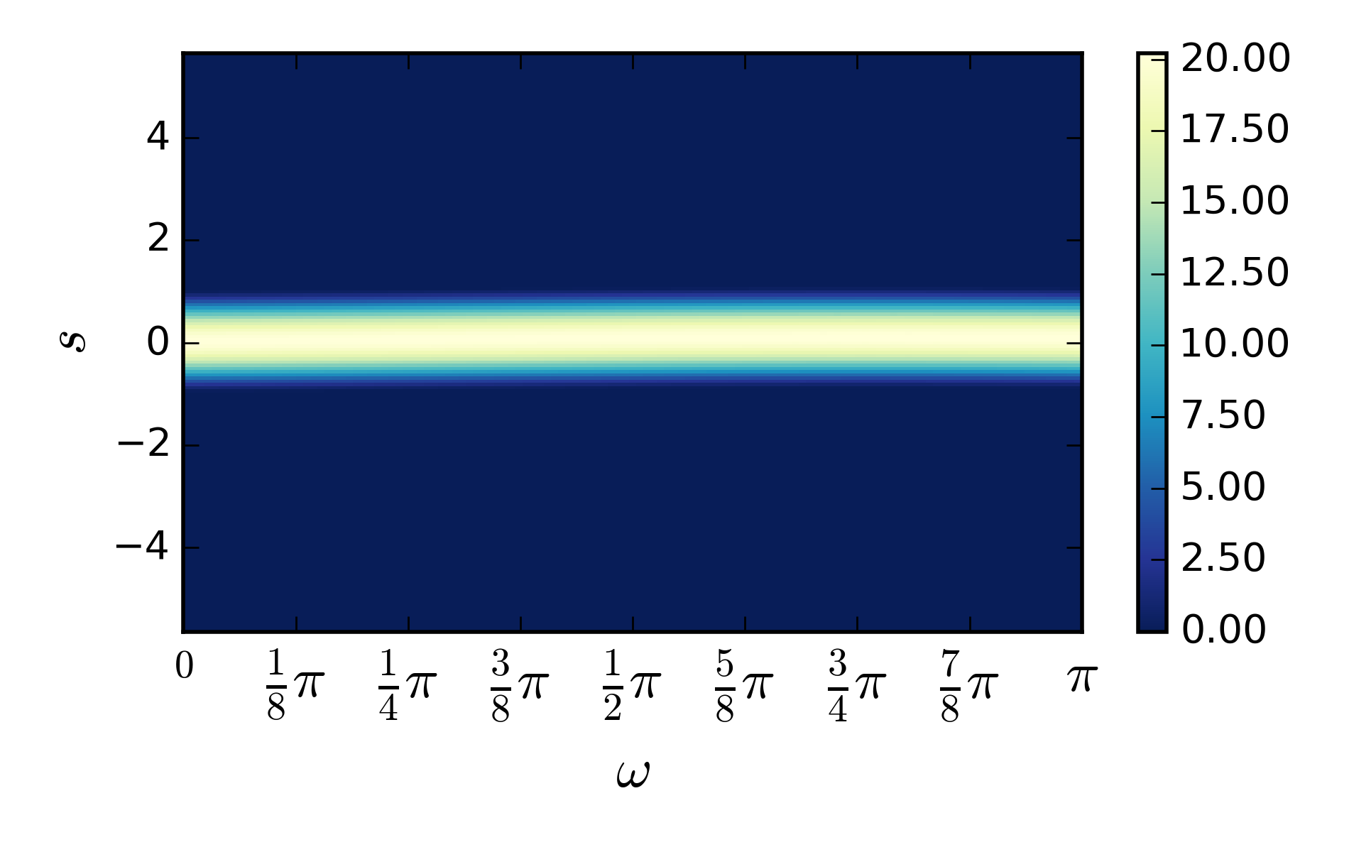
The solution to the acoustic equation computed on the domain $[-4,4]\times[-4,4]$ is shown in the left column of Figure 1. The Radon transform of the pressure term $\hat{p}$ is plotted in the right column of the same figure. Note that this problem is radially symmetric about the origin. A consequence of this is that the Radon transform is invariant with respect to the variable $\omega$, hence the Radon transform of the solutions at different times all appear as horizontal stripes. (There is a small amount of shift, following from the fact that for an image of even size $N$, the origin is chosen as the $(N/2,N/2)$-pixel, slightly off center.)

A key observation is that the evolution of the solution in the transformed variables is a sum of two shifting horizontal stripes, although the wave profile in the spatial domain propagates radially. For each fixed angle $\omega$, one only need solve the d’Alembert solution (2.13), which is easy to solve to any time $t$ by shifting the initial profile twice each according to two opposite speeds, and summing them. Intuitively, the shifts correspond to the propagation of decomposed planar waves for any fixed normal directions in $S^{1}$.

The actual computational did not make use of the continuous Radon transform (2.1), but rather a completely discrete approximation called the DRT, which will be introduced and discussed in further detail in Section 3. Here it will suffice to mention that a grid of size $128\times 128$ was used and prologation of $p=2$ was used for the DRT, and that the continuous transform can be obtained by an easy change of variables (3.5) which scale the domain and amplitude of the DRT, and that the change of variables do not affect the intertwining property. The 1D LTS method can still be used on the DRT, just as in the case of the continuous transform. The computational cost for this solution is conjectured to be $\mathcal{O}(N^{5/2}\log N)$: $\mathcal{O}(N^{2}\log N)$ for the forward DRT, $\mathcal{O}(N^{2})$ for the 1D LTS solution, and $\mathcal{O}(N^{5/2}\log N)$ for the inverse DRT (see Section 3). We note that the 1D LTS method can be applied for each angle in parallel.

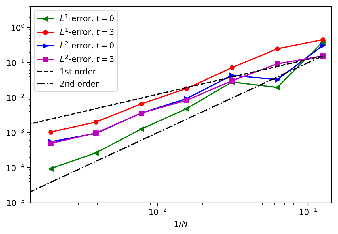
Since the problem is radially symmetric, we can compare the solution to a 1D reference solution of high accuracy. We computed the 1D problem using Godunov flux with 4000 grid cells, as implemented in the Clawpack software package [12]. We compared the diagonal slice of our 2D solution at angle $\pi/4$ with the reference solution at time $t=0$ and $t=3$. To observe the accuracy of the solution with respect to the grid-size, solutions of sizes $N=8,16,32,64,128,256,512$ are also compared. The error was computed for the pressure variable $p$ using the weighted $L^{1}$ and $L^{2}$ norms,

		$\displaystyle\left(\int_{0}^{4\sqrt{2}}|p(\rho,t)-p_{\textrm{ref}}(\rho,t)|^{\mathfrak{p}}\rho\,\textrm{d}\rho\right)^{\frac{1}{\mathfrak{p}}}$		(2.14)
		$\displaystyle\text{ where }\rho=\sqrt{x_{1}^{2}+x_{2}^{2}},\quad p(\rho,t)=p\left(\frac{\rho}{\sqrt{2}},\frac{\rho}{\sqrt{2}},t\right),\quad\mathfrak{p}=1,2.$

The comparison results are displayed in Figure 3. The error at the later time is at the level of the initial discretization error. We also observe that the convergence rate is between first and second-order with respect to the cell diameter $1/N$.

While this particular problem was radially symmetric, the splitting is by no means restricted to problems with radial symmetry. Let us modify the initial conditions above so that it is the sum of two cosine humps of different radii and heights,

	$\displaystyle q_{0}(x)$	$\displaystyle=\begin{bmatrix}p_{1}(x_{1},x_{2})\\ 0\\ 0\\ \end{bmatrix},$		(2.15)
	$\displaystyle p_{1}(x)$	$\displaystyle=p_{0}(x_{1}+1,x_{2}+1.5)+1.5\,p_{0}(1.25(x_{1}-0.75),1.25(x_{2}-1.1)).$

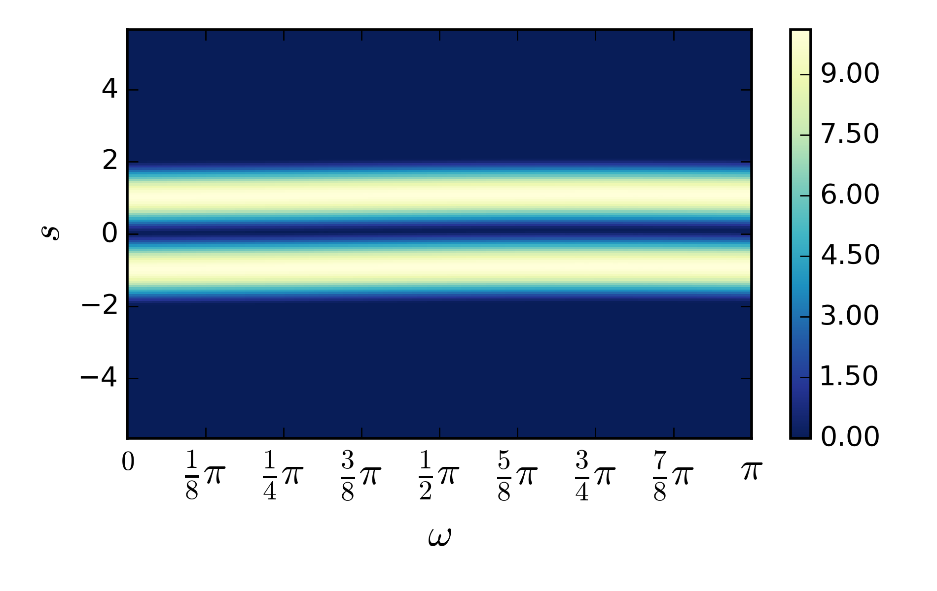
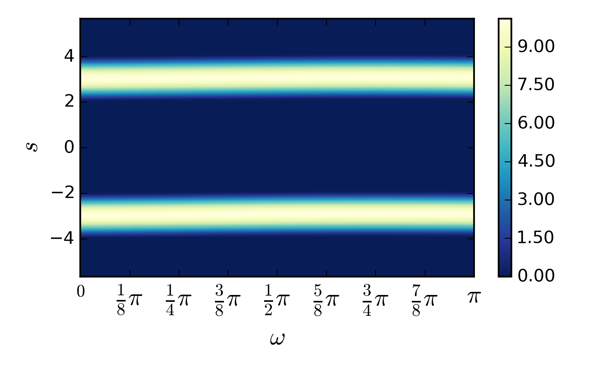
The splitting solution and its continuous Radon transform is plotted in Figure 2. In the first row of the figure, the initial condition and its Radon transform are shown. The two cosine humps in the initial condition each correspond to a sinusoidal signal on the transformed side. Recall the horizontal line centered at $s=0$ from the previous example (Figure 1). The sinusoidal shift away from $s=0$ is due to the fact that translation is an anisotropic operation. This can also be deduced from the transformed transport equation (2.6) in which the transport speed is $\theta\cdot\omega$, that is, $\cos\phi$ where $\phi$ is the angle between transport direction $\theta$ and the direction of the transform $\omega$. For example, when the cosine hump at the origin $p_{0}$ (2.12) is transported away from the origin by $r(\theta\cdot\omega)$, $\hat{p_{0}}$ is shifted by $\hat{p_{0}}(\omega,s-r\cos(\phi))$.

In any case, the solution is still given by the d’Alembert solution (2.13) and the acoustics equation can be solved exactly the same way as before. The DRT used in the actual computations are plotted in Figure 7. Each corresponds to a continuous transform in Figure 2.

Here we will discuss how the splitting above to can be applied to a fully nonlinear system of hyperbolic equations. For a state vector $q$, such a PDE is given in the form

$$q_{t}+f(q)_{x_{1}}+g(q)_{x_{2}}=0,$$

(2.16)

where $f$ and $g$ are flux functions that can be nonlinear. Taking the Radon transform as before, we obtain

$$\hat{q}_{t}+\left[\omega_{1}f(q)+\omega_{2}g(q)\right]^{\wedge}_{s}=0.$$

(2.17)

Let us define the directional flux function as

$$h(q)=\omega_{1}f(q)+\omega_{2}g(q).$$

(2.18)

Then one obtains the nonlinear $1$D equations,

$$\hat{q}_{t}+h(q)^{\wedge}_{s}=0.$$

(2.19)

As in the acoustics equation (2.9), the dependence on $\omega$ enters through the flux function $h(q)$, while the form of the equation is invariant with respect to $\omega$.

As an example, consider the shallow water equations in 2D, in which $\rho,u,v:\mathbb{R}^{+}\times\mathbb{R}^{2}\to\mathbb{R}$ denote water height, velocity in the $x_{1}$-direction and velocity in the $x_{2}$-direction, respectively,

$$\begin{bmatrix}\rho\\ \rho u\\ \rho v\\ \end{bmatrix}_{t}+\begin{bmatrix}\rho u\\ \rho u^{2}+\frac{1}{2}\bar{g}\rho^{2}\\ \rho uv\end{bmatrix}_{x_{1}}+\begin{bmatrix}\rho v\\ \rho uv\\ \rho v^{2}+\frac{1}{2}\bar{g}\rho^{2}\end{bmatrix}_{x_{2}}=0.$$

(2.20)

Here $\bar{g}$ denotes the gravitational constant. The Radon transform as above yields $1$D equation in the form (2.19), in the transformed velocity variables $\mu=\omega_{1}u+\omega_{2}v$ and $\nu=-\omega_{2}u+\omega_{1}v$,

$$\begin{bmatrix}\rho\\ \rho\mu\\ \rho\nu\\ \end{bmatrix}^{\wedge}_{t}+\begin{bmatrix}\rho\mu\\ \rho\mu^{2}+\frac{1}{2}\bar{g}\rho^{2}\\ \rho\mu\nu\end{bmatrix}^{\wedge}_{s}=0.$$

(2.21)

Note that the first two equations of (2.21) are just the shallow water equation in a single dimension in the normal direction of the hyperplane, whereas the third equation is the conservation of momentum in the transverse direction.

We observe that the transformed equations resemble a finite volume discretization. Let us say that $\xi_{i,j}$ is a discretization of the hyperplane $\{x\in\mathbb{R}^{n}:x\cdot\omega_{i}=s_{j}\}$. The specific discretization for the hyperplanes can take on many different forms, but here we will leave it in a general form. We denote the approximation to $\hat{q}(t_{n},\omega_{i},s_{j})$ at time-step $t_{n}$ by $\hat{Q}^{n}_{i,j}$,

$$\hat{Q}_{i,j}^{n}\approx\int_{\xi_{i,j}}q(t_{n},x)\,\textrm{d}m(x).$$

(2.22)

For each fixed direction $i=i_{0}$, the collection of hyperplanes $\{\xi_{i_{0},j}\}$ form a partition of the domain. We can consider these hyperplanes to be finite volume cells. In the equation (2.19) the flux function $h(q)$ assigns the flux between $\xi_{i_{0},j}$ and $\xi_{i_{0},j+1}$. If the cell boundary between $\xi_{i_{0},j}$ and $\xi_{i_{0},j+1}$ is denoted by $\xi_{i_{0},j+\frac{1}{2}}$, we define the numerical flux $F_{i_{0},j+\frac{1}{2}}^{n}$ to be an approximation to the flux at $\xi_{i_{0},j+\frac{1}{2}}$, valid from time-step $t_{n}$ to $t_{n+1}$. Then we have the finite volume update

$$\hat{Q}^{n+1}_{i_{0},j}=\hat{Q}^{n}_{i_{0},j}-\Delta t(F_{i_{0},j+\frac{1}{2}}^{n}-F_{i_{0},j-\frac{1}{2}}^{n}).$$

(2.23)

Once these updates are made for all $i$, the updated $\hat{Q}^{n+1}_{i,j}$ are combined through the inversion formula (2.11) to yield the numerical solution at time $t_{n+1}$.

The dimensional splitting strategy would be to compute the numerical flux $F^{n}_{i,j+\frac{1}{2}}$ by solving only the 1D Riemann problems in the $x$ and $y$ directions. Since the flux function $h(q)$ is a linear combination of normal fluxes $f(q)$ and $g(q)$ (2.18), we can compute $h$ once we have the approximation for these normal fluxes. In other words, we can solve the $1$D Riemann problems for piecewise constant jumps locally in $x$ and $y$ directions, then sum these fluxes across the cell boundary $\xi_{i,j+\frac{1}{2}}$ to obtain the flux between hyperplanes. One thereby decomposes the multi-dimensional Riemann problem into a set of single-dimensional ones, to be combined together by the inversion formula (2.11).

Unlike in the constant coefficient case, the flux function $h(q)$ must be updated at every time step, as is usually done for finite volume methods, although one may apply the nonlinear LTS method on the transformed problem regardless. This would be based on the 1D analogues studied in [21, 23, 22]. The fully nonlinear splitting will not be implemented here, but will be investigated in a future work.

The d-lines of length $N$ are denoted by $D_{N}(h,s)$ with two parameters $h$ and $s$ (see Figure 4.) $h$ denotes the height ($x$-intercept) and $s$ the slope ($x$-displacement), and the pair corresponds to $s$ and $\boldsymbol{\omega}$ for the continuous transform (2.4), respectively. Although the same notation $s$ is used here again after having been used in the continuous setting (2.1) we will keep the notation in order to follow the intuitive notation of [30], and mark the continuous variable with a subscript $s_{c}$ whenever the two are used simultaneously. The definition uses the recursion in which d-lines of length $2n$ are split into left and right d-lines of half its length,

	$\displaystyle D_{2n}(h,2s)$	$\displaystyle=D^{L}_{n}(h,s)\cup D^{R}_{n}(h+s,s),$		(3.1)
	$\displaystyle D_{2n}(h,2s+1)$	$\displaystyle=D^{L}_{n}(h,s)\cup D^{R}_{n}(h+s+1,s).$

The recursion (3.1) defines only a quarter of the possible d-lines, as the slope $s$ will range from 0 to $N$, corresponding to angles $0$ to $\pi/4$ starting from the $x$-axis in the counter-clockwise direction. This is referred to by saying that the d-lines cover one quadrant, for the full transform one needs to cover the angles from $0$ to $\pi$. The other d-lines can be computed by transposing and flipping the indices $h$ and $s$. We will denote the d-lines and DRT corresponding to the angular intervals $[0,\pi/4]$,$[\pi/4,\pi/2]$,$[\pi/2,3\pi/4]$, and $[3\pi/4,\pi]$ by $a$,$b$,$c$, and $d$.

The DRT of an array $A\in\mathbb{R}^{2}$ for the quadrants $a,b,c$ and $d$ are given by the summation of entries of $A$ over the d-lines,

	$\displaystyle\left(\mathcal{R}_{N}^{a}A\right)_{h,s}$	$\displaystyle=\sum_{(i,j)\in D_{N}(h,s)}A_{i,j},$		(3.2)
	$\displaystyle\left(\mathcal{R}_{N}^{b}A\right)_{h,s}$	$\displaystyle=\sum_{(i,j)\in D_{N}(h,s)}A_{j,i},$
	$\displaystyle\left(\mathcal{R}_{N}^{c}A\right)_{h,s}$	$\displaystyle=\sum_{(i,j)\in D_{N}(h,s)}A_{j,N-i+1},$
	$\displaystyle\left(\mathcal{R}_{N}^{d}A\right)_{h,s}$	$\displaystyle=\sum_{(i,j)\in D_{N}(h,s)}A_{N-i+1,j}.$

The full DRT is simply the ordered tuple of all quadrants, and we write

$$\mathcal{R}_{N}A=(\mathcal{R}_{N}^{a}A,\mathcal{R}_{N}^{b}A,\mathcal{R}_{N}^{c}A,\mathcal{R}_{N}^{d}A).$$

(3.3)

See fig. 5 for a visual illustration. Due to the recursive form of (3.1), the transform can be computed in $\mathcal{O}(N^{2}\log N)$. The parameters $h$ and $s$ belong to the range $[-s+1,N]$ and $[0,N]$ so $R^{a}_{N}A\in\mathbb{R}^{\left(\frac{3}{2}N+\frac{1}{2}\times N\right)}$. Therefore, $\mathcal{R}_{N}:\mathbb{R}^{N\times N}\to\mathbb{R}^{(6N+2)\times N}$. For example, the DRT of the solutions displayed in figs. 1 and 2 are plotted in figs. 6 and 7, respectively.

There is a simple relationship between the DRT and the continuous Radon transform. First let us say that $s_{c}\in[-1,1]$ (perhaps through proper scaling) and parameterize $\omega$ by $\omega=(\cos\theta,\sin\theta)$ where $\theta\in[0,\pi]$ . The relation to continuous variables $(s_{c},\omega)$ is given by

$$s_{c}=\cos\theta\left(\frac{2h}{N}-1+\frac{s}{N-1}\right),\quad\quad\theta=\arctan\left(\frac{s}{N-1}\right).$$

(3.4)

Then the explicit relation between the DRT $\mathcal{R}_{N}$ and the continuous transform $\mathcal{R}$ are given after the density of the lines are also transformed depending on the angle by $\cos\theta$,

	$\displaystyle\mathcal{R}_{N}^{a}f(h,s)$	$\displaystyle=\cos\theta\,\mathcal{R}(s_{c},\theta),$		(3.5)
	$\displaystyle\mathcal{R}_{N}^{b}f(h,s)$	$\displaystyle=\cos\theta\,\mathcal{R}(s_{c},\pi-\theta),$
	$\displaystyle\mathcal{R}_{N}^{c}f(h,s)$	$\displaystyle=\cos\theta\,\mathcal{R}(s_{c},3\pi/2-\theta),$
	$\displaystyle\mathcal{R}_{N}^{d}f(h,s)$	$\displaystyle=\cos\theta\,\mathcal{R}(s_{c},3\pi/2+\theta).$

We note that the DRT approximates the continuous transform with first order accuracy with respect to the grid cell width $1/N$ [8].

The back-projection is the dual of this transform with respect to the usual dot product in $\mathbb{R}^{N^{2}}$. We will denote the back-projection by $B_{N}$ or $\mathcal{R}_{N}^{T}$. If one explicitly forms the matrix for the linear transforms $\mathcal{R}_{N}$ and $\mathcal{R}_{N}^{T}$ they are indeed transposes of each other. $\mathcal{R}_{N}^{T}$ is the discrete analogue of $\mathcal{R}^{\#}$ in (2.2), a summation of all values assigned to d-lines passing through a point.

$\mathcal{R}^{T}_{N}$ is computed by reversing the sweep (3.1) above and computing a sequence of back-projections of decreasing size. Given a matrix $\hat{A}\in\mathbb{R}^{\left(\frac{3}{2}N+\frac{1}{2}\right)\times N}$, the reverse sweep for one quadrant is given by

	$\displaystyle B^{L}_{n}(h,s)$	$\displaystyle=B_{2n}(h,2s)+B_{2n}(h,2s+1),$		(3.6)
	$\displaystyle B^{R}_{n}(h+s,s)$	$\displaystyle=B_{2n}(h,2s)+B_{2n}(h-1,2s),$

where the initial array $B_{N}(h,s)=\hat{A}_{h,s}$, and $n$ is set to $N/2$. This summation is repeated for the two half-images $B_{n}^{L}$ and $B_{n}^{R}$ on the LHS, until $n$ reaches $1$. Again, this summation is only for one quadrant, and we denote the end result as $\left(B_{N}^{a}\hat{A}\right)_{i,j}$.

The full back-projection is given by

$$\left(\mathcal{B}_{N}\hat{A}\right)(i,j)=\frac{1}{4N^{2}}\left(B_{N}^{a}\hat{A}+B_{N}^{b}\hat{A}+B_{N}^{c}\hat{A}+B_{N}^{d}\hat{A}\right).$$

(3.7)

Its inversion algorithm using a full multi-grid method was demonstrated in [30] along with convergence analysis. In this paper, we use the conjugate gradient (CG) algorithm as will be discussed below in Section 3.2.

We end this section with the remark that the recursion (3.1) need not be in two and can be in any prime number, much like the fast Fourier transform [13].

In order to use the dimensional splitting method to solve PDEs, a method for computing the inverse of a DRT (2.11) is needed. An inversion algorithm using a full multi-grid method appeared in [30]. Here we explore the application of the conjugate gradient method [16] to the least-squares problem

$$\mathcal{R}_{N}^{T}\mathcal{R}_{N}X=\mathcal{R}_{N}^{T}B.$$

(3.8)

The matrices for the transforms $\mathcal{R}^{T}_{N}$ and $\mathcal{R}_{N}$ are never explicitly formed, as we can use the fast algorithm. The computational cost of a DRT inversion is conjectured to be $\mathcal{O}(N^{5/2}\log N)$ for an $N\times N$ image [33]. Note that this is slightly more costly than $\mathcal{O}(N^{2}(\log N)^{3})$ that was conjectured for the full multi-grid method [30]. A more careful study of this inversion is of interest on its own right, and will appear elsewhere.

The inversion of the Radon transform, be it continuous or discrete, is mildly ill-posed [29]. Numerically speaking, this means the matrix $\mathcal{R}^{T}_{N}\mathcal{R}_{N}$ operator to be inverted will be ill-conditioned. One approach commonly used to deal with this issue is to use regularizations, for example in medical imaging applications. However, there is an important distinction to the tomography setting, namely that it is feasible to make additional measurements. In our setting, making more measurements from the original image $X$ in (3.8) would only incur additional computational effort, whereas in medical imaging it would require more physical measurements.

For example, in this work we perturb the range of the Radon transform and there is the possibility the perturbed function on the space of hyperplanes no longer lies in the range of the transform. The inversion (3.8) is exact only when $B$ lies in the range of $\mathcal{R}_{N}$, and this assumption cannot be satisfied in general once $B$ is evolved with respect to the dynamics of the transformed variables, as in (2.10). Therefore, changes in the transformed variables will cause $\hat{q}$ to depart from the range of $\mathcal{R}_{N}$. This becomes a source of error, incurring numerical artifacts in the computed inverse. The DRT employed in this paper also does incur these artifacts.

A brute force way to avoid this error is to make more measurements, i.e., oversample. We simply prolong the original image $q$ before manipulation, and restrict after the back-projection. This would correspond to making additional measurements in the tomography setting. This enlarges the range of the transform, and allows one to control the error. Therefore $\mathcal{R}_{N}$ will be replaced by $\mathcal{R}_{2pN}\mathcal{P}_{2p}$ where $\mathcal{P}_{p}$ is the $0$-th order prologation (where the value of each cell in the original grid is assigned to a $2p\times 2p$ cells in the enlarged grid) and $\mathcal{R}^{T}_{N}$ by $\mathcal{S}_{2p}\mathcal{R}^{T}_{2pN}$ where $\mathcal{S}$ is the restriction operator. The oversampling strategy does not affect the overall complexity.

Just as the continuous Radon transform was defined in (2.1) for arbitrary number of dimensions $n$, the DRT can also be generalized to higher dimensions [26]. Here we treat the 3D case as an example. The recursive definitions (3.1) for the d-planes parametrized by three parameters $(h,s_{1},s_{2})$ can be derived for each hexadecant in a straightforward manner, as follows

	$\displaystyle D_{2n}($	$\displaystyle h,2s_{1},2s_{2})=D^{LL}_{n}(h,s_{1},s_{2})\cup D^{RL}_{n}(h+s_{1},s_{1},s_{2})$		(3.9)
		$\displaystyle\cup D^{LR}_{n}(h+s_{2},s_{1},s_{2})\cup D^{RR}_{n}(h+s_{1}+s_{2},s_{1},s_{2}),$
	$\displaystyle D_{2n}($	$\displaystyle h,2s_{1}+1,2s_{2})=D^{LL}_{n}(h,s_{1},s_{2})\cup D^{RL}_{n}(h+s_{1}+1,s_{1},s_{2})$
		$\displaystyle\cup D^{LR}_{n}(h+s_{2},s_{1},s_{2})\cup D^{RR}_{n}(h+s_{1}+s_{2}+1,s_{1},s_{2}),$
	$\displaystyle D_{2n}($	$\displaystyle h,2s_{1},2s_{2}+1)=D^{LL}_{n}(h,s_{1},s_{2})\cup D^{RL}_{n}(h+s_{1},s_{1},s_{2})$
		$\displaystyle\cup D^{LR}_{n}(h+s_{2}+1,s_{1},s_{2})\cup D^{RR}_{n}(h+s_{1}+s_{2}+1,s_{1},s_{2}),$
	$\displaystyle D_{2n}($	$\displaystyle h,2s_{1}+1,2s_{2}+1)=D^{LL}_{n}(h,s_{1},s_{2})\cup D^{RL}_{n}(h+s_{1}+1,s_{1},s_{2})$
		$\displaystyle\cup D^{LR}_{n}(h+s_{2}+1,s_{1},s_{2})\cup D^{RR}_{n}(h+s_{1}+s_{2}+2,s_{1},s_{2}).$

The DRT over one hexadecant (a quarter of a quadrant) is defined as the sum over these d-planes as in (3.2), and now the full transform in 3D is given by applying these to each of the hexadecant

$$\mathcal{H}=\left\{\begin{matrix}[r]aa,&ab,&ac,&ad,\\ ba,&bb,&bc,&bd,\\ ca,&cb,&cc,&cd,\\ da,&db,&dc,&{dd\,}\end{matrix}\right\}.$$

(3.10)

Hence, via transposing and flipping the indices as necessary, the full DRT is the ordered tuple

$$\mathcal{R}_{N}A=\left(\begin{matrix}[r]\mathcal{R}_{N}^{aa}A,&\mathcal{R}_{N}^{ab}A,&\mathcal{R}_{N}^{ac}A,&\mathcal{R}_{N}^{ad}A,\\ \mathcal{R}_{N}^{ba}A,&\mathcal{R}_{N}^{bb}A,&\mathcal{R}_{N}^{bc}A,&\mathcal{R}_{N}^{bd}A,\\ \mathcal{R}_{N}^{ca}A,&\mathcal{R}_{N}^{cb}A,&\mathcal{R}_{N}^{cc}A,&\mathcal{R}_{N}^{cd}A,\\ \mathcal{R}_{N}^{da}A,&\mathcal{R}_{N}^{db}A,&\mathcal{R}_{N}^{dc}A,&{\mathcal{R}_{N}^{dd}A\,}\end{matrix}\right)$$

(3.11)

The corresponding back-projection operation for a hexadecant is given by

	$\displaystyle B_{n}^{LL}$	$\displaystyle(h,s_{1},s_{2})=B_{2n}(h,2s_{1},2s_{2})+B_{2n}(h,2s_{1}+1,2s_{2})$		(3.12)
		$\displaystyle+B_{2n}(h,2s_{1},2s_{2}+1)+B_{2n}(h,2s_{1}+1,2s_{2}+1),$
	$\displaystyle B_{n}^{RL}$	$\displaystyle(h+s_{1},s_{1},s_{2})=B_{2n}(h,2s_{1},2s_{2})+B_{2n}(h-1,2s_{1}+1,2s_{2})$
		$\displaystyle+B_{2n}(h,2s_{1},2s_{2}+1)+B_{2n}(h-1,2s_{1}+1,2s_{2}+1),$
	$\displaystyle B_{n}^{LR}$	$\displaystyle(h+s_{2},s_{1},s_{2})=B_{2n}(h,2s_{1},2s_{2})+B_{2n}(h,2s_{1}+1,2s_{2})$
		$\displaystyle+B_{2n}(h-1,2s_{1},2s_{2}+1)+B_{2n}(h-1,2s_{1}+1,2s_{2}+1),$
	$\displaystyle B_{n}^{RR}$	$\displaystyle(h+s_{1}+s_{2},s_{1},s_{2})=B_{2n}(h,2s_{1},2s_{2})+B_{2n}(h-1,2s_{1}+1,2s_{2})$
		$\displaystyle+B_{2n}(h-1,2s_{1},2s_{2}+1)+B_{2n}(h-2,2s_{1}+1,2s_{2}+1).$

The full back-projection is then the average of back-projections $B_{N}$ over all hexadecants in $\mathcal{H}$,

$$\left(B_{N}\hat{A}\right)(i,j)=\frac{1}{16N^{3}}\sum_{k\in\mathcal{H}}B_{N}^{k}\hat{A}.$$

(3.13)

The computational cost of both operations would be $\mathcal{O}(N^{3}\log N)$.

References

- [1] R. Abgrall, D. Amsallem, and R. Crisovan, Robust model reduction by -norm minimization and approximation via dictionaries: application to nonlinear hyperbolic problems, Advanced Modeling and Simulation in Engineering Sciences, 3 (2016), pp. 1–16.
- [2] A. Averbuch, R. R. Coifman, D. L. Donoho, M. Israeli, Y. Shkolnisky, and I. Sedelnikov, A framework for discrete integral transformations II: The 2D discrete Radon transform, SIAM Journal on Scientific Computing, 30 (2008), pp. 785–803.
- [3] J.-P. Berenger, A perfectly matched layer for the absorption of electromagnetic waves, Journal of Computational Physics, 114 (1994), pp. 185–200.
- [4] J.-P. Berenger, Three-dimensional perfectly matched layer for the absorption of electromagnetic waves, Journal of Computational Physics, 127 (1996), pp. 363–379.
- [5] G. Berkooz and E. Titi, Galerkin projections and the proper orthogonal decomposition for equivariant equations, Phys. Lett. A, 174 (1993), pp. 94–102.
- [6] G. Beylkin, Discrete Radon transform, IEEE Transactions on Acoustics, Speech, and Signal Processing, 35 (1987), pp. 162–172.
- [7] J. P. Boyd, Chebyshev & Fourier Spectral Methods, Springer-Verlag Berlin Heidelberg, 1989.
- [8] M. L. Brady, A fast discrete approximation algorithm for the Radon transform, SIAM Journal on Computing, 27 (1998), pp. 107–119.
- [9] A. Brandt, J. Mann, M. Brodski, and M. Galun, A fast and accurate multilevel inversion of the Radon transform, SIAM Journal on Applied Mathematics, 60 (2000), pp. 437–462.
- [10] K. Carlberg, Adaptive h-refinement for reduced-order models, International Journal for Numerical Methods in Engineering, 102 (2015), pp. 1192–1210.
- [11] W. C. Chew and W. H. Weedon, A 3D perfectly matched medium from modified Maxwell’s equations with stretched coordinates, Microwave and Optical Technology Letters, 7 (1994), pp. 599–604.
- [12] Clawpack Development Team, Clawpack software, 2017, doi:10.5281/zenodo.262111, http://www.clawpack.org. Version 5.4.0.
- [13] J. W. Cooley and J. W. Tukey, An algorithm for the machine calculation of complex Fourier series, Math. Comp., 19 (1965), pp. 297–301.
- [14] M. Crandall and A. Majda, The method of fractional steps for conservation laws, Numerische Mathematik, 34 (1980), pp. 285–314.
- [15] B. Engquist and A. Majda, Absorbing boundary conditions for numerical simulation of waves, Proceedings of the National Academy of Sciences, 74 (1977), pp. 1765–1766.
- [16] A. Greenbaum, Iterative Methods for Solving Linear Systems, Society for Industrial and Applied Mathematics, 1997.
- [17] W. Götz and H. Druckmüller, A fast digital Radon transform—an efficient means for evaluating the Hough transform, Pattern Recognition, 29 (1996), pp. 711–718.
- [18] S. Helgason, Integral Geometry and Radon Transforms, Springer New York, New York, NY, 2011.
- [19] B. T. Kelley and V. K. Madisetti, The fast discrete Radon transform. I. Theory, IEEE Transactions on Image Processing, 2 (1993), pp. 382–400.
- [20] P. D. Lax and R. S. Phillips, Scattering theory, Bull. Amer. Math. Soc., 70 (1964), pp. 130–142.
- [21] R. J. LeVeque, Large time step shock-capturing techniques for scalar conservation laws, SIAM J. Numer. Anal., 19 (1982), pp. 1091–1109.
- [22] R. J. LeVeque, Convergence of a large time step generalization of Godunov’s method for conservation laws, Communications on Pure and Applied Mathematics, 37 (1984), pp. 463–477.
- [23] R. J. LeVeque, A large time step generalization of Godunov’s method for systems of conservation laws, SIAM J. Numer. Anal., 22 (1985), pp. 1051–1073.
- [24] R. J. LeVeque, Wave propagation algorithms for multi-dimensional hyperbolic systems, J. Comput. Phys., 131 (1997), pp. 327–353.
- [25] R. J. LeVeque, Finite Volume Methods for Hyperbolic Problems, Cambridge University Press, 1st ed., 2002.
- [26] J. G. Marichal-Hernández, J. P. Lüke, F. L. Rosa, and J. M. Rodríguez-Ramos, Fast approximate 4D: 3D discrete Radon transform, from light field to focal stack with sums, Journal of Electronic Imaging, 21 (2012), pp. 1091–1109.
- [27] F. Matus and J. Flusser, Image representation via a finite Radon transform, IEEE Transactions on Pattern Analysis and Machine Intelligence, 15 (1993), pp. 996–1006.
- [28] R. I. McLachlan and G. R. W. Quispel, Splitting methods, Acta Numerica, 11 (2002), pp. 341–434.
- [29] F. Natterer, The Mathematics of Computerized Tomography, Society for Industrial and Applied Mathematics, 2001.
- [30] W. H. Press, Discrete Radon transform has an exact, fast inverse and generalizes to operations other than sums along lines, Proceedings of the National Academy of Sciences of the United States of America, 103 (2006), pp. 19249–19254.
- [31] J. Radon, On determination of functions by their integral values along certain multiplicities, Ber. der Sachische Akademie der Wissenschaften Leipzig,(Germany), 69 (1917), pp. 262–277.
- [32] J. Reiss, P. Schulze, J. Sesterhenn, and V. Mehrmann, The shifted proper orthogonal decomposition: A mode decomposition for multiple transport phenomena, SIAM Journal on Scientific Computing, 40 (2018), pp. A1322–A1344.
- [33] D. Rim, Uncertainty quantification problems in tsunami modeling and reduced order models for hyperbolic partial differential equations, Ph.D. Thesis, University of Washington, (2017).
- [34] D. Rim, S. Moe, and R. LeVeque, Transport reversal for model reduction of hyperbolic partial differential equations, SIAM/ASA Journal on Uncertainty Quantification, 6 (2018), pp. 118–150.
- [35] C. W. Rowley, I. G. Kevrekidis, J. E. Marsden, and K. Lust, Reduction and reconstruction for self-similar dynamical systems, Nonlinearity, (2003), p. 1257.
- [36] C. W. Rowley and J. E. Marsden, Reconstruction equations and the Karhunen-Loève expansion for systems with symmetry, Physica D, (2000), pp. 1–19.
- [37] G. Strang, On the construction and comparison of difference schemes, SIAM Journal on Numerical Analysis, 5 (1968), pp. 506–517.
- [38] L. Trefethen, Spectral Methods in MATLAB, Society for Industrial and Applied Mathematics, 2000.
- [39] B. van Leer, Towards the ultimate conservative difference scheme. V. a second-order sequel to Godunov’s method, Journal of Computational Physics, 32 (1979), pp. 101–136.
- [40] C. Villani, Optimal transport: old and new, vol. 338, Springer Science & Business Media, 2008.