Optimal Computation of Overabundant Words
Abstract
The observed frequency of the longest proper prefix, the longest proper suffix, and the longest infix of a word in a given sequence can be used for classifying as avoided or overabundant. The definitions used for the expectation and deviation of in this statistical model were described and biologically justified by Brendel et al. (J Biomol Struct Dyn 1986). We have very recently introduced a time-optimal algorithm for computing all avoided words of a given sequence over an integer alphabet (Algorithms Mol Biol 2017). In this article, we extend this study by presenting an -time and -space algorithm for computing all overabundant words in a sequence of length over an integer alphabet. Our main result is based on a new non-trivial combinatorial property of the suffix tree of : the number of distinct factors of whose longest infix is the label of an explicit node of is no more than . We further show that the presented algorithm is time-optimal by proving that is a tight upper bound for the number of overabundant words. Finally, we present experimental results, using both synthetic and real data, which justify the effectiveness and efficiency of our approach in practical terms.
1 Introduction
Brendel et al. in [6] initiated research into the linguistics of nucleotide sequences that focused on the concept of words in continuous languages—languages devoid of blanks—and introduced an operational definition of words. The authors suggested a method to measure, for each possible word of length , the deviation of its observed frequency from the expected frequency in a given sequence . The observed frequency of the longest proper prefix, the longest proper suffix, and the longest infix of in were used to measure . The values of the deviation, denoted by , were then used to identify words that are avoided or overabundant among all possible words of length . The typical length of avoided (or of overabundant) words of the nucleotide language was found to range from 3 to 5 (tri- to pentamers). The statistical significance of the avoided words was shown to reflect their biological importance. That work, however, was based on the very limited sequence data available at the time: only DNA sequences from two viral and one bacterial genomes were considered. Also note that the range of typical word length might change when considering eukaryotic genomes, the complex dynamics and function of which are expected to impose more demanding roles to avoided or overabundant words of nucleotides.
To this end, in [1], we presented an -time and -space algorithm for computing all avoided words of length in a sequence of length over a fixed-sized alphabet. For words over an integer alphabet of size , the algorithm requires time , which is optimal for sufficiently large . We also presented a time-optimal -time algorithm to compute all avoided words (of any length) in a sequence of length over an integer alphabet of size . We provided a tight asymptotic upper bound for the number of avoided words over an integer alphabet and the expected length of the longest one. We also proved that the same asymptotic upper bound is tight for the number of avoided words of fixed length when the alphabet is sufficiently large. The authors in [3, 2, 4] studied a similar notion of unusual words—based on different definitions than the ones Brendel et al. use for expectation and deviation—focusing on the factors of a sequence; based on Brendel et al.’s definitions, we focus on any word over the alphabet. More recently, space-efficient detection of unusual words has also been considered [5]; such avoidances is becoming an interesting line of research [18].
In this article, we wish to complement our study in [1] by focusing on overabundant words. The motivation comes from molecular biology. Genome dynamics, i.e. the molecular mechanisms generating random mutations in the evolving genome, are quite complex, often presenting self-enhancing features. Thus, it is expected to often give rise to words of nucleotides which will be overabundant, i.e. being present at higher amounts than expected on the basis of their longest proper prefix, longest proper suffix, and longest infix frequencies. One specific such mechanism, which might generate overabundant words, is the following: it is well-known that in a genomic sequence of an initially random composition, the existing relatively long homonucleotide tracts present a higher frequency of further elongation than the frequency expected on the basis of single nucleotide mutations [15]; that is, they present a sort of autocatalytic self-elongation. This feature, in combination with the much higher frequency of transition vs. transversion mutation events, generates overabundant words which are homopurinic or homopurimidinic tracts. It is also anticipated that the overabundance of homonucleotide tracts will strongly differentiate between conserved and non-conserved parts of the genome. While this phenomenon is largely free to act within the non-conserved genomic regions, and thus it is expected to generate there large amounts of overabundant words, it is hindered in the conserved genomic regions due to selective constraints.
Our Contributions. Analogously to avoided words [6, 11, 1], many different models and algorithms exist for identifying words that are in abundance in a given sequence; see for instance [7, 9]. In this article, we make use of the biologically justified model introduced by Brendel et al. [6] and, by proving non-trivial combinatorial properties, we show that it admits efficient computation for overabundant words as well. We also present experimental results, using both synthetic and real data, which further highlight the effectiveness of this model. The computational problem can be described as follows. Given a sequence of length and a real number , compute the set of -overabundant words, i.e. all words for which . We present an -time and -space algorithm for computing all -overabundant words (of any length) in a sequence of length over an integer alphabet. This result is based on a combinatorial property of the suffix tree of that we prove here: the number of distinct factors of whose longest infix is the label of an explicit node of is no more than . We further show that the presented algorithm is time-optimal by proving that is a tight upper bound for the number of -overabundant words. Finally, we pose an open question of combinatorial nature on the maximum number of overabundant words that a sequence of length over an alphabet of size can contain.
2 Terminology and Technical Background
2.1 Definitions and Notation
We begin with basic definitions and notation, generally following [8]. Let be a word of length over a finite ordered alphabet of size , i.e. . In particular, we consider the case of an integer alphabet; in this case each letter is replaced by its rank such that the resulting word consists of integers in the range . In what follows we assume without loss of generality that . We also define to be the alphabet of word and . For two positions and on , we denote by the factor (sometimes called subword) of that starts at position and ends at position (it is empty if ), and by the empty word, word of length 0. We recall that a prefix of is a factor that starts at position 0 () and a suffix is a factor that ends at position (), and that a factor of is a proper factor if it is not itself. A factor of that is neither a prefix nor a suffix of is called an infix of . We denote the reverse word of by , i.e. . We say that is a power of a word if there exists a positive integer , , such that is expressed as consecutive concatenations of ; we denote that by .
Let be a word, . We say that there exists an occurrence of in , or, more simply, that occurs in , if is a factor of , which we denote by . Every occurrence of can be characterised by a starting position in . Thus we say that occurs at position in when . Further, let denote the observed frequency, that is, the number of occurrences of a non-empty word in word . If for some word , then is called absent (which is denoted by ), otherwise, is called occurring.
By , , and we denote the observed frequency of the longest proper prefix , suffix , and infix of in , respectively. We can now define the expected frequency of word , , in as in Brendel et al. [6]:
| (1) |
The above definition can be explained intuitively as follows. Suppose we are given , , and . Given an occurrence of in , the probability of it being preceded by is as precedes exactly of the occurrences of . Similarly, this occurrence of is also an occurrence of with probability . Although these two events are not always independent, the product gives a good approximation of the probability that an occurrence of at position implies an occurrence of at position . It can be seen then that by multiplying this product by the number of occurrences of we get the above formula for the expected frequency of .
Moreover, to measure the deviation of the observed frequency of a word from its expected frequency in , we define the deviation ( test) of as:
| (2) |
For more details on the biological justification of these definitions see [6] and [1].
Using the above definitions and two given thresholds, we can classify a word as either avoided, common, or overabundant in . In particular, for two given thresholds and , a word is called -avoided if , -overabundant if , and -common otherwise (see Figure 1). We have very recently shown that the number of -avoided words is , and have introduced a time-optimal algorithm for computing all of them in a given sequence over an integer alphabet [1]. In this article, we show that the number of -overabundant words is , and study the following computational problem.
AllOverabundantWordsComputation
Input: A word of length and a real number
Output: All -overabundant words in
2.2 Suffix Trees
In our algorithms, suffix trees are used extensively as computational tools. For a general introduction to suffix trees see [8].
The suffix tree of a non-empty word of length is a compact trie representing all suffixes of . The nodes of the trie which become nodes of the suffix tree are called explicit nodes, while the other nodes are called implicit. Each edge of the suffix tree can be viewed as an upward maximal path of implicit nodes starting with an explicit node. Moreover, each node belongs to a unique path of that kind. Then, each node of the trie can be represented in the suffix tree by the edge it belongs to and an index within the corresponding path.
We use to denote the path-label of a node , i.e., the concatenation of the edge labels along the path from the root to . We say that is path-labelled . Additionally, is used to denote the word-depth of node . Node is a terminal node if and only if , ; here is also labelled with index . It should be clear that each occurring word in is uniquely represented by either an explicit or an implicit node of . The suffix-link of a node with path-label is a pointer to the node path-labelled , where is a single letter and is a word. The suffix-link of exists if is a non-root internal node of .
In any standard implementation of the suffix tree, we assume that each node of the suffix tree is able to access its parent. Note that once is constructed, it can be traversed in a depth-first manner to compute the word-depth for each node . Let be the parent of . Then the word-depth is computed by adding to the length of the label of edge . If is the root then . Additionally, a depth-first traversal of allows us to count, for each node , the number of terminal nodes in the subtree rooted at , denoted by , as follows. When internal node is visited, is computed by adding up of all the nodes , such that is a child of , and then is incremented by 1 if itself is a terminal node. If a node is a leaf then .
We assume that the terminal nodes of have suffix-links as well. We can either store them while building or just traverse it once and construct an array such that if . We further denote by the parent of a node in and by the explicit node that is obtained from by traversing the outgoing edge whose label starts with . A batch of queries can be answered off-line in time for a word over an integer alphabet (via radix sort).
3 Combinatorial Properties
In this section, we prove some properties that are useful for designing the time-optimal algorithm presented in the next section.
Fact 1.
Given a word of length over an alphabet of size , the number of words for which is defined is .
Proof.
For a word over , is only defined if . Hence the words for which is defined are of the form for some non-empty and . For each distinct factor of there are words of the form , . Since there are distinct factors in a word of length , the fact follows. ∎
Fact 2.
Every word that does not occur in and for which is defined has .
Proof.
For such a word we have that and that and hence . ∎
Naïve algorithm. By using Fact 2, we can compute , for each factor of , thus solving Problem AllOverabundantWordsComputation. There are such factors, however, which make this computation inefficient.
Fact 3.
Given a factor of a word , if corresponds to an implicit node in the suffix tree , then so does .
Proof.
A factor of corresponds to an implicit node if and only if every occurrence of it in is followed by the same unique letter . Hence, since for some , if is always followed by, say, , every occurrence of in must also always be followed by . Thus corresponds to an implicit node as well. ∎
Lemma 1.
If is a factor of a word and corresponds to an implicit node in , then .
Proof.
If a word corresponds to an implicit node along the edge in and then the number of occurrences of in is equal to that of .
If corresponds to an implicit node on edge it follows immediately that , as either also corresponds to an implicit node in the same edge or . In addition, from Fact 3 we have that is an implicit node as well and it similarly follows that . We thus have and hence . ∎
Based on these properties, the aim of the algorithm in the next section is to find the factors of whose longest infix corresponds to an explicit node and check if they are -overabundant. More specifically, for each explicit node in , such that , we aim at identifying the factors of that have as their longest infix (i.e. factors of the form , ). We will do that by identifying the factors of that have as their longest proper suffix (i.e. factors of the form , ) and then checking for each of these the different letters that succeed it in . Then we can check in time if each of these words is -overabundant.
Note that the algorithm presented in Section 4 is fundamentally different and in a sense more involved than the one presented in [1] for the computation of occurring -avoided words (note that a -avoided word can be absent). This is due to the fact that for occurring -avoided words we have the stronger property that must correspond to an explicit node.
Theorem 1.
Given a word of length , the number of distinct factors of of the form , where and is the label of an explicit node of , is no more than .
Proof.
Let be the set of all explicit or implicit nodes in of the form such that is represented by an explicit node other than the root. We have at most of them; there are at most edges in , but of them are outgoing from the root. For such a word , the number of factors of of the form is equal to the degree of the node representing in .
For every node in , we obtain a distinct node in . Let us suppose that of these nodes are non-root internal explicit nodes, are leaves, and the rest are implicit nodes. Each internal explicit node contributes at most , each leaf contributes , and each implicit node contributes at most .
Hence the number of such words would be maximised if we obtained all the non-root internal explicit nodes and no leaves. Let have non-root internal explicit nodes. The resulting upper bound then is .
Note that since there are at most edges from explicit internal nodes to leaves and edges to other internal nodes; of these are outgoing from the root. ∎
Corollary 2.
The -overabundant words in a word of length are at most .
Proof.
Lemma 2.
The -overabundant words in a word of length over a binary alphabet (e.g. ) are no more than .
Proof.
For every internal explicit node of , other than the root, let be if node is terminal and otherwise. The sum of over the internal explicit non-root nodes of is no more than (ignoring the case when ).We will show that, for each such node, the -overabundant words with as their longest proper infix are at most .
- •
Case I: .
- –
Subcase 1: . Node is terminal and it has an edge with label . We can then have at most 2 -overabundant words with as their longest proper infix: and .
- –
Subcase 2: . Node is not terminal and it has an edge with label a and an edge with label b. If only one of and occurs in we are done. If both of them occur in we argue as follows (irrespective of whether is also a prefix of ):
If is -overabundant, then
and hence is not -overabundant. (Similarly for and .)
- –
- •
Case II: . Node is terminal and it has an edge with label a and an edge with label b. If only one of and occurs in or if both of them occur in , but is not a prefix of , we can have at most 2 -overabundant words with as the proper longest infix; this can be seen by looking at the node representing in , which falls in Case I.
So we only have to consider the case where both and occur in and is a prefix of . For this case, we assume without loss of generality that is a suffix of . If is -overabundant, then
and hence is not -overabundant. Thus in this case we can have at most -overabundant words.
We can thus have at most -overabundant words for each internal explicit non-root node of . This concludes the proof. ∎
Lemma 3.
The -overabundant words in a word of length are and this bound is tight. There exists a word over the binary alphabet with -overabundant words.
Proof.
The asymptotic bound follows directly from Corollary 2. The tightness of the asymptotic bound can be seen by considering word , , of length and some such that . Then for every prefix of of the form or for every suffix of of the form , , we have that , , and . Hence for any we have . For instance, for , we have . There are such factors and hence at least these many -overabundant words in . ∎
Corollary 3.
The -common words in a word of length over an alphabet of size are .
4 Algorithm
Based on Fact 2 and Lemma 1 all -overabundant words of a word are factors of of the form , where and is the label of an explicit node of . It thus suffices to consider these words and check for each of them whether it is -overabundant. We can find the ones that have their longest proper prefix represented by an explicit node in easily, by taking the suffix-link from that node during a traversal of the tree. To find the ones that have their longest proper prefix represented by an implicit node we use the following fact, which follows directly from the definition of the suffix-links of the suffix tree.
Fact 4.
Suppose , where and , is a factor of a word . Further suppose that is represented by an explicit node in , while by an implicit node along the edge in . Then, the suffix-link from points to a node in the subtree of rooted at .
The algorithm first builds the suffix tree of word , which can be done in time and space for words over an integer alphabet [10]. It is also easy to compute and , for each node of , within the same time complexity (lines in Algorithm 1).
The algorithm then performs a traversal of . When it first reaches a node , it considers as a potential longest proper prefix of -overabundant words—i.e. , where . By following the suffix-link to node , which represents the respective , and based on the first letter of the label of each outgoing edge from , it computes the deviation for all possible factors of of the form , where . (Note that we can answer all the queries off-line in time in total for integer alphabets.) It is clear that this procedure can be implemented in time in total (lines ).
Then, while on node and based on Fact 4, the algorithm considers for every outgoing edge , the implicit nodes along this edge that correspond to words (potential ’s) whose proper longest suffix (the respective ) is represented by an explicit node in .
Hence, when the algorithm follows the suffix-link from node to node . It then checks whether . If not, then the word is represented by an implicit node along the edge and hence has to be checked as a potential -overabundant word. After the check is completed, the algorithm sets and iterates until . This is illustrated in Figure 2. By Theorem 1, the check will fail times in total. All other operations take time and hence this procedure takes time in total (lines ).
We formalise this procedure in Algorithm 1, where we assume that the suffix tree of is built, where is a special letter, . This forces all terminal nodes in to be leaf nodes. We thus obtain the following result; optimality follows directly from Lemma 3.
Theorem 4.
Algorithm 1 solves problem AllOverabundantWordsComputation in time and space , and this is time-optimal.
5 Experimental Results: Effectiveness, Efficiency, and Applications
Algorithm 1 was implemented as a program to compute the -overabundant words in one or more input sequences. The program was implemented in the C++ programming language. Our program makes use of the implementation of the compressed suffix tree available in the Succinct Data Structure Library [12]. The input parameters are a (Multi)FASTA file with the input sequence(s) and a real number . The output is a file with the set of -overabundant words per input sequence. The implementation is distributed under the GNU General Public License, and it is available at http://github.com/solonas13/aw. The experiments were conducted on a Desktop PC using one core of Intel Core i5-4690 CPU at 3.50GHz. The program was compiled with g++ version 4.8.4 at optimisation level 3 (-O3). We also implemented a brute-force approach to confirm the correctness of our implementation.
Experiment I. (Effectiveness) In the first experiment, our task was to establish the effectiveness of the statistical model in identifying overabundant words. To this end, we generated 25 random sequences of length over the DNA alphabet (uniform distribution). Then for each of these sequences, we inserted a random word of length in random positions. We varied the value of based on the fact that in a random sequence of length over an alphabet of size , where letters are independent, identically uniformly distributed random variables, a specific word of length is expected to occur roughly times. We hence considered equal to , , , , and . We then ran our program for each resulting sequence to identify the -overabundant words with , and output the deviation of the inserted word , as well as the word with the maximum deviation. The inserted word was reported as a -overabundant word in all cases. Furthermore, in many cases the word with the maximum deviation was itself and in many other cases one of its factors; this was true in all cases for . Hence, the model is effective in identifying words that are overabundant. The full results of this experiment are presented in Table 1.
| Times of inserting | 20 | 40 | 80 | 160 | 320 |
|---|---|---|---|---|---|
| TTACAA | GTGCCC | CACTTT | AGTTAC | AAACAG | |
| 2.233313 | 4.143015 | 5.623615 | 6.010327 | 5.674220 | |
| CTCCTATG | GTGCCC | CACTTT | AGTTA | ACAG | |
| 3.354102 | 4.143015 | 5.623615 | 6.900740 | 9.617803 | |
| AATCTG | AGTCGA | GAAGTC | TATCTT | CAAAAA | |
| 2.034233 | 2.888529 | 4.456468 | 5.073860 | 11.071170 | |
| ATTGGGG | TCTGTATG | GAAGTC | ATCTT | CAAAAA | |
| 3.265609 | 3.272727 | 4.456468 | 6.115612 | 11.071170 | |
| GTACCA | GGCGTG | AAGGAT | GGGTCC | TTCCGG | |
| 2.187170 | 3.658060 | 4.428189 | 5.467296 | 5.256409 | |
| TCTGTGCG | ACGATACC | AAGGAT | GGTCC | TTCCG | |
| 3.548977 | 4.000000 | 4.428189 | 6.787771 | 9.105009 | |
| CCATAG | GTTGAT | TGAGCG | ACATTT | CTTGTA | |
| 2.470681 | 2.467858 | 4.214544 | 5.755475 | 5.362435 | |
| CAGTGGTC | TTTTCCT | TGAGC | ACATT | TTGTA | |
| 3.333333 | 3.368226 | 5.072968 | 6.376277 | 9.467110 | |
| TCGACA | CGCTTT | TACAAC | TATTAG | TGAGAT | |
| 1.531083 | 2.789220 | 3.552902 | 4.959926 | 5.124976 | |
| CTTTGCT | ATTACC | ACAAC | ATTAG | GACAT | |
| 3.308195 | 3.322163 | 5.653479 | 6.837628 | 10.012316 |
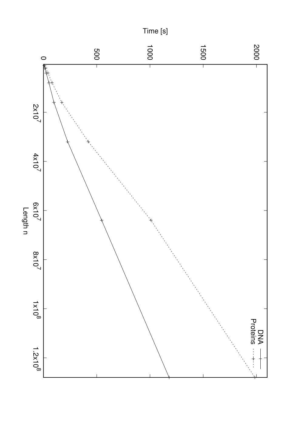
Experiment II. (Efficiency) Our task here was to establish the fact that the elapsed time of the implementation grows linearly with , the length of the input sequence. As input datasets, for this experiment, we used synthetic DNA () and proteins () sequences ranging from to M (Million letters). For each sequence we used a constant value of . The results are plotted in Fig. 3. It becomes evident from the results that the elapsed time of the program grows linearly with . The longer time required for the proteins sequences compared to the DNA sequences for increasing is explained by the dependence of the time required to answer queries of the from on the size of the alphabet ( vs. ) in the implementation of the compressed suffix tree we used.
Experiment III. (Real Application) Here we proceed to the examination of seven collections of Conserved Non-coding Elements (CNEs) obtained through multiple sequence alignment between the human and other genomes. Despite being located at the non-coding part of genomes, CNEs can be extremely conserved on the sequence level across organisms. Their genesis, functions and evolutionary dynamics still remain enigmatic [16, 13]. The detailed description of how those CNEs were identified can be found in [17]. For each CNE of these datasets, a sequence stretch (surrogate sequence) of non-coding DNA of equal length and equal GC content was taken at random from the repeat-masked human genome. The CNEs of each collection were concatenated into a single long sequence and the same procedure was followed for the corresponding surrogates. We have determined through the proposed algorithm the overabundant words for (decamers) and for these fourteen datasets and the results are presented in Table 2. Likewise, in Table 3, we show all overabundant words (i.e. ) for .
| CNEs | CNEs | CNEs | CNEs | CNEs | Mammalian | Amniotic | |
| 75-80 | 80-85 | 85-90 | 90-95 | 95-100 | |||
| Surr | 1,144 | 718 | 473 | 297 | 469 | 15,470 | 2,874 |
| CNEs | 331 | 181 | 100 | 59 | 71 | 491 | 149 |
| Ratio | 3.46 | 3.97 | 4.73 | 5.03 | 6.61 | 31.51 | 19.29 |
| CNEs | CNEs | CNEs | CNEs | CNEs | Mammalian | Amniotic | |
| 75-80 | 80-85 | 85-90 | 90-95 | 95-100 | |||
| Surr | 5,925 | 3,798 | 2,770 | 1,948 | 2,405 | 69,022 | 12,913 |
| CNEs | 1,373 | 778 | 512 | 390 | 403 | 7,549 | 1,401 |
| Ratio | 4.32 | 4.88 | 5.41 | 4.99 | 5.97 | 9.14 | 9.22 |
The first five CNE collections have been composed through multiple sequence alignment of the same set of genomes (human vs. chicken; mapped on the human genome) and they differ only in the thresholds of sequence similarity applied between the considered genomes: from 75% to 80% (the least conserved CNEs, which thus are expected to serve less demanding functional roles) to 95–100% which represent the extremely conserved non-coding elements (UCNEs or CNEs 95–100) [17]. The remaining two collections have been composed under different constraints and have been derived after alignment of Mammalian and Amniotic genomes. In Tables 2 and 3, the last line shows the ratios formed by the numbers of overabundant words of each concatenate of surrogates divided by the numbers of overabundant words of the corresponding CNE dataset. Two immediate results stem from inspection of Tables 2 and 3:
- 1.
In all cases, the number of overabundant words from the surrogate concatenate of sequences far exceeds the corresponding number derived from the CNE dataset.
- 2.
In the case of datasets with increasing degree of similarity between aligned genomes (from 75-80 to 95-100), the ratios of the numbers of overabundant words show a clear, increasing trend.
Both these findings can be understood on the basis of the difference in functionality between CNE and surrogate datasets. As we briefly describe in Section 1, this systematic difference (finding 1 above) is expected on the basis of the self-enhancing elongation of relatively long homonucleotide tracts [14, 15], which occurs mainly in the non-constrained parts of the genome, here the surrogate datasets. Moreover, finding 2 corroborates the proposed mechanism of overabundance, as in CNE datasets 1-5 depletion in overabundant words quantitatively follows the degree of sequence conservation. Inspection of the individual overabundant words found in the surrogate datasets verifies that they largely consist of short repeats of the types described in [14] and in [15]. There is an analogy of this finding with a corresponding one, concerning the occurrence of avoided words in the same sequence sets, which was described in [1].
6 Final Remarks
References
- [1] Yannis Almirantis, Panagiotis Charalampopoulos, Jia Gao, Costas S. Iliopoulos, Manal Mohamed, Solon P. Pissis, and Dimitris Polychronopoulos. On avoided words, absent words, and their application to biological sequence analysis. Algorithms for Molecular Biology, 12(1):5, 2017.
- [2] Alberto Apostolico, Mary Ellen Bock, and Stefano Lonardi. Monotony of surprise and large-scale quest for unusual words. Journal of Computational Biology, 10(3-4):283–311, 2003.
- [3] Alberto Apostolico, Mary Ellen Bock, Stefano Lonardi, and Xuyan Xu. Efficient detection of unusual words. Journal of Computational Biology, 7(1-2):71–94, 2000.
- [4] Alberto Apostolico, Fang-Cheng Gong, and Stefano Lonardi. Verbumculus and the discovery of unusual words. Journal of Computer Science and Technology, 19(1):22–41, 2004.
- [5] Djamal Belazzougui and Fabio Cunial. Space-efficient detection of unusual words. In SPIRE, volume 9309 of LNCS, pages 222–233. Springer, 2015.
- [6] Volker Brendel, Jacques S Beckmann, and Edward N Trifonov. Linguistics of nucleotide sequences: morphology and comparison of vocabularies. Journal of Biomolecular Structure and Dynamics, 4(1):11–21, 1986.
- [7] Chris Burge, Allan M. Campbello, and Samuel Karlin. Over- and under-representation of short oligonucleotides in DNA sequences. Proc Natl Acad Sci USA, 89(4):1358–1362, 1992.
- [8] Maxime Crochemore, Christophe Hancart, and Thierry Lecroq. Algorithms on strings. 2007.
- [9] Alain Denise, Mireille Régnier, and Mathias Vandenbogaert. Assessing the statistical significance of overrepresented oligonucleotides. In WABI, volume 2149 of LNCS, pages 85–97. Springer Berlin Heidelberg, 2001.
- [10] Martin Farach. Optimal suffix tree construction with large alphabets. In FOCS, pages 137–143. IEEE, 1997.
- [11] Mikhail S. Gelfand and Eugene V. Koonin. Avoidance of palindromic words in bacterial and archaeal genomes: a close connection with restriction enzymes. Nucleic Acids Research, 25(12):2430–2439, 1997.
- [12] Simon Gog, Timo Beller, Alistair Moffat, and Matthias Petri. From theory to practice: Plug and play with succinct data structures. In SEA, volume 8504 of LNCS, pages 326–337. Springer, 2014.
- [13] Nathan Harmston, Anja Barešić, and Boris Lenhard. The mystery of extreme non-coding conservation. Phil. Trans. R. Soc. B, 368(1632):20130021, 2013.
- [14] Suzanne E. Hile and Kristin A. Eckert. Positive correlation between DNA polymerase -primase pausing and mutagenesis within polypyrimidine/polypurine microsatellite sequences. Journal of Molecular Biology, 335(3):745–759, 2004.
- [15] G. Levinson and G. A. Gutman. Slipped-strand mispairing: a major mechanism for DNA sequence evolution. Molecular Biology and Evolution, 4(3):203–221, 1987.
- [16] Dimitris Polychronopoulos, Diamantis Sellis, and Yannis Almirantis. Conserved noncoding elements follow power-law-like distributions in several genomes as a result of genome dynamics. PloS One, 9(5):e95437, 2014.
- [17] Dimitris Polychronopoulos, Emanuel Weitschek, Slavica Dimitrieva, Philipp Bucher, Giovanni Felici, and Yannis Almirantis. Classification of selectively constrained DNA elements using feature vectors and rule-based classifiers. Genomics, 104(2):79–86, 2014.
- [18] Ivan Rusinov, Anna Ershova, Anna Karyagina, Sergey Spirin, and Andrei Alexeevski. Lifespan of restriction-modification systems critically affects avoidance of their recognition sites in host genomes. BMC Genomics, 16(1):1, 2015.