Phase structure of NJL model with weak renormalization group

The Lagrangian of the NJL model with one flavor is given in Eq. (I). Since in this paper we would like to investigate the fundamental behavior of the D$\chi$SB by using the weak RG, we consider the following simplified NJL model with one flavor in four dimension Euclidean space:

$\displaystyle S_{\rm NJL}=\int\text{d}^{4}x\left[\bar{\psi}{\vtop{\halign{#\cr\hfil/\hfil\crcr$\partial$\crcr}}}\psi-\frac{G_{0}}{2}(\bar{\psi}\psi)^{2}\right],$

where we assume that the quark fields have the degree of freedom of color, $N_{\text{c}}$. Since the pseudo-scalar operator $(\bar{\psi}i\gamma^{5}\psi)^{2}$ is not introduced, this action has no continuous chiral symmetry. Instead, it is invariant under the discrete type transformation,

$\displaystyle\psi$

$\displaystyle\to\gamma^{5}\psi,$

$\displaystyle\bar{\psi}$

$\displaystyle\to-\bar{\psi}\gamma^{5},$

(5)

which forbids the operators with negative power of $\bar{\psi}\psi$. Hence, the mass term of fermion $m\bar{\psi}\psi$ does not appear in the action. This model describes that the chiral symmetry breaks down due to the strong four-Fermi interaction and the non-trivial vacuum, i.e., the non-zero chiral condensate $\langle\bar{\psi}\psi\rangle\neq 0$, is realized. In this vacuum, the fermion obtains the dynamical mass which is proportional to the chiral condensate. It should be noted that we do not really work for the discrete chiral symmetric model with only scalar four-fermi interactions. Starting with the continuous chiral symmetric model with scalar and pseudo-scalar four-fermi interactions together, we define the renormalized fermionic interactions expressed in terms of scalar bilinear $\bar{\psi}\psi$ and pseudo-scalar bilinear $\bar{\psi}i\gamma_{5}\psi$ operators. The renormalized interactions have the same continuous chiral symmetry, since the RG beta functions are set to respect the symmetry.

After integrating the RG equation to the infrared end, we investigate the free energy (vacuum amplitude) as a function of scalar and pseudo-scalar source fields. The free energy is readily obtained making use of the translational invariance feature of our beta functions. By the Legendre transformation in a usual way, we define the effective potential as a function of $\sigma=\langle\bar{\psi}\psi\rangle$ and $\pi=\langle\bar{\psi}i\gamma_{5}\psi\rangle$, which has the same chiral symmetric form, i.e., it is a function of $\sigma^{2}+\pi^{2}$.

Therefore only a section of the effective potential where $\pi=0$ is sufficient to get the radial profile of it. It is shown straightforwardly that this section does not depend on the coupling constant of elementary pseudo-scalar interactions in the bare Lagrangian. Then we set the vanishing pseudo-scalar coupling constant. This is our strategy of model set up, which gives the shortest way of evaluating the effective potential profile.³³ 3 We comment on the finite number flavor case. In a general flavor case, the chiral symmetry is given as $\text{SU}\!\left(N_{\text{f}}\right)_{V}\times\text{SU}\!\left(N_{\text{f}}\right)_{A}\times\text{U}\!\left(1\right)_{V}\times\text{U}\!\left(1\right)_{A}$. $\text{U}\!\left(1\right)_{A}$ symmetry is broken by the chiral anomaly. This effective is described by the ’t Hooft–Kobayashi–Maskawa term [38, 39, 40] within the effective model approach. Since this term with $N_{\text{f}}=2$ is given as the four-Fermi interaction, we would expect no crucial difference from the present setup. In contrast, in the $N_{\text{f}}=3$ (or $2+1$) case, ’t Hooft–Kobayashi–Maskawa term is given by the six-Fermi interaction. Although the anomaly effect on the chiral phase transition is investigated in several literatures, e.g. [41, 42, 43], it might depend on chiral effective models. We should, however, take account of the pseudo-scalar operator to calculate, for example, critical exponents, which are sensitive to the difference of the discrete and continuous symmetries.

We introduce the FRG to investigate the D$\chi$SB in the NJL model. Now, we briefly explain its idea and derivation. Let us consider the bare action $S[\phi;\Lambda_{0}]$ and the path integral,

$\displaystyle Z=\int\mathcal{D}\phi\,{\rm e}^{-S[\phi;\Lambda_{0}]}.$

(6)

This integration can be interpreted as the summation of the quantum fluctuations with the momentum $0<|p|<\Lambda_{0}$. In the FRG, the path integral is evaluated by integrating out the quantum fluctuation with the higher momentum $\Lambda<|p|<\Lambda_{0}$, namely,

$\displaystyle Z=\int\mathcal{D}\phi_{<}\mathcal{D}\phi_{>}\,{\rm e}^{-S[\phi_{<}+\phi_{>};\Lambda_{0}]}=\int\mathcal{D}\phi_{<}\,{\rm e}^{-S_{\rm eff}[\phi_{<};\Lambda]},$

(7)

where we divided the field $\phi\!\left(p\right)$ into the higher momentum mode $\phi_{>}\!\left(p\right)$ with $\Lambda<|p|<\Lambda_{0}$ and the lower momentum mode $\phi_{<}\!\left(p\right)$ with $0<|p|<\Lambda$. The action $S_{\rm eff}[\phi_{<};\Lambda]$ is called the Wilsonian effective action and is defined by the lower momentum mode. The FRG describes the change from the bare action $S[\phi;\Lambda_{0}]$ to the effective action $S_{\rm eff}[\phi_{<};0]$ through integrating the shell momentum $\Lambda-\delta\Lambda<|p|<\Lambda$, which is the so-called coarse graining. This step is formulated as a functional differential equation, and solving this equation is equivalent to evaluating the path integral (6). In this paper, we employ the Wegner-Houghton (WH) equation [44],

$\displaystyle\frac{\text{d}S_{\rm eff}}{\text{d}t}=-\frac{1}{2}\int_{\rm shell}\frac{\text{d}^{d}p}{(2\pi)^{d}}\left\{\frac{\delta S_{\rm eff}}{\delta\phi_{p}}\left(\frac{\delta^{2}S_{\rm eff}}{\delta\phi_{p}\delta\phi_{-p}}\right)^{-1}\frac{\delta S_{\rm eff}}{\delta\phi_{-p}}-{\rm str}\log\!\left(\frac{\overrightarrow{\delta}}{\delta\phi_{p}}S_{\rm eff}\frac{\overleftarrow{\delta}}{\delta\phi_{-p}}\right)\right\},$

(8)

where $\phi_{p}:=\phi\!\left(p\right)$ and we introduced the dimensionless scale parameter,

$\displaystyle t:=\log\!\left(\Lambda_{0}/\Lambda\right).$

(9)

It is rewritten as $\Lambda=\Lambda_{0}{\rm e}^{-t}$, and then the increasing $t$ corresponds to the decreasing the cutoff $\Lambda$. Since the two point function $\frac{\overrightarrow{\delta}}{\delta\phi_{p}}S_{\rm eff}\frac{\overleftarrow{\delta}}{\delta\phi_{-p}}$ is generally given as the supermatrix in field space, “str” denotes taking the trace for the supermatrix; see [45, 46] for the treatments of the supermatrix and its manipulations. For details of derivation of the WH equation, see e.g. [45].⁴⁴ 4 The WH equation is also obtained from the sharp cutoff limit of the Plochinski equation [47, 48] The Wilsonian effective action is generally spanned by an infinite number of effective operators generated by the interactions in the bare action. Note that symmetries which the bare action has are not broken through the shell momentum integral, hence, the generated effective operators respect their symmetries.

Although the WH equation (8) itself is exact, we cannot solve it without some approximations. That is, we have to restrict the theory space of the Wilsonian effective action to its subspace. We give the following action as the approximated Wilsonian effective action for the NJL model (II.1):

$\displaystyle S_{\rm eff}[\psi,\bar{\psi};\Lambda]=\int\text{d}^{4}x\left[\bar{\psi}{\vtop{\halign{#\cr\hfil/\hfil\crcr$\partial$\crcr}}}\psi-V\!\left(\bar{\psi}\psi;\Lambda\right)\right].$

If the effective potential is expanded into the polynomials of $\bar{\psi}\psi$, we have

$\displaystyle V\!\left(\bar{\psi}\psi;\Lambda\right)=\frac{G_{\Lambda}}{2}(\bar{\psi}\psi)^{2}+\frac{G_{4,\Lambda}}{4}(\bar{\psi}\psi)^{4}+\cdots.$

(12)

We call this potential the “fermionic” effective potential. As mentioned above, the odd powers of $\bar{\psi}\psi$ is not generated due to the (discrete) chiral symmetry. The potential at the initial scale $\Lambda_{0}$ is given by

$\displaystyle V\!\left(\bar{\psi}\psi;\Lambda_{0}\right)=\frac{G_{0}}{2}\left(\bar{\psi}\psi\right)^{2},$

(13)

that is, $G_{\Lambda_{0}}\equiv G_{0}$ and other effective coupling constants vanish. Hereafter, we will use the notations $\sigma:=\bar{\psi}\psi$. Note that the variable $\sigma$ is not an auxiliary field, accordingly its derivatives with respect to $\psi$ and $\bar{\psi}$ are given as

$\displaystyle\sigma\,\frac{\overleftarrow{\partial}}{\partial\psi}$

$\displaystyle=\bar{\psi},$

$\displaystyle\frac{\overrightarrow{\partial}}{\partial\bar{\psi}}\,\sigma$

$\displaystyle=\psi.$

(14)

We will discuss the chiral phase transition by the effects of temperature and density in the next section. For this purpose, the density operator $\int\text{d}^{4}x\,\mu\bar{\psi}\gamma_{0}\psi$ should be introduced in the bare action (II.1) and the Wilsonian effective action (II.2).⁵⁵ 5 We assume that the chemical potential $\mu$ is not corrected by quantum fluctuations. Moreover, the momentum in the time direction $p_{0}$ is replaced with the Matsubara frequency $\omega_{n}$ and its integration becomes the Matsubara summation. It is complicated to evaluate the shell momentum integral for four dimension momentum. To avoid it, we insert the cutoff $\Lambda$ into the momentum in the spatial direction. Then the shell momentum integral becomes

$\displaystyle\int_{\rm shell}\frac{\text{d}^{4}p}{(2\pi)^{4}}=T\displaystyle\sum_{n=-\infty}^{\infty}\int\frac{\text{d}^{3}p}{(2\pi)^{3}}\,\Lambda\,\delta\!\left(|\vec{p}|-\Lambda\right).$

(15)

The RG equation for the effective potential is given by

$\displaystyle\partial_{t}V\!\left(\sigma;t\right)=\frac{\Lambda^{3}}{\pi^{2}}\bigg[E+T\log\!\left(1+{\rm e}^{-\beta(E-\mu)}\right)+T\log\!\left(1+{\rm e}^{-\beta(E+\mu)}\right)\bigg],$

(16)

where $\beta=1/T$, $E:=\sqrt{\Lambda^{2}+M^{2}}$ and $M:=\partial_{\sigma}V$. We show the explicit derivation of the RG equation in the appendix A. Note that the large-$N$ approximation ($N_{\text{c}}\to\infty$) and the uniform $\bar{\psi}\psi$ approximation were employed in order to obtain Eq. (16). The function $M$ corresponds to the dynamical mass of quark. We here call it the mass function.

Here, we revisit the NJL model at vanishing temperature and density. The RG equation (16) at zero temperature and zero density becomes

$\displaystyle\partial_{t}V\!\left(\sigma;t\right)=\frac{\Lambda^{3}}{\pi^{2}}\sqrt{\Lambda^{2}+\left(\partial_{\sigma}V\right)^{2}}.$

(17)

Using the expansion of the effective potential given in Eq. (12), we obtain the RG equations of each coupling constant. In particular, the RG equation of the four-Fermi coupling constant is given by

$\displaystyle\partial_{t}G=\frac{G^{2}\Lambda^{2}}{\pi^{2}}.$

(18)

If we use the dimensionless rescaled coupling constant $\tilde{G}:=G\Lambda^{2}/2\pi^{2}$, it becomes

$\displaystyle\partial_{t}\tilde{G}=-2\tilde{G}+2\tilde{G}^{2}.$

(19)

Obviously, this equation has the fixed point $\tilde{G}_{\rm c}=1$ and yields the blow-up solution,

$\displaystyle\tilde{G}\!\left(t\right)=\frac{\tilde{G}_{\rm c}\tilde{G}_{0}}{\tilde{G}_{0}-(\tilde{G}_{0}-\tilde{G}_{\rm c}){\rm e}^{2t}},$

(20)

for the initial value $\tilde{G}_{0}>\tilde{G}_{\rm c}$. We see the critical scale at which the denominator becomes zero,

$\displaystyle t_{\rm c}=\frac{1}{2}\log\!\left(\frac{\tilde{G}_{0}}{\tilde{G}_{0}-\tilde{G}_{\rm c}}\right).$

(21)

The divergence of $\tilde{G}$ itself is physically relevant since it corresponds to the chiral fluctuation $\tilde{G}\sim\langle(\bar{\psi}\psi)^{2}\rangle$. Thus, the divergence is the signal of the second order phase transition. However, the divergence disturbs solving the RG equation up to the infrared (IR) scale $\Lambda\to 0$. Since the four-Fermi coupling constant is lowest order of the effective potential (12), the effective potential becomes non-differentiable at its origin $V\!\left(\sigma=0\right)$ due to the singularity of the four-Fermi coupling constant. In other words, the derivative $\partial_{\sigma}V$ cannot be defined after the critical scale $t_{\rm c}$.

We see in the next section that the weak solution method [37] allows us to analyze the D$\chi$SB without introducing the auxiliary field and to investigate the chiral first-order phase transition.

As discussed in the previous section, the RG equation for the effective potential becomes singular when the D$\chi$SB occurs. In [37], it was shown that the weak solution method is valid for overcoming the singularity of this system. Here, we briefly review basic notions of the weak solution method and show the weak RG equation for Eq. (16).

The RG equation (16) is given as the partial differential equation,

$\displaystyle\partial_{t}V\!\left(\sigma;t\right)=-F\!\left(M\!\left(\sigma;t\right),\sigma;t\right),$

(22)

where $F\!\left(M,\sigma;t\right)$ is the beta function with a negative sign. Differentiating the both sides of RG equation with respect to $\sigma$, we obtain

$\displaystyle\partial_{t}M\!\left(\sigma;t\right)+\partial_{\sigma}F\!\left(M\!\left(\sigma;t\right),\sigma;t\right)=0.$

(23)

Let us now call this equation the “strong” RG equation in order to compare with the “weak” RG equation introduced below.

Here, we introduce a test function $\varphi\!\left(\sigma;t\right)$ which is smooth and converges to zero for both infinite $t$ and $\sigma$: $\varphi\!\left(\pm\infty;t\right)=\varphi\!\left(\sigma;\infty\right)=0$. Integrating Eq. (23) multiplied by this function, we have

$\displaystyle\int^{\infty}_{0}\text{d}t\int^{\infty}_{-\infty}\text{d}\sigma\left(\partial_{t}M+\partial_{\sigma}F\right)\varphi\!\left(\sigma;t\right)=0.$

(24)

By utilizing the integration by parts, it becomes

$\displaystyle\int^{\infty}_{0}\text{d}t\int^{\infty}_{-\infty}\text{d}\sigma\left(M\frac{\partial\varphi}{\partial t}+F\frac{\partial\varphi}{\partial\sigma}\right)+\int^{\infty}_{-\infty}\text{d}\sigma\,(M\,\varphi)|_{t=0}=0.$

(25)

We call the RG equation (25) “weak RG equation”, and its solution is called “weak solution”. The derivatives with respect to $t$ and $\sigma$ move from the mass function and the beta function to the test function. Hence, $M\!\left(\sigma;t\right)$ given as a solution of the weak RG equation (25) can have an arbitrary number of singularities at any point on the $\sigma$–$t$ plane.

The RG equation of the mass function (23) is given as a partial differential equation. Here, we introduce the method of characteristics which reduces from the partial differential equation to the system of ordinary differential equations. The method of characteristics allows us to numerically solve the RG equation using e.g., the Runge-Kutta method and the finite-difference methods.

Let us consider a curved surface $M\!\left(\sigma;t\right)$ in the $\sigma$–$t$–$z$ space and rewrite the RG equation (23) as

$\displaystyle\begin{pmatrix}\partial_{M}F&1&0\end{pmatrix}\begin{pmatrix}\partial_{\sigma}M\\ \partial_{t}M\\ -1\end{pmatrix}=0,$

(26)

where we used $\partial_{\sigma}F=(\partial_{M}F)(\partial_{\sigma}M)$. The infinitesimal displacement vector $(\text{d}\sigma,\text{d}t,\text{d}M)$ is a tangent vector for a point $(\sigma,t,M)$ on the curved surface $M\!\left(\sigma;t\right)$, and satisfies

$\displaystyle\begin{pmatrix}\text{d}\sigma&\text{d}t&\text{d}M\end{pmatrix}\begin{pmatrix}\partial_{\sigma}M\\ \partial_{t}M\\ -1\end{pmatrix}=0,$

(27)

since the total derivative of $M$ is given by $\text{d}M=\partial_{\sigma}M\,\text{d}\sigma+\partial_{t}M\,\text{d}t$. Thus, the vector $(\partial_{\sigma}M~\partial_{t}M\,-1)^{\rm T}$ is orthogonal to $(\text{d}\sigma~\text{d}t~\text{d}M)$, and we find that the vector $(\partial_{M}F~1~0)$ is also the tangent vector for a point on the curved surface $M\!\left(\sigma;t\right)$. Taking $(\text{d}\sigma~\text{d}t~\text{d}M)$ as the vector being proportional to $(\partial_{M}F~1~0)$, we have

		$\displaystyle\frac{\text{d}\sigma\!\left(s\right)}{\text{d}s}=\frac{\partial F}{\partial M},$		(28)
		$\displaystyle\frac{\text{d}t\!\left(s\right)}{\text{d}s}=1,$		(29)
		$\displaystyle\frac{\text{d}M\!\left(\sigma,s\right)}{\text{d}s}=0,$		(30)

where we introduced an infinitesimal parameter $\text{d}s$ as a proportionality constant. The solutions $\left(\sigma\!\left(s\right),t\!\left(s\right),M\!\left(s\right)\right)$ of the system of ordinary differential equations with each initial conditions are called characteristics. Since the solution of Eq. (29) is simply $t=s$, we can replace from $s$ to $t$ in Eqs. (28) and (30).

The fermionic effective potential $V$ can be evaluated within the method of characteristics. Considering $V$ on the characteristics, we obtain

	$\displaystyle\frac{\text{d}V\!\left(s\right)}{\text{d}s}$	$\displaystyle=\frac{\partial V\!\left(\sigma;s\right)}{\partial\sigma}\frac{\text{d}\sigma\!\left(s\right)}{\partial s}+\frac{\partial V\!\left(\sigma;s\right)}{\partial s}$
		$\displaystyle=M\frac{\partial F}{\partial M}-F,$		(31)

where we used Eqs. (23), (28) and $M=\partial_{\sigma}V$.

To summarize, we have the following coupled equations for the present system:

$\displaystyle\frac{\text{d}\sigma\!\left(t\right)}{\text{d}t}=\frac{\partial F}{\partial M},$

$\displaystyle\frac{\text{d}M\!\left(\sigma,t\right)}{\text{d}t}=0,$

$\displaystyle\frac{\text{d}V\!\left(t\right)}{\text{d}t}=M\frac{\partial F}{\partial M}-F.$

(32)

Actually, these equations are independent of each other, therefore, their solutions are given by

		$\displaystyle M\!\left(\sigma\!\left(t\right);t\right)=M\!\left(\sigma_{0};0\right)=:M_{0},$		(33)
		$\displaystyle\sigma\!\left(t\right)=\sigma_{0}+\int^{t}_{0}\text{d}\tau\,\partial_{M}F\!\left(M_{0};\tau\right),$		(34)
		$\displaystyle V\!\left(\sigma;t\right)=V\!\left(\sigma_{0};0\right)+\int^{t}_{0}\text{d}\tau\,\left.\left[M\frac{\partial F}{\partial M}-F\right]\right|_{M=M_{0}},$		(35)

where $\sigma_{0}:=\sigma\!\left(0\right)$. Note here that $F\!\left(M,\sigma;t\right)$ given in the right-hand side of Eq. (16) (with negative sign) does not explicitly depend on $\sigma$; $F\!\left(M,\sigma;t\right)\equiv F\!\left(M;t\right)$. We also note that this simplification happens in the NJL model with a certain approximation. Although for more general cases such as QCD, we have to solve the system of ordinary differential equations for a given system, solving it is easier than the case of the partial differential equation.

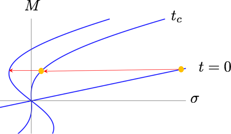
A schematic figure for the evolution of the mass function described by Eqs. (33)–(35) is shown in Fig. 1. Note that for a fixed $M_{0}>0$, $\sigma$ described by Eq. (34) moves towards the left-hand side since $\partial^{2}F/\partial M^{2}<0$ for Eq. (16) is satisfied; see the appendix B. The system of ordinary differential equations (33)–(35) does not yield any singularity. Instead, as a schematic figure shown in Fig. 2, after the critical scale $t_{c}$, the mass function becomes a multi-valued function around a value $\sigma^{*}$, at which the fermionic effective potential becomes the swallowtail form (the right-hand side of Fig. 2). However, the solution of the fermionic potential and the mass function after the D$\chi$SB have to be a single-valued function of $\sigma$ since there should exist only one physical vacuum. To uniquely determine the physical vacuum, we give the Rankine–Hugoniot condition in the next subsection.

To uniquely determine the weak solution from Eq. (25) (or equivalently Eq. (32)), we give a condition called the Rankine–Hugoniot (RH) condition. This condition is derived from the definition of the weak solution and reads

$\displaystyle\frac{\text{d}\sigma^{*}\!\left(t\right)}{\text{d}t}=\frac{F\!\left(M\!\left(\sigma_{+}^{*}\!\left(t\right)\right);t\right)-F\!\left(M\!\left(\sigma_{-}^{*}\!\left(t\right);t\right)\right)}{M\!\left(\sigma_{+}^{*}\!\left(t\right);t\right)-M\!\left(\sigma_{-}^{*}\!\left(t\right);t\right)},$

(36)

where $\sigma^{*}\!\left(t\right)$ is a discontinuity point, and $\sigma_{+}^{*}$ and $\sigma_{-}^{*}$ denote closing to the point $\sigma^{*}$ from the right-hand side ($+$) and the left-hand side ($-$), respectively (see Fig. 2). This condition describes the evolution of $\sigma^{*}\!\left(t\right)$ and implies geometrically the differential-area invariance, namely,

$\displaystyle S_{A}\!\left(t\right)-S_{B}\!\left(t\right)={\rm constant}.$

(37)

In the present case, since at the critical scale $t=t_{\text{c}}$, $S_{A}\!\left(t_{\text{c}}\right)=S_{B}\!\left(t_{\text{c}}\right)=0$ is satisfied, the constant value in Eq. (37) vanishes, and then $S_{A}\!\left(t\right)=S_{B}\!\left(t\right)$. In Fig. 2, the RH condition means that the vertical line (gray line) is defined such that the equal area rule $S_{A}\!\left(t\right)=S_{B}\!\left(t\right)$ is satisfied and the dotted line is ruled out as the solution. The weak solution being the solution of Eq. (25) with the RH condition is given by the solid line with a discontinuity at $\sigma^{*}$. The discontinuity determined by the RH condition is called ‘‘shock’’.⁶⁶ 6 The terminology comes from the “shock wave” in gas dynamics.

As an example, the evolution of the mass function at vanishing temperature and density is shown in Fig. 3, where the dimensionless mass function $\tilde{M}=M/\Lambda_{0}$ and the dimensionless field $\tilde{\sigma}=\sigma/\Lambda_{0}$ are defined; see Eqs. (52) and (53) in the section IV. At the critical scale $t_{c}$, the slope of the mass function at $\tilde{\sigma}=0$ becomes infinity, which corresponds to the divergence of the four-fermi coupling constant. After $t_{c}$, the solution of the mass function becomes the multi-valued function. Applying the RH condition, the solution is uniquely determined; see the right-hand panel of Fig. 3. Next, let us consider the case at zero temperature and finite density. The evolution of the mass function in this case is shown in Fig. 4. We see that two singularities arise at the non-zero field values, $\tilde{\sigma}\neq 0$. They move towards the origin $\tilde{\sigma}=0$ and eventually merge with lowering the scale $t$. For such a behavior of the mass function, we observe the first-order phase transition as will be seen in the next section.

The mass function given as the weak solution satisfies

$\displaystyle M\!\left(\sigma\!\left(t\right);t\right)=-M\!\left(-\sigma\!\left(t\right);t\right),$

(38)

since it reflects the chiral transformation $\sigma\to-\sigma$. Then, the dynamical mass is given by

$\displaystyle M_{\text{phys}}=\lim_{\sigma\to 0_{+}}M\!\left(\sigma;\infty\right)=-\lim_{\sigma\to 0_{-}}M\!\left(\sigma;\infty\right).$

(39)

To summarize so far, the multi-valued mass function as a solution of the characteristics (33)–(35) is uniquely determined for any field value of $\sigma$ by the RH condition. Instead, the mass function with the RH condition has the discontinuities. Such a solution is defined mathematically as the weak solution of Eq. (25) in which the mass function and its beta function are not differentiated by $t$ and $\sigma$. The physical dynamical mass is given by Eq. (39).

Finally, we comment on the Legendre effective potential and its convexity and concavity. Let us start with defining the generating functional for the connected Green function,

$\displaystyle W\!\left(j;t\right):=V\!\left(\sigma=0;t;j\right).$

(40)

Here, the initial condition for the fermionic potential is given by

$\displaystyle V\!\left(\sigma;t=0;j\right)=\frac{G_{0}}{2}\sigma^{2}+j\sigma,$

(41)

where the last term is the source term. From the Legendre transformation of Eq. (40), we can define the Legendre effective potential,

$\displaystyle V_{\rm L}\!\left(\phi;t\right):=j\,\phi\!\left(j;t\right)-W\!\left(j;t\right).$

(42)

This potential is a function of the chiral condensate given by

$\displaystyle\phi\!\left(j;t\right):=\frac{\partial W\!\left(j;t\right)}{\partial j}=\langle\bar{\psi}\psi\rangle_{j}.$

(43)

Note that the source $j$ is regarded as a function of $\phi$. It is known that the Legendre effective potential $V_{\rm L}$ becomes the convex form [49, 50, 51, 52]. The weak solution method automatically gives us the convex Legendre effective potential as the convex envelope of the nonconvex function obtained from the solution of characteristic equations (33)–(35). See discussions in [37] on its proof.

We discuss the RG flow of the four-Fermi coupling constant in view of the weak solution. Since the mass function $M\!\left(\sigma;t\right)$ is given by

$\displaystyle M\!\left(\sigma;t\right)=\partial_{\sigma}V\!\left(\sigma;t\right)=G_{\Lambda}\sigma+\cdots,$

(44)

the behavior of the origin of $M\!\left(\sigma;t\right)$ is described by the four-Fermi coupling constant. At the critical scale $t_{\rm c}$ at which the four-Fermi coupling constant diverges, the slope of the mass function at $\sigma=0$ becomes infinity; see the orange line in Fig. 3. After the critical scale, it becomes negative whereas the RG flow of the four-Fermi coupling constant given by Eq. (19) cannot be evaluated due to the divergence. We have seen in the previous section that in the weak solution method with the RH condition, the mass function with the discontinuities is defined mathematically and uniquely determined for any field value of $\sigma$. Note that in the case where the first-order phase transition takes place, the slope of the mass function at the origin does not become infinity; see Fig. 4. That is, the RG flow of the four-Fermi coupling constant does not diverge at any scale.

Next, we discuss the relation between the inverse four-Fermi coupling constant $g:=1/G_{\Lambda}$ and the Legendre effective potential $V_{\rm L}$. We start with the well-known relation,

$\displaystyle-\frac{\partial^{2}W}{\partial j^{2}}\cdot\frac{\partial^{2}V_{\rm L}}{\partial\phi^{2}}=1,$

(45)

where $W\!\left(j;t\right)$ is given in Eq. (40). The second derivative of $W$ with respect to $j$ corresponds to the susceptibility:

$\displaystyle\chi\!\left(j\right):=\frac{\partial\langle\bar{\psi}\psi\rangle_{j}}{\partial j}=-\frac{\partial^{2}W}{\partial j^{2}}=\langle(\bar{\psi}\psi)^{2}\rangle_{j}-(\langle\bar{\psi}\psi\rangle_{j})^{2}.$

(46)

Together with Eq. (45), we obtain

$\displaystyle\frac{\partial^{2}V_{\rm L}\!\left(\phi;t\right)}{\partial\phi^{2}}=\frac{1}{\chi\!\left(j\right)}.$

(47)

When the second-order phase transition occurs, the susceptibility diverges: $\chi\to\infty$. That is, the left-hand side $\frac{\partial^{2}V_{\rm L}\!\left(\phi;t\right)}{\partial\phi^{2}}$ vanishes at the critical scale $t=t_{\rm c}$. More explicitly, we see

$\displaystyle\frac{\partial^{2}V_{\rm L}\!\left(\phi;t\right)}{\partial\phi^{2}}=m^{2}+\lambda\phi^{2}+\cdots.$

(48)

At the origin of $V_{\rm L}$, the mass-squared $m^{2}$, i.e. the curvature of $V_{\rm L}$, corresponds to the inverse susceptibility $1/\chi$. The divergence of $\chi$ means the vanishing mass-squared $m^{2}=0$. As mentioned in the section II, the four-Fermi coupling constant corresponds to the chiral susceptibility:

$\displaystyle G_{\Lambda}=\frac{1}{2}\left.\frac{\partial^{2}W\!\left(j\right)}{\partial j^{2}}\right|_{j=0}+G_{\Lambda_{0}}.$

(49)

Then, the divergence of $G_{\Lambda}$ is the signal of the second-order phase transition, and we see that the inverse four-Fermi coupling constant corresponds to the curvature at the origin of the Legendre effective potential:

$\displaystyle m^{2}=\frac{1}{G_{\Lambda}}.$

(50)

The RG flow of the dimensionless rescaled inverse four-Fermi coupling constant $\tilde{\kappa}=\tilde{G}^{-1}=2\pi^{2}/(G_{\Lambda}\Lambda^{2})$ is given by

$\displaystyle\tilde{\kappa}\!\left(t\right)=1-(1-\tilde{\kappa}_{0}){\rm e}^{2t},$

(51)

where $\tilde{\kappa}_{0}$ is the initial value of $\tilde{\kappa}$ at the initial scale $t=0$. For $\tilde{\kappa}_{0}<1$, $\kappa\!\left(t\right)$ becomes negative after $t=t_{\rm c}$ at which $\tilde{\kappa}\!\left(t_{\rm c}\right)=0$. Thus, from the relation (50), one can see that the negative $\tilde{\kappa}$ corresponds to the negative curvature at the origin of the Legendre effective action. The negative curvature at the origin means that the non-vanishing vacuum $\langle\phi\rangle=\langle\bar{\psi}\psi\rangle\neq 0$ exists. However, one cannot evaluate the value of the chiral condensate by only observing the divergence of the four-Fermi coupling constant in the second-order phase transition. Besides, the first-order phase transition is not captured by only looking for the behavior of the four-Fermi coupling constant.

In the next section, we analyze the weak renormalization group at finite temperature and density and show the chiral phase structures of the NJL model.

We make the dimensionless beta function of $F\!\left(\sigma;t\right)$ given in Eq. (16) at finite temperature and density:

$\displaystyle\tilde{F}\!\left(\tilde{\sigma};t\right)=-\frac{{\rm e}^{-3t}}{\pi^{2}}\bigg[{\tilde{E}}+{\tilde{T}}\log\!\left(1+{\rm e}^{-{\tilde{\beta}}({\tilde{E}}-{\tilde{\mu}})}\right)+{\tilde{T}}\log\!\left(1+{\rm e}^{-{\tilde{\beta}}({\tilde{E}}+{\tilde{\mu}})}\right)\bigg],$

(52)

where we defined the dimensionless variables,

$\displaystyle\tilde{E}$

$\displaystyle=\frac{E}{\Lambda_{0}}=\sqrt{{\rm e}^{-2t}+\tilde{M}^{2}},$

$\displaystyle\tilde{M}$

$\displaystyle=\frac{M}{\Lambda_{0}},$

$\displaystyle\tilde{\sigma}$

$\displaystyle=\frac{\sigma}{\Lambda_{0}^{3}},$

$\displaystyle\tilde{\beta}^{-1}=\tilde{T}$

$\displaystyle=\frac{T}{\Lambda_{0}},$

$\displaystyle\tilde{\mu}$

$\displaystyle=\frac{\mu}{\Lambda_{0}}.$

(53)

One obtains evolutions of the dimensionless mass function and the dimensionless effective potential by solving the dimensionless characteristic equations,

$\displaystyle\frac{\text{d}\tilde{\sigma}\!\left(t\right)}{\text{d}t}=\frac{\partial\tilde{F}}{\partial\tilde{M}},$

$\displaystyle\frac{\text{d}\tilde{M}\!\left(\tilde{\sigma},t\right)}{\text{d}t}=0,$

$\displaystyle\frac{\text{d}\tilde{V}\!\left(t\right)}{\text{d}t}=\tilde{M}\frac{\partial\tilde{F}}{\partial\tilde{M}}-\tilde{F},$

(54)

with the initial conditions at $t=0$ ($\Lambda=\Lambda_{0}$),

$\displaystyle{\tilde{V}}\!\left(\tilde{\sigma};t=0\right)$

$\displaystyle=\pi^{2}g_{0}{\tilde{\sigma}^{2}},$

$\displaystyle{\tilde{M}}\!\left(\tilde{\sigma};t=0\right)$

$\displaystyle=2\pi^{2}g_{0}{\tilde{\sigma}},$

(55)

where $g_{0}:=G_{0}\Lambda_{0}^{2}/2\pi^{2}$. Note that the critical value of $g_{0}$ at vanishing temperature and density is $g_{0}{}_{\text{c}}=1$. Hence, for $g_{0}>1$, the D$\chi$SB is observed.

Here setting $g_{0}=2$ as a benchmark point, we show the dependence of the mass function on temperature and density. First, let us consider the zero density case $\mu=0$. We show the dependence of the mass function in the IR limit $t\to\infty$ ($\Lambda\to 0$) on temperature in Fig. 5. With increasing $\tilde{T}$, the value of the mass function at $\tilde{\sigma}\to 0$ smoothly becomes smaller. This behavior corresponds to the second-order phase transition. Note that the dynamical mass is given in Eq. (39). The mass function at $\tilde{\sigma}\to 0$ vanishes at ${\tilde{T}}_{\text{c}}\simeq 0.589$ which is the critical temperature. Next, we consider the finite chemical potential and vanishing temperature case. In this case, the evolution of the mass function in the IR limit is shown in Fig. 6. We see that the slope of the origin of the mass function changes from negative to positive at $\tilde{\mu}\simeq 0.707$; see the left-hand side of Fig. 6. This means that the four-Fermi coupling constant becomes positive via the divergence, and thus the Legendre effective potential has a local minimum at its origin. Here we call this behavior the “second-order” although it does not always correspond to the phase transition. Note that there is still a non-trivial global minimum at $\tilde{\mu}\simeq 0.707$. Above $\tilde{\mu}_{\text{c}}\simeq 0.861$, the discontinuities of the mass function in the IR limit are located at non-vanishing $\sigma$. Then, when taking the limit $\sigma\to 0$, the physical dynamical mass suddenly vanishes with increasing $\tilde{\mu}$, i.e., $M\!\left(\sigma\to 0;t\to\infty;T=0,\mu<\mu_{\text{c}}\right)\neq 0\to M\!\left(\sigma\to 0;t\to\infty;T=0,\mu>\mu_{\text{c}}\right)=0$. This phase transition is of first-order. We see that the weak solution method can capture the phase transitions with both second- and first-order. In the next subsection, we show the phase diagram on the $g_{0}$–$\tilde{\mu}$–$\tilde{T}$ plane.

In Fig. 7, the chiral phase diagram on the $g_{0}$–$\tilde{\mu}$–$\tilde{T}$ plane are shown. The red line stands for the second-order phase boundary. As discussed in the section II, this boundary can be obtained by only the behavior of the four-Fermi coupling constant. The blue line corresponds to the first-order phase boundary. The biggest and smallest phase boundaries correspond to the cases of $g_{0}=2$ and $g_{0}=1.0101$, respectively. We show the phase diagram on the $\tilde{\mu}$–$\tilde{T}$ plane in Fig. 8, which is obtained by the projection from the three dimensional phase diagram of Fig. 7. A schematic figure of a phase boundary with a fixed four-Fermi coupling constant is shown in Fig. 9. Note that the region, which is surrounded by the second- and first-order phase boundaries towards the high density side, is the broken phase. As discussed in the previous subsection, although the four-Fermi coupling constant diverges at the second-order phase boundary, that is, the curvature of the origin of the effective potential becomes positive, the global minimum is still located at the non-vanishing chiral condensate. In Fig. 10, the behaviors of the critical end-point (CEP) and the second-order phase boundary at $T=0$ with varying the four-Fermi coupling constant are shown. At a finite value of the four-Fermi coupling constant $g_{0}\simeq 1.2$, they merge and the CEP vanishes.⁷⁷ 7 We see in Fig. 8 that the first-order phase boundary abruptly disappears at a certain four-Fermi coupling constant. However, the CEP should completely merge with the second-order phase boundary at $T=0$. In order to see this, we need very precise numerical calculations. Here, extrapolating the CEP towards the horizontal axis, we obtain the value of the four-Fermi coupling constant at which the critical end-point merges with the second-order phase boundary at $T=0$. The first-order phase boundary vanishes for the smaller four-Fermi coupling constant than $g_{0}\simeq 1.2$. We again emphasize that the chiral phase diagrams shown in this work are obtained by the RG equation without introducing the auxiliary field.

Here, we note the case where the finite bare mass is taken into account. In this case, we could observe the crossover for smaller chemical potential rather than the second-order phase transition. This behavior within the weak renormalization group is shown in [37].

Let us compare our results with other models and methods. We first note that as shown in Refs. [9, 53], the FRG analysis in the large-$N$ limit is equivalent to the SDE with the ladder approximation. The ladder approximated SDE is also equivalent to the MFA. Therefore, these methods yield quantitatively the same results.

We compare the present work with the other ones in the two-flavor and three-color case ($N_{\text{f}}=2$, $N_{\text{c}}=3$).⁸⁸ 8 In the present setup, there are no significant differences between one-flavor and two-flavor cases. See the comments in the footnote 3. For the mean-field analysis of the NJL model, we employ the following Lagrangian,

$\displaystyle{\mathcal{L}}_{\text{2fNJL}}=\bar{\psi}({\vtop{\halign{#\cr\hfil/\hfil\crcr$\partial$\crcr}}}-\mu\gamma^{0})\psi-\frac{\pi^{2}g_{0}}{\Lambda_{0}^{2}}[(\bar{\psi}\psi)^{2}+(\bar{\psi}i\gamma^{5}\tau^{i}\psi)^{2}].$

Note that the critical four-Fermi coupling is $g_{0}{}_{\text{c}}=1/N_{\text{f}}N_{\text{c}}=1/6$. In Ref. [54], the UV cutoff, the four-Fermi coupling constant and the bare quark mass are set to $\Lambda_{0}=587.9$, $g_{0}=0.247$ and $m_{q}=5.6$ MeV, respectively. These parameters yield $M=400$ MeV, $f_{\pi}=92.4$ MeV and $m_{\pi}=135$ MeV at vanishing temperature and density. We have reexamined the chiral phase structure with the following initial values: $\Lambda_{0}=631$ MeV, $g_{0}=0.2217$ and $m_{q}=5.5$ MeV [5]. In this case, we obtain $M=336$ MeV, $f_{\pi}=93$ MeV and $m_{\pi}=138$ MeV at zero temperature and density. For the present FRG analysis, we used the following initial values as a benchmark point: $\Lambda_{0}=610\,\text{MeV}$, $g_{0}=1.3158$. These values yield the dynamical mass $M=301$ MeV at $T=\mu=0$. In the other works with the analytic methods [55, 56, 57, 58, 59], the free parameters are set such that one obtains the pion decay constant $f_{\pi}=93$ MeV and the pion mass $m_{\pi}=138$ MeV in the IR regime.⁹⁹ 9 The work in [55] obtains $f_{\pi}=87$ MeV and $M\sim 300$ MeV in the chiral limit. When the effects of the finite and realistic pion mass are taken into account, the decay constant becomes $f_{\pi}=93$ MeV. Refs. [60, 61] performed the lattice QCD simulation with imaginary chemical potential $\mu_{I}=-i\mu$.¹⁰¹⁰ 10 Ref. [60] uses two-flavor staggered quarks, whereas two-flavor Wilson quarks is used in Ref. [61]. By using analytic continuation to real (quark) chemical potential $\mu$, the dependence of the critical temperature on small chemical potential is investigated. In Ref. [62], the Taylor-series expansion method is employed.

In Table. 1, the (pseudo-)critical temperature $T_{\text{c}}\!\left(\mu=0\right)$ and the CEP obtained from various models and methods are collected. We also show the value of the curvature of the chiral phase boundary $\kappa_{\mu}$ which is defined as

$\displaystyle\frac{T_{\text{c}}\!\left(\mu\right)}{T_{\text{c}}\!\left(0\right)}=1-\kappa_{\mu}\left(\frac{\mu}{\pi T_{\text{c}}\!\left(0\right)}\right)^{2}+{\mathcal{O}}\!\left(\left(\frac{\mu}{\pi T_{\text{c}}\!\left(0\right)}\right)^{4}\right).$

(58)

Note that $\kappa_{\mu}$ does not depend on the cutoff scale $\Lambda_{0}$. We evaluate the curvature in a range $0\leq\mu/(\pi T_{\text{c}}\!\left(0\right))\lesssim 0.1$ for the present analysis and the mean-field analysis of the NJL model (III).

We see from Table. 1 that there are no drastic differences in the critical temperature at vanishing chemical potential and the CEP. In contrast, the curvatures obtained from our work and the mean-field analysis of the NJL model are somewhat larger than that of the others. This could be because the mesonic fluctuations are not taken into account in the present FRG and the MFA computations of the NJL model. Fig. 11 exhibits the dependence of the curvature $\kappa_{\mu}$ on the dimensionless four-Fermi coupling $g_{0}$. We see that $\kappa_{\mu}$ tends to be larger with increasing $g_{0}$. Note that the value of the critical four-Fermi coupling constant is $g_{0}{}_{\text{c}}=1$, and as we have seen in the previous subsection, the CEP vanishes below $g_{0}\simeq 1.2$.

References

- [1] Y. Nambu and G. Jona-Lasinio, Phys.Rev. 122, 345 (1961a).
- [2] Y. Nambu and G. Jona-Lasinio, Phys.Rev. 124, 246 (1961b).
- [3] K. Fukushima, Phys. Lett. B591, 277 (2004), eprint hep-ph/0310121.
- [4] K. Fukushima, Phys. Rev. D77, 114028 (2008), [Erratum: Phys. Rev.D78,039902(2008)], eprint 0803.3318.
- [5] T. Hatsuda and T. Kunihiro, Phys.Rept. 247, 221 (1994), eprint hep-ph/9401310.
- [6] Y.-L. Du, Y. Lu, S.-S. Xu, Z.-F. Cui, C. Shi, and H.-S. Zong, Int. J. Mod. Phys. A30, 1550199 (2015), eprint 1506.04368.
- [7] J. Rozynek and G. Wilk, Eur. Phys. J. A52, 13 (2016), [Erratum: Eur. Phys. J.A52,no.7,204(2016)], eprint 1510.08516.
- [8] M. Mitter, J. M. Pawlowski, and N. Strodthoff, Phys.Rev. D91, 054035 (2015), eprint 1411.7978.
- [9] K.-I. Aoki, K. Morikawa, J.-I. Sumi, H. Terao, and M. Tomoyose, Phys.Rev. D61, 045008 (2000a), eprint hep-th/9908043.
- [10] K.-I. Aoki, K. Morikawa, J.-I. Sumi, H. Terao, and M. Tomoyose, Prog.Theor.Phys. 102, 1151 (1999), eprint hep-th/9908042.
- [11] H. Kodama and J.-I. Sumi, Prog. Theor. Phys. 103, 393 (2000), eprint hep-th/9912215.
- [12] K.-I. Aoki, K. Takagi, H. Terao, and M. Tomoyose, Prog. Theor. Phys. 103, 815 (2000b), eprint hep-th/0002038.
- [13] J. Braun, J.Phys. G39, 033001 (2012), eprint 1108.4449.
- [14] J. Braun and A. Janot, Phys.Rev. D84, 114022 (2011), eprint 1102.4841.
- [15] J. Braun and T. K. Herbst (2012), eprint 1205.0779.
- [16] A. Jakovac and A. Patkos, Phys. Rev. D88, 065008 (2013), eprint 1306.2660.
- [17] K.-I. Aoki, D. Sato, and M. Yamada (2014a), eprint 1404.3471.
- [18] K.-I. Aoki and M. Yamada, Int. J. Mod. Phys. A30, 1550180 (2015), eprint 1504.00749.
- [19] J. Braun, M. Leonhardt, and M. Pospiech, Phys. Rev. D96, 076003 (2017), eprint 1705.00074.
- [20] K. Aoki, Int.J.Mod.Phys. B14, 1249 (2000).
- [21] C. Bagnuls and C. Bervillier, Phys. Rept. 348, 91 (2001), eprint hep-th/0002034.
- [22] J. Berges, N. Tetradis, and C. Wetterich, Phys. Rept. 363, 223 (2002), eprint hep-ph/0005122.
- [23] J. Polonyi, Central Eur. J. Phys. 1, 1 (2003), eprint hep-th/0110026.
- [24] J. M. Pawlowski, Annals Phys. 322, 2831 (2007), eprint hep-th/0512261.
- [25] H. Gies, Lect. Notes Phys. 852, 287 (2012), eprint hep-ph/0611146.
- [26] O. J. Rosten, Phys. Rept. 511, 177 (2012), eprint 1003.1366.
- [27] H. Gies and C. Wetterich, Phys.Rev. D65, 065001 (2002), eprint hep-th/0107221.
- [28] H. Gies and C. Wetterich, Phys.Rev. D69, 025001 (2004), eprint hep-th/0209183.
- [29] J. Jaeckel and C. Wetterich, Phys. Rev. D68, 025020 (2003), eprint hep-ph/0207094.
- [30] J. Braun, Eur. Phys. J. C64, 459 (2009), eprint 0810.1727.
- [31] S. Floerchinger and C. Wetterich, Phys. Lett. B680, 371 (2009), eprint 0905.0915.
- [32] J. Braun, L. Fister, J. M. Pawlowski, and F. Rennecke, Phys. Rev. D94, 034016 (2016), eprint 1412.1045.
- [33] F. Rennecke, Phys. Rev. D92, 076012 (2015), eprint 1504.03585.
- [34] W.-j. Fu and J. M. Pawlowski, Phys. Rev. D92, 116006 (2015), eprint 1508.06504.
- [35] K.-I. Aoki and K. Miyashita, Prog. Theor. Phys. 121, 875 (2009).
- [36] K.-I. Aoki and D. Sato, PTEP 2013, 043B04 (2013), eprint 1212.0063.
- [37] K.-I. Aoki, S.-I. Kumamoto, and D. Sato, PTEP 2014, 043B05 (2014b), eprint 1403.0174.
- [38] M. Kobayashi and T. Maskawa, Prog. Theor. Phys. 44, 1422 (1970).
- [39] G. ’t Hooft, Phys. Rev. D14, 3432 (1976), [Erratum: Phys. Rev.D18,2199(1978)].
- [40] G. ’t Hooft, Phys. Rept. 142, 357 (1986).
- [41] J. T. Lenaghan, D. H. Rischke, and J. Schaffner-Bielich, Phys. Rev. D62, 085008 (2000), eprint nucl-th/0004006.
- [42] D. Roder, J. Ruppert, and D. H. Rischke, Phys. Rev. D68, 016003 (2003), eprint nucl-th/0301085.
- [43] M. Mitter and B.-J. Schaefer, Phys. Rev. D89, 054027 (2014), eprint 1308.3176.
- [44] F. J. Wegner and A. Houghton, Phys.Rev. A8, 401 (1973).
- [45] T. E. Clark, B. Haeri, and S. T. Love, Nucl. Phys. B402, 628 (1993), eprint hep-ph/9211261.
- [46] K.-y. Oda and M. Yamada, Class. Quant. Grav. 33, 125011 (2016), eprint 1510.03734.
- [47] J. Polchinski, Nucl.Phys. B231, 269 (1984).
- [48] J.-I. Sumi, W. Souma, K.-I. Aoki, H. Terao, and K. Morikawa (2000), eprint hep-th/0002231.
- [49] R. Fukuda, Prog. Theor. Phys. 56, 258 (1976).
- [50] L. O’Raifeartaigh, A. Wipf, and H. Yoneyama, Nucl. Phys. B271, 653 (1986).
- [51] N. Tetradis and C. Wetterich, Nucl. Phys. B383, 197 (1992).
- [52] D. F. Litim, J. M. Pawlowski, and L. Vergara (2006), eprint hep-th/0602140.
- [53] H. Terao, Int. J. Mod. Phys. A16, 1913 (2001), eprint hep-ph/0101107.
- [54] M. Buballa, Phys. Rept. 407, 205 (2005), eprint hep-ph/0402234.
- [55] B.-J. Schaefer and J. Wambach, Nucl. Phys. A757, 479 (2005), eprint nucl-th/0403039.
- [56] J. Braun, B. Klein, and B.-J. Schaefer, Phys. Lett. B713, 216 (2012), eprint 1110.0849.
- [57] J. M. Pawlowski and F. Rennecke, Phys. Rev. D90, 076002 (2014), eprint 1403.1179.
- [58] B.-J. Schaefer, J. M. Pawlowski, and J. Wambach, Phys. Rev. D76, 074023 (2007), eprint 0704.3234.
- [59] T. K. Herbst, J. M. Pawlowski, and B.-J. Schaefer, Phys. Lett. B696, 58 (2011), eprint 1008.0081.
- [60] P. de Forcrand and O. Philipsen, Nucl. Phys. B642, 290 (2002), eprint hep-lat/0205016.
- [61] L.-K. Wu, X.-Q. Luo, and H.-S. Chen, Phys. Rev. D76, 034505 (2007), eprint hep-lat/0611035.
- [62] C. R. Allton, S. Ejiri, S. J. Hands, O. Kaczmarek, F. Karsch, E. Laermann, and C. Schmidt, Phys. Rev. D68, 014507 (2003), eprint hep-lat/0305007.
- [63] K. Fukushima and J. M. Pawlowski, Phys. Rev. D86, 076013 (2012), eprint 1203.4330.
- [64] N. Mueller and J. M. Pawlowski, Phys. Rev. D91, 116010 (2015), eprint 1502.08011.
- [65] K.-I. Aoki, H. Uoi, and M. Yamada, Phys. Lett. B753, 580 (2016), eprint 1507.02527.
- [66] D. F. Litim, Phys.Rev. D64, 105007 (2001), eprint hep-th/0103195.
- [67] L. C. Evans, Partial Differential Equations, 2nd ed. (American Mathematical Society, Providence, RI, 2010).
- [68] M. G. Crandall, H. Ishii, and P.-L. Lions, Bull. Amer. Math. Soc. (N.S.) 27, 1 (1992), eprint math/9207212.
- [69] C. Wetterich, Phys.Lett. B301, 90 (1993).
- [70] T. R. Morris, Int. J. Mod. Phys. A9, 2411 (1994), eprint hep-ph/9308265.
- [71] D. F. Litim and J. M. Pawlowski, JHEP 0611, 026 (2006), eprint hep-th/0609122.