Calculations of Shear, Bulk viscosities and Electrical conductivity in the Polyakov-Quark-Meson model
Abstract
We have calculated different transport coefficients like shear, bulk viscosities and electrical conductivity of quark and hadronic matter within the framework of 2 flavor Polyakov-Quark-Meson model. For constant thermal widths of quarks and mesons, the temperature dependence of different transport coefficients reveals the thermodynamical phase space structure and their qualitative behavior are quite well in agreement with earlier works, based on other dynamical models. Besides the phase-space structure of quarks and mesons, their thermal width also have explicit temperature dependence. This dependence has been obtained here from the imaginary part of their respective self-energies at finite temperature. Due to the threshold conditions of their self energies, only some limited temperature regions of quark and hadronic phase are relevant for our numerical estimation of transport coefficients, which are grossly in agreement with some of the earlier results. An interesting outcome of the present analysis is that the quark relaxation time due to quark-meson loops can develop perfect fluid nature within a specific temperature range.
1 Introduction
Microscopic calculations of transport coefficients like the shear and bulk viscosities of quark and hadronic matter are one of the contemporary research interests in the field of heavy ion physics. These coefficients are relevant not only because they enter as inputs for dissipative hydrodynamical simulations, but also, through their dependence on system parameters like temperature and chemical potential, they can indicate the location of phase transition in the phase diagram [1]. Indeed, the small value of the shear viscosity to entropy density ratio to explain the data of elliptic flow [2, 3] and its connection with the Kovtun-Son-Starinets (KSS) lower bound, , has spurred many activities to investigate this coefficient theoretically [1, 4, 5, 6, 7, 8, 9, 10, 11, 12, 13, 14, 15, 16, 17, 18, 19, 20, 21, 22, 23, 24, 25, 27, 28, 29, 30, 31, 32, 33, 34, 35, 36, 37]. Among them, Refs. [4, 5, 6] and Refs. [8, 9, 10, 11, 12, 13, 14, 15, 16, 17] have calculated of quark matter and hadronic matter respectively, whereas Refs. [18, 19, 20, 21, 22, 23, 24, 25, 26, 27, 28, 29] have calculated for both the phases covering the entire range of temperature (). Some simulation based calculations for are addressed in Refs. [30, 31, 32, 33]. These investigations provide a grossly settled picture of the temperature dependence of viscosity to entropy density ratio () which has a minimum near transition temperature , similar to helium, nitrogen, and water [1]. However the numerical results of these calculations near critical temperature seem to differ by order of magnitude. For example Refs. [8, 11], Refs. [10, 36, 12] and Refs. [9] have predicted GeV3, GeV3 and GeV3 respectively.
Similar to the shear viscosity, bulk viscosity () has a long list of references as well [10, 15, 16, 17, 18, 19, 20, 21, 22, 23, 36, 37, 38, 39, 40, 41, 42, 43, 44, 45, 46, 47, 48, 49, 50, 51, 52, 53, 54], where most of the calculations are done for zero baryonic chemical potential. Hard thermal loop (HTL) calculations of have been done by Ref. [39]. The calculations of effective models of quantum chromodynamics (QCD) like Nambu-Jona-Lasinio (NJL) model [19, 20, 21, 22, 45, 54] and linear sigma model (LSM) [18, 38, 43] have explored the temperature dependence of for both quark and hadronic phases. Refs. [10, 15, 16, 17, 49, 50, 52] are the effective hadronic-model calculations valid for the hadronic phase only. Some investigations both in QGP phase [41, 46, 47] and in hadronic phase [15, 17] have observed an increasing nature of near , which might be associated with the maximum violation of conformal symmetry at the transition point in the full temperature [18, 43, 54]. However, instead of this peak structure, Refs. [16, 22, 51] have observed decreasing nature of with temperature. Further, the order of magnitude of and from different model calculations varies widely covering a range of values from GeV3 [50] to GeV3 [19] and [50] to [19] respectively. Thus it is observed that there are uncertainties in behavior as well as in numerical estimations of and , which require further investigation.
Another transport coefficient, we are interested in, is the electrical conductivity , which has been studied by a large number of Lattice QCD calculations [55, 56, 57, 58, 59, 60, 61, 62], predicting a wide band in their numerical results. Besides these first principle based calculations, some simulation based calculations using transport codes [63, 64, 65] and other model dependent calculations [20, 66, 67, 68, 69, 70, 71, 72, 73] for have also been done. Most of the earlier works [20, 63, 64, 65, 66, 67, 69, 70, 73] have observed decreasing nature of the ratio in hadronic phase [20, 63, 69, 70, 73] and increasing behavior with temperature in the QGP phase [20, 63, 64, 65, 66, 67, 62]. On the other hand, some studies e.g. Refs. [67, 68, 71] have shown that increases with in the hadronic phase. Not only the general temperature dependence of this dimensionless ratio , the uncertainty also appears in the numerical values, whose approximate range may be considered as to for hadronic phase and to for quark phase.
Above discussions point to the fact that the numerical values of the transport coefficients, obtained from different microscopic calculations, vary in a large band. In this context, may be a good guiding candidate to provide a possible converging picture because RHIC and LHC experiments indicate that of the medium should be very close to the KSS bound. In this regard, quark-meson interactions near transition temperature may be physically a better picture for creating a near perfect fluid because as the coupling is quite strong. Refs. [19, 20, 21, 22, 24, 25, 26, 27] in NJL model, Ref. [28] in PQM model have concluded that quark-meson interaction is very important near transition temperature for building up the perfect fluid nature of the medium. In the present article, we have estimated different transport coefficients in the framework of 2 flavor Polyakov-Quark-Meson (PQM) model, where we have evaluated one-loop self-energy diagrams of quark and mesons to obtain their relaxation times in terms of thermal widths. Unlike NJL model [19, 20, 21, 22, 24, 25, 26, 27], here in PQM model, we have the explicit meson degrees of freedom which can also contribute to the transport coefficients along with quark component. With respect to earlier work on PQM model by some of the authors of present investigation [28] , the main difference here lies in calculations of quark (Q) and meson (M) relaxation times. Ref. [28] basically considered type of scattering processes like , , . In the present work, on the other hand, we calculate in-elastic kind of diagrams to obtain the relaxation times of quarks and mesons. Eventually, we will observe, for some particular temperature range, such in-elastic scatterings play an important role in dissipation. The forward and reverse scatterings can be obtained from in-medium quark self-energy diagram, having different loops. In hadronic phase, and meson self-energies with and loops can give kind of forward and reverse scatterings. We will find that these in-elastic scatterings, in certain regions of temperature, can help to build perfect fluid nature in the medium.
The paper is organized as follows. The next section addresses the formalism part of the PQM model and transport coefficients. The analytic structure of the self-energies and their contributions to the transport coefficients of quark and hadronic matter are rigorously discussed in the result section, followed by the summary and conclusions in the last section.
2 Formalism
2.1 Thermodynamics of two-flavor PQM model and meson masses
To incorporate aspects of chiral symmetry breaking and its restoration in a medium as well as confinement-deconfinement transition, we shall adopt here the Polyakov loop extended quark meson model. This is an extension of the linear sigma model that provides an effective realization of chiral symmetry. Coupling the quarks and meson degrees of freedom to the expectation values of the Polyakov loop, the physics of confinement is expected to be taken into account here. We confine the investigation here regarding the transport coefficients to the two flavor version of the PQM model. The corresponding Lagrangian density is given as
| (1) |
Here is a SU(2)f isodoublet interacting with the isovector (, ) field. The quark field is also coupled to a spatially constant temporal gauge field through the covariant derivative ; . The mesonic potential essentially describes the chiral symmetry breaking and is given by
| (2) |
The parameters of the mesonic potential are chosen so that the chiral symmetry is spontaneously broken in the vacuum and the expectation values of the meson fields are , , where MeV is the pion decay constant. The constant is fixed from partial conserved axial current leading to , with MeV being the pion mass. is obtained by minimizing the potential. The coupling is fixed from the sigma mass . With MeV leads to . The Yukawa coupling is fixed from the requirement that the constituent quark mass in vacuum . With MeV, one gets .
The Polyakov loop potential in the Lagrangian in Eq.(1) includes the physics of color confinement. The Polyakov loop variable ==, where, the Wilson line in the temporal direction is given as, with = :
| (3) |
where denotes path ordering and is the imaginary time, :0 . The variable is an order parameter for confinement-deconfinement transition in the infinitely heavy quark limit. It vanishes in the confined phase and attains a non-zero value in deconfined phase. The explicit form of the potential is not known from first principle calculations and the following is a fit taken from lattice results [74]
| (4) |
with the coefficients given as The parameter corresponds to the transition temperature of Yang-Mills theory. However, for the full dynamical QCD, there is a flavor dependence on . For two flavors we take it to be MeV as in Ref.[74].
To calculate the bulk thermodynamical properties of the system we use a mean field approximation for the mesons and the Polyakov loop fields while retaining the quantum and thermal fluctuations of the quark fields. The thermodynamic potential can then be written as
| (5) |
The fermionic part of the thermodynamic potential is given as
| (6) | |||||
modulo a divergent vacuum part. In the above , with the single particle quark/anti-quark energy . Though we describe the formalism part at finite quark chemical potential but we take it as zero when we describe our studies in result section. The mean fields are obtained by minimizing with respect to , and . That is
The and masses are given by the curvature of at the global minimum by and These equations lead to the masses of the and given as
| (7) |
with
| (8) |
and
| (9) |
with
| (10) |
In the above, are the distribution functions for the quarks and anti quarks, given as
| (11) |
We have set the expectation value of pion field to be zero, i.e. so that the constituent quark mass becomes .
2.2 Kubo formula, Polyakov Distribution and Transport Coefficients
In this section, we shall try to write down the expressions for various transport coefficients using the Green-Kubo formula taking into account the effect of the Polyakov loop. According to the Green-Kubo relation [76, 78, 77], the dissipative and non-equilibrium quantities like shear viscosity , bulk viscosity and electrical conductivity can be determined from the thermal fluctuations or thermal correlation functions - , and respectively, where stands for thermal average. The operators for and can be found from total energy-momentum tensor : [10]
| (12) |
where is speed of sound in the medium. In general, one can write the transport coefficients in terms of corresponding spectral functions as
| (13) |
where
| (14) |
and is the Fourier transform of the thermal averaged commutator.
| (15) |
with
| (16) |
Using real time thermal field theory the spectral functions can be calculated from the loop diagrams as shown in Fig. 1(a) and (b) for bosons and fermions respectively. In real-time thermal field theory, the relation among the spectral function , retarded part of self-energy and -component of self-energy is given by
| (17) |
Evaluating the -component of self-energy and then using Eqs. (17) and (13), the general form of the transport coefficient can be written as [79, 10]
| (18) |
where , and are respectively Fermi-Dirac (FD) distribution functions for particle, anti-particle of Fermion field. For bosonic field, and will be interchanged, although their Bose-Einstein distribution functions for the particle and the anti-particle will be same due to vanishing chemical potential. The energies of intermediate states of the loop diagrams are and , where stand for and fields respectively. The quantity contains vertex-type factor, which is given by interaction terms in the lagrangian
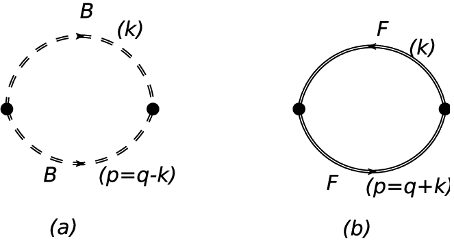
Now the Eq. (18) in static limit () gives a divergent value of . This can be easily seen when one uses the identity
| (19) |
so that Eq. (18) reduces to
| (20) | |||||
where with for and for is used which clearly diverges in the limit 0. However for interacting particles will be finite and the delta functions in Eq. (18) get replaced by a spectral function with a finite thermal width.
This adoption of finite thermal width is a very traditional technique in Kubo framework to get a non-divergent and finite value of transport coefficients. This is inversely related with relaxation time . The relevant vertex like factors are obtained as [79, 10, 73]
| (21) |
and using these in Eq. (20), we get expressions of different transport coefficients, as given in Eqs. (22), (23) and (24) respectively.
| (22) | |||||
| (23) |
| (24) |
where is degeneracy factor of medium constituents and is relaxation time. The degeneracy factor can in general we written as the product of degeneracies due to spin, color, number of flavors and particle and anti-particle. For example degeneracy for quark is 2(spin)(flavor)(quark and anti-quark)=8 and sum over the color is still to be taken.
Let us first note that the background gluon field couples to quarks through the covariant derivative as . In the Polyakov gauge, the Wilson line is in the diagonal representation in the color space and therefore, the background gluon field acts as an imaginary chemical potential for the colored particles. The corresponding color dependent equilibrium distribution function for the quarks and the anti-quarks are then given by [81]
| (25) |
where, we have written , without any summation over the index . As is traceless, . The Polyakov loop is thus related to as . Further, for vanishing baryon density, one can choose to be real and parameterize with as the dimensionless condensate variable. The Polyakov loop variable is therefore given by
| (26) |
It is easy to check that the the distribution function of Eq.(11) is the color averaged distribution function i.e. .
Let us note that in Eq.(20) the summation over all the colors for the fermion loops needs to be done. Thus while summing over colors one has
where, is the denominator of the Polyakov loop distribution function (11), . Let us note that one might further approximate the color dependent distribution functions by their color averaged distribution function of Eq.(11) in which case
| (28) |
In such cases e.g., the expression for becomes the more familiar expression as
| (29) |
One may note that such a replacement of color averaged distribution function is exact in the Boltzmann limit. Further difference between replacing the color distribution functions and their color averaged one is proportional to . This difference is small both below and above the critical temperature while it can be relevant around the critical temperature.
So far we have been concerned with the transport coefficients of quark components, where we have to take care of FD distribution with color degrees of freedom, which ultimately gives the Polyakov loop distribution function. However, for meson components, we have to use just BE distribution function in the of Eqs. (22), (23) and (24).

2.3 Thermal widths of quarks and mesons
We have calculated the thermal widths of different components from the imaginary part of their self energies. Unlike the vacuum case, for finite temperature, these thermal widths have contributions from both the decay processes and scattering processes involving particles present in the medium. Depending on the mass of the component we are interested in, either of the processes can become dominant. In our calculations, we found that for sigma meson, the mass is such that decay process dominates whereas, for pion and quark cases, the scattering is the dominant process. Thus to calculate the thermal width of quarks and mesons, we have to use relevant interaction part from the total Lagrangian density, addressed in Eq. (1). From Eq. (2), we can identify interaction Lagrangian density:
| (30) |
which will help us to calculate mesonic thermal widths . Similarly to calculate quark thermal widths , we need to identify the interaction part from Eq. (1). Expanding this interaction Lagrangian density and dividing it into and components, we get
| (31) |
and
| (32) |
respectively.
The quark thermal width, , can be estimated from the retarded part of the quark self-energy at finite temperature for quark-meson loops, where as shown in Fig 2(a). With the help of interaction Lagrangian densities (31) and (32), we obtain
| (33) | |||||
where and are the FD and BE distribution functions for intermediate and states respectively. Here, we can again replace by color average thermal distribution or Polyakov loop distribution . Now as mentioned earlier the relevant process for quark is the QQ or QQ scattering processes, analyzing the detailed branch cuts of this quark self-energy at finite temperature, one should notice that the quark pole () remains within the Landau-cut (cut corresponding to the scattering process) region( () of loop, when . Therefore, we will get non-zero values of only in the temperature region, where . This Landau cut contribution of quark self-energy basically interprets forward and backward quark-meson scattering, by which mesons are absorbed and emitted respectively [21].
Similarly, thermal widths of pion and sigma mesons and can be estimated from the retarded part of the meson self-energies and respectively, which are represented by Fig 2(b) in a general form. Using the interaction Lagrangian density (30), they are respectively derived as
and
where and are BE distribution functions for intermediate and states respectively.
Analyzing the detailed branch cuts of pion and sigma meson self-energies at finite temperature, one can find that the pion pole () and sigma pole () are respectively situated in the Landau-cut () and unitary-cut () regions for certain temperature range, where . Here, Landau cut contribution of pion self-energy measures the probabilities of forward and backward - scattering, where a is absorbed by former process and emitted by latter one. Next, the unitary cut contribution of meson self-energy signifies forward and backward decay processes - and respectively. Unlike the earlier Landau cuts for quark and pion self-energies, the unitary cuts of meson self-energy remains non-vanishing at as it is associated with forward decay process. At finite temperature, this unitary cut contribution gives a Bose-enhanced probability of this forward decay process and also an in-medium probability of backward decay process, which is absent in vacuum.
3 Numerical results and discussion

Let us start our numerical investigations by using the expressions of , and , given in Eqs. (2224). At first, instead of using explicit temperature () and momentum () dependent thermal width of quarks and mesons, constant values will be considered to highlight the thermodynamical phase space structure of different transport coefficients. This study is important as strong dependence of thermal width sometimes dominates over the dependence of phase-space part. For example, we have conformal symmetry breaking term in phase-space part of bulk viscosity expression (23), which generally gives a peak structure near the transition temperature. Hence, bulk viscosity able to map that peak structure only for a mild dependent or constant values of thermal width of medium constituents as we notice in Refs. [54, 45, 42, 43, 21]. However, a strong dependent thermal width or relaxation time can suppress the foot print of peak structure as observed in Refs. [22, 20, 19, 21].
The results of for constant , and are plotted by dashed, dotted and dash-dotted lines in Fig. 3(a). One can define their respective relaxation times , and using the relation and we have fixed their values to 1 fm as a typical value. The total shear viscosity is denoted by solid line in Fig. 3(a), which shows the dominant contribution of the quark component, compared to the contributions of the components and mesons. of all components and their total appear as increasing functions of but they exhibit some changes in their rate of increase near the transition temperature . Here, we assume that the interactions are well localized in space and time, so that total energy-momentum tensor, electromagnetic current for the multi-component system can be approximated as a sum of independent contributions [18]. Therefore, total transport coefficient is just considered as summation of individual components.
The Fig. 3(b) shows the variation for with temperature for respective components and their total, where we notice that mesonic components decrease and quark component increases with temperature. The increasing trend of total in the quark temperature domain is supported by the results of Ghosh et al. [21] (cyan triangles) and Marty et al. [20] (violet squares). The decreasing trend of the ratio below the transition temperature is also in agreement with the standard hadronic model calculations [8, 9, 10, 11, 12, 13, 14, 15, 16, 17]. Total is above the so-called KSS bound [75].
Following same notations of curves in Fig. (3), the temperature dependence of and are shown in Fig. 4(a) and (b) respectively. Here, we are observing a sharp peak structure in and near . The peak structures of pion and sigma components dominate compared to that of quark component. To understand this, we have to focus on the conformal symmetry breaking terms [18, 21] and in the integrand of Eq. (23), where is the temperature dependent mass of medium constituent. Near , the contribution of these quantities become maximum, which is at the root of this peak structure in . Hence, one can associate this peak structure of with the maximum violation of conformal symmetry breaking near . The first term of conformal symmetry breaking is same for all components, while second one is different for three different components. Rate of change of their masses with temperature reach their extrema near , which is responsible for making peaks in their ’s. Interestingly, sigma meson component shows two peak structure because of the non-monotonic changes of its mass with temperature. Such a peak structure has also been observed in the earlier calculations, based on Linear Sigma Model [18, 43] and Nambu-Jona-Lasinio model [21], where similar kind of peak structure in near were observed. We may assume indication of similar kind of peak structure from the increasing nature of [15, 17] in the hadronic temperature range and the decreasing nature of [41, 46, 47] in the temperature region of quark phase. Fig. 4(b) has included some earlier results of by Ghosh et al. [21] (triangles), Kadam et al. [15] (solid squares), Karsch et al. [47] (stars), Hostler et al. [17] (blue circles), Marty et al. [20] (open squares), whose order of magnitude is roughly close to the present estimations.
Next, Fig. 5(a) and (b) respectively show the electrical conductivity and the dimensionless quantity for different components of the medium. Using Eqs. (24) for different constituents, the results for quark (dashed line), pion (dotted line) components and their total (solid line) are calculated, where charge neutral constituents like and do not come into the picture. Similar to shear viscosity, of different components and their total are increasing functions of with some changes in their rate of increments near the transition temperature . The of quark component is much larger than that of pion component at high domain but in low temperature domain, pion component is dominant over quark component. In the hadronic temperature domain, of Refs. [68, 69, 67] are more or less in the same order of magnitude as our result. In this context, there are large numbers of works in LQCD approach with different numerical strengths of . Some of them [58, 59, 55] are displayed in Fig. 5(b) at certain (). A temperature dependent data (open circles) for is also added from the latest version of Ref. [57].

.


So far, the results of transport coefficients , and are obtained for constant thermal widths of medium constituents to highlight the phase-space structure of these coefficients. Now we proceed to estimate these transport coefficients for explicit and dependent thermal width. Before that, let us discuss in detail the structure of thermal widths for different medium constituents and then the results of different transport coefficients using those temperature and momentum dependent ’s. For quark thermal width , let us first concentrate on Eq. (33), which gives the on-shell value () of the imaginary part of quark self-energy for quark-meson loops. We can see the invariant mass distribution of by transforming the on-shell relation to the off-shell one in Eq. (33), where is invariant mass of quark. Now we can expect to observe a scattering (pion, quark) or decay (sigma) interaction at a particular temperature if the pole mass of the constituent lies within the range, where the invariant mass distribution of the thermal width is nonzero. For temperature GeV and quark momentum GeV, Fig. 6(a) shows the structure of (dashed line). Here the straight vertical blue line denotes the on-shell (constituent) quark mass at GeV, obtained within PQM model. We can see that the is away from the Landau cut region () of quark self-energy, where is non-zero. Therefore, the on-shell value of at GeV is zero, which we can see from the dashed line of Fig. 7(b). Remembering the discussion related to this issue after Eq. (33), we can get a non-zero on-shell value of beyond the Mott temperature , from where the threshold condition of interaction will be valid. In other words, we can say that will be within the Landau cut region of quark self-energy for .
Imposing similar kind of off-shell condition in Eqs. () and () for and mesons, one obtains and which are shown in Fig. 6(b) and (c) respectively. We see that the on-shell masses of and mesons at GeV, indicated by blue vertical lines in Fig. 6(b) and (c), are located within the respective branch cuts of their self-energies. Therefore, we will get non-zero on-shell values of and at GeV. After a certain temperature, from where the threshold condition of interaction is not valid, the on-shell values of and will vanish. This fact becomes more clear in Fig. 7(b), where on-shell values of (dotted line), (dash-dotted line) and (dashed line) are plotted against axis. Now following our previous discussion in section 2.3, we see that is only smaller than or for (Mott temperature) and it is never greater than the sum of the masses of any two components. So as we mentioned earlier it will only go through scattering processes and that is also only for a limited temperature region which we can clearly see in the lower panel, where remains zero in hadronic temperature region. Beyond the Mott temperature, it gets the non-zero value. Similarly we notice that and are non-zero in hadronic temperature range and beyond the Mott temperature, they vanish. These dependence of thermal widths are mainly controlled by the dependence of , and , which are shown by dashed, dotted and dash-dotted lines respectively in Fig. 7(a). The masses of and mesons are basically obtained from the Eqs. (7) and (9). In the chirally broken phase, the pion mass, being the mass of an approximate Goldstone mode, is protected and varies weakly with temperature. On the other hand, the mass of , which is approximately twice of the constituent quark mass, drops significantly near the transition temperature. At high temperature, being chiral partners, the masses of and mesons become degenerate and increase linearly with temperature. The temperature dependence of quark mass is mainly determined by the temperature dependence of chiral order parameter , which decreases with temperature to small values but never vanishes. On the other hand, the Polyakov loop parameter grows from to at high temperatures. This decreasing and increasing nature of and respectively signify the chiral and confinement properties of quark-hadron phase transition and are reflected in the temperature dependence of quark and meson masses. The transport coefficients thus depend both on the phase space factors and the momentum dependent widths.


Now, when we use the explicit structure of in Eqs. (33), () and (), the Figs. (3), (4) and (5) are respectively transformed to Figs. (8), (9) and (10), which have now additional influence of temperature dependent thermal widths along with the phase space part. We have split the temperature region into two parts because of the kinematic thresholds for mesons and quark self-energies. The first part, covering the hadronic temperature range, is for the results of pion component, while the results of quark component are plotted in the second part, which can be considered as quark temperature region. Since the results of meson component is negligible, because of its high values of as well as in the hadronic temperature range, the results of pion component only are shown in the panel of hadronic temperature region. Let us first come to the Fig. 8, where and for pion and quark components are described in panels (a), (b), (c) and (d) respectively. The blowing up tendency of for pion component in high domain is because of the suppressing tendency of , as shown previously by the dotted line in Fig. 7(b). Similarly, the result of for quark component is also limited within a particular (high) temperature domain because the non-zero structure of is limited within that -zone, as shown previously by the dashed line in Fig. 7(b). That is why we should focus on the order of magnitude for the transport coefficients instead of those blowing up regions. By using this kind of , not only but also other transport coefficients follow this pattern, which also observed in the earlier Ref. [21]. Fig. 8(b) shows that the for pion component from our calculation has, approximately, same order of magnitude as the results of Kadam et al. [16] (blue circles), Gorenstein et al. [14] (green squares). The corresponding results for quark component in its range agree with the earlier results obtained by Deb et al. [22] (green circles) and Marty et al. [20] (solid and open squares for two different models).
Following similar pattern of Fig. (8), Fig.9(a) to (d) show the and for pion and quark components, whose order of magnitude are comparable with results of Dobado et al. [43] (violet diamonds) in the hadronic temperature range and Arnold et al. [39, 1] (blue triangles) in the quark temperature domain. Next, using the same and dependent thermal widths, the electrical conductivity and for pion and quark components are plotted in Fig. (10). Numerical values of , obtained by us, are compared with the results of Marty et al. [20] (open squares), Cassing et al. [63] (blue pluses), Fraile et al. [69, 10] (magenta stars) in the hadronic temperature domain, whereas in the quark temperature domain, the values of our are compared with the results of Cassing et al. [63] (blue pluses) and Puglisi et al. [64] (open circles).
One may note that the present estimation of the transport coefficients in divided into two narrow temperature intervals about the Mott temperature. Below the Mott temperature, one has contributions from hadrons, namely pions and sigma while above the Mott temperature one has contributions from quarks. Below the Mott temperature the dominant contribution to transport coefficients comes from pions. The kinematic constriant of m translates into an upper cutoff on temperature for this process. Similary above the Mott temperature the constraint m imposes a lower cut off on temperature. As shown in Fig. 7.b., vanishes for large temperatures. Thus the 12 processes considered in this work results in the two narrow intervals near Mott temperature. However the temperature ranges of these intervals can be extended by including off shell contribution as has been considered in Ref [26]. Besides the calculation can be improved by including 22 scattering process which will not be restricted by such kinematic constriants [28].
One may observe from this investigation that near (but above) the Mott temperature scattering plays an important role as including these interactions result in a ratio of close to the conjectured KSS lower bound of . In the temperature interval above Mott temperature, the divergent nature of the transport coefficients at high temperatures reflect the fact that scattering contribution to vanishes. Although, one can expect an approximately constant values of ( if one considers the elastic scattering of quark-quark and quark-meson interaction as discussed in Ref. [28].
We might realize here that a small value of near the transition temperature is a reflection of an inherent non-perturbative feature captured by effective models like NJL [19, 20, 22] and PQM [28] models unlike pQCD calculations at high temperature [4]. Such models consider elastic scatterings. The inclusion of in-elastic scattering component with those earlier estimations will lead a further reduction of near the Mott temperature. Similar effects are also expected in other transport coefficients like bulk viscosity and electrical conductivity.
The present approximation of estimating the transport coefficients is similar to quasi-particle and relaxation time approximation of the boltzmann equation as done in Ref [18]. Within this approximation the contritbution of different species for transport coefficients are added. Whereas to calculate the relaxation time for given species the relaxation times of scattering and decay involving other particles are added inversely. Therefore the effect of interactions with other species is also included in the evaluation of relaxation time and hence on the transport coefficient.
4 Summary and Perspectives
In this article, we have investigated the role of PQM dynamics in calculations of different transport coefficients like shear viscosity , bulk viscosity and electrical conductivity of quark and hadronic medium with zero quark chemical potential. We have first briefly sketched the background framework of Kubo method to obtain the standard expressions of , and . We have also shown explicitly how the polyakov loop affects the thermal distribution functions of quarks which appear in calculation of transport coefficients.
The temperature dependence of transport coefficients depends on two parts - one is thermodynamical phase-space structure and other is thermal width of respective transport correlators. To distinguish between the two effects, we have taken constant thermal width for different transport correlators, which essentially reveals the effect of the phase-space structure on different transport coefficients. The phase-space structure of transport coefficients is mostly governed by the temperature dependent masses of the quark and mesons in PQM model. The temperature dependence of the masses is governed by the chiral symmetry restoration in the model at high temperature. and show an increasing behavior with temperature without much sigmnificant changes at the quark-hadron transition temperature.
Interestingly, even with constant decay width shows a minimum at the tranisition temperature.
On the other hand exhibits a peak structure near the transition temperature. Unlike and , the expression of additionally contains conformal breaking terms of QCD medium apart from phase space structure, whose peak pattern is reflected in temperature dependence of . The qualitative profiles of , and vs are in agreement with the earlier studies, based on different dynamical models.
Next, we have considered the explicit temperature and momentum dependence of for quark and mesons to estimate the values of those transport coefficients. In our earlier work [28], the quark and pion thermal widths or their inverse (relaxation times) have been calculated using kind of elastic channels, for which we get near the Mott temperature. In present work, we have focussed on kind of in-elastic channels of quarks and mesons, which are calculated from the imaginary part of their self-energies at finite temperature. For quark self-energy, quark-pion and quark-sigma meson loops are taken while pion-sigma and pion-pion loops are taken to obtain pion and sigma meson self-energies respectively. The thermal widths of quark and mesons are found to be non-zero in limited regions of high and low temperature domain because of their respective threshold conditions. Therefore, when we estimate different transport coefficients using those thermal widths, we are able to predict their values within those temperature ranges only. Interestingly, we notice that near (but above) the Mott temperature, can reach the KSS value () because of such inelastic scattering processes. The contribution of inelastic channels to the calculation of thermal widths may be comparable, or may even be dominant, to those of elastic scatterings,. Although beyond a certain temperature, the contribution of in-elastic scattering vanishes and only elastic channels [28] survive leding to low .
The present work of two flavor PQM model can be generalized to a more realistic 2 +1 flavor model. With more number of mesons there are many more channels involving the strange quarks. It will be interesting to look at the different branch cut structure due to the difference in masses of the strange and non strange quarks. Calculations in this regard are in progress and will be reported in future.
Acknowledgment: PS is supported from the scheme of DST Inspire (India). SG acknowledges to IIT-Bhilai, funded by Ministry of Human Resource Development (MHRD), Govt. of India. SG would like to thank to Sandeep Chatterjee, Bhaswar Chatterjee, Snigdha Ghosh and Purushottam Sahu for getting some help on this work. Authors are very thankful to Kinkar Saha and Rajarshi Ray for their useful comments. SG, AA and HM acknowledge WHEPP-2017 for getting some fruitful discussions. GK is financially supported by the DST-INSPIRE faculty award under Grant No. DST/INSPIRE/04/2017/002293.
References:
References
- [1] J. I. Kapusta, Relativistic Nuclear Collisions, Landolt-Bornstein New Series, Vol. I/23, ed. R. Stock (Springer-Verlag, Berlin Heidelberg 2010).
- [2] P. Romatschke and U. Romatschke, Phys. Rev. Lett. 99, 172301 (2007); T. Hirano and M. Gyulassy, Nucl. Phys. A769, 71 (2006).
- [3] C. Gale, S. Jeon, and B. Schenke, Int. J. Mod. Phys. A28, 134011 (2013).
- [4] P. B. Arnold, G. D. Moore, and L. G. Yaffe, J. High Energy Phys. 11 (2000) 001; 05 (2003) 051.
- [5] N. Christiansen, M. Haas, J. M. Pawlowski, N. Strodthoff, Phys. Rev. Lett. 115, 112002 (2015).
- [6] H. B. Meyer, Phys. Rev. D 76, 101701 (2007); Phys. Rev. D 82, 054504 (2010).
- [7] N. Astrakhantsev, V. Braguta, A. Kotov, J. High Energy Phys. 1704 (2017) 101; J. High Energy Phys. 1509 (2015) 082.
- [8] K. Itakura, O. Morimatsu, and H. Otomo, Phys. Rev. D 77, 014014 (2008).
- [9] A. Dobado and S.N. Santalla, Phys. Rev. D 65, 096011 (2002); A. Dobado and F. J. Llanes-Estrada, Phys. Rev. D 69, 116004 (2004).
- [10] D. Fernandez-Fraile and A. Gomez Nicola, Eur. Phys. J. C 62, 37 (2009).
- [11] R. Lang, N. Kaiser and W. Weise Eur. Phys. J. A 48, 109 (2012).
- [12] S. Mitra, S. Ghosh, and S. Sarkar Phys. Rev. C 85, 064917 (2012).
- [13] S. Ghosh, G. Krein, S. Sarkar, Phys. Rev. C 89, 045201 (2014); S. Ghosh, Phys. Rev. C 90 025202 (2014); S. Ghosh, Braz. J. Phys. 45 (2015) 687.
- [14] M. I. Gorenstein, M. Hauer, O. N. Moroz, Phys. Rev. C 77, 024911 (2008).
- [15] G. P. Kadam and H. Mishra, Nucl. Phys. A 934, 133 (2015).
- [16] G. P. Kadam and H. Mishra, Phys. Rev. C 92, 035203 (2015).
- [17] J. Noronha-Hostler, J. Noronha, C. Greiner, Phys. Rev. Lett. 103, 172302 (2009).
- [18] P. Chakraborty and J. I. Kapusta, Phys. Rev. C 83, 014906 (2011).
- [19] C. Sasaki, K. Redlich, Nucl. Phys. A 832 (2010) 62.
- [20] R. Marty, E. Bratkovskaya, W. Cassing, J. Aichelin, H. Berrehrah, Phys. Rev. C 88 (2013) 045204.
- [21] S. Ghosh, T. C. Peixoto, V. Roy, F. E. Serna, and G. Krein, Phys. Rev. C 93, 045205 (2016).
- [22] P. Deb, G. Kadam, H. Mishra, Phys. Rev. D 94 (2016), 094002.
- [23] A. N. Tawfik, A. M. Diab, M.T. Hussein, Int.J.Mod.Phys. A31 (2016) 1650175; arXiv:1610.06041 [nucl-th].
- [24] S. Ghosh, A. Lahiri, S. Majumder, R. Ray, S. K. Ghosh, Phys. Rev. C 88 (2013) 068201.
- [25] R. Lang, W. Weise Eur. Phys. J. A 50, 63 (2014).
- [26] R. Lang, N. Kaiser, W. Weise, Eur. Phys. J. A 51, 127 (2015).
- [27] A. Harutyunyan, D. H. Rischke, A. Sedrakian, Phys.Rev. D 95 (2017) 114021.
- [28] A. Abhishek, H. Mishra, S. Ghosh, Phys. Rev. D 97 (2018) 014005.
- [29] S. K. Ghosh, S. Raha, R. Ray, K. Saha, S. Upadhaya, Phys. Rev. D 91, 054005 (2015).
- [30] N. Demir and S.A. Bass Phys. Rev. Lett. 102, 172302 (2009).
- [31] A. Muronga, Phys. Rev. C 69, 044901 (2004).
- [32] S. Plumari, A. Puglisi, F. Scardina, and V. Greco, Phys. Rev. C 86, 054902 (2012).
- [33] S. Pal, Phys. Lett. B 684 (2010) 211.
- [34] N. Sadooghi, F. Taghinavaz, Phys. Rev. D 89, 125005 (2014).
- [35] M. Albright and J. I. Kapusta, Phys. Rev. C 93, 014903 (2016).
- [36] M. Prakash, M. Prakash, R. Venugopalan, and G. Welke, Phys. Rep. 227, 321 (1993).
- [37] S. Gavin, Nucl. Phys. A, 435, 826 (1985).
- [38] K. Paech and S. Pratt, Phys. Rev. C 74, 014901 (2006).
- [39] P. Arnold, C. Dogan, G. D. Moore, Phys. Rev. D 74, 085021 (2006).
- [40] S. K. Das, J. Alam Phys.Rev. D 83 (2011) 114011.
- [41] H. B. Meyer, Phys. Rev. Lett. 100, (2008) 162001.
- [42] A. Dobado, F.J.Llane-Estrada, J. Torres Rincon, Phys. Lett. B 702, 43 (2011).
- [43] A. Dobado, J. Torres Rincon, Phys. Rev. D 86, 074021 (2012).
- [44] C. Sasaki, K. Redlich, Phys. Rev. C 79, 055207 (2009).
- [45] X. Shi-Song, G. Pan-Pan, Z. Le, H. De-Fu, Chin. Phys. C 38, (2014) 054101.
- [46] D. Kharzeev, K. Tuchin, JHEP 0809, 093 (2008).
- [47] F. Karsch, D. Kharzeev, K. Tuchin, Phys. Lett. B 663 (2008) 217.
- [48] V. Chandra, Phys. Rev. D 86 (2012) 114008; Phys. Rev. D 84 (2011) 094025.
- [49] D. Fernandez-Fraile and A. Gomez Nicola, Phys. Rev. Lett. 102, 121601 (2009).
- [50] S. Mitra and S. Sarkar, Phys. Rev. D 87, 094026 (2013); S. Mitra, S. Gangopadhyaya, and S. Sarkar, Phys. Rev. D 91, 094012 (2015).
- [51] S. Ghosh, S. Chatterjee, B. Mohanty Phys. Rev. C 94 (2016) 045208.
- [52] G. Sarwar, S. Chatterjee, Jane Alam arXiv: 1512.06496[nucl-th].
- [53] G. P. Kadam, H. Mishra, Phys.Rev. C 93 (2016) 025205.
- [54] K. Saha, S. Upadhaya, S. Ghosh, Mod. Phys. Lett. A 32 (2016) no.05, 1750018.
- [55] H.T. Ding, A. Francis, O. Kaczmarek, F. Karsch, E. Laermann, and W. Soeldner, Phys. Rev. D 83, 034504 (2011).
- [56] G. Aarts, C. Allton, A. Amato, P. Giudice, S. Hands and J. Skullerud, J. High Energy Phys. 02 (2015) 186;
- [57] G. Aarts, C. Allton, J. Foley, S. Hands, and S. Kim, Phys. Rev. Lett. 99, 022002 (2007).
- [58] P. V. Buividovich, M. N. Chernodub, D. E. Kharzeev, T. Kalaydzhyan, E. V. Luschevskaya, and M. I. Polikarpov, Phys. Rev. Lett. 105, 132001 (2010).
- [59] Y. Burnier and M. Laine, Eur. Phys. J. C 72, 1902 (2012).
- [60] S. Gupta, Phys. Lett. B 597, 57 (2004).
- [61] B. B. Brandt, A. Francis, H. B. Meyer, and H. Wittig, J. High Energy Phys. 03 (2013) 100.
- [62] A. Amato, G. Aarts, C. Allton, P. Giudice, S. Hands, J.I. Skullerud, Phys. Rev. Lett. 111, 172001 (2013).
- [63] W. Cassing, O. Linnyk, T. Steinert, and V. Ozvenchuk, Phys. Rev. Lett. 110, 182301 (2013).
- [64] A. Puglisi, S. Plumari, V. Greco, Phys. Rev. D 90, 114009 (2014); J. Phys. Conf. Ser. 612 (2015) 012057; Phys. Lett. B 751 (2015) 326.
- [65] M. Greif, I. Bouras, Z. Xu, C. Greiner, Phys. Rev. D 90 (2014) 094014; J. Phys. Conf. Ser. 612 (2015) 012056.
- [66] P. K. Srivastava, L. Thakur, B. K. Patra, Phys. Rev. C 91, 044903 (2015).
- [67] S. I. Finazzo, J. Noronha Phys. Rev. D 89, 106008 (2014).
- [68] C. Lee, I. Zahed, Phys. Rev. C 90, 025204 (2014).
- [69] D. Fernandez-Fraile and A. Gomez Nicola, Phys. Rev. D 73, 045025 (2006).
- [70] M. Greif, C. Greiner, G.S. Denicol, Phys. Rev. D 93, 096012 (2016).
- [71] S. Ghosh, F. E. Serna, A. Abhishek, G. Krein, H. Mishra, arXiv:1809.07594 [nucl-th]
- [72] S. Mitra and V. Chandra, Phys. Rev. D 94, 034025 (2016).
- [73] S. Ghosh, Phys. Rev. D 95 (2017) 036018.
- [74] B.-J. Schaefer, J. M. Pawlowski, J. Wambach, Phys. Rev. D 76, 074023 (2007).
- [75] P. Kovtun, D. T. Son, and O. A. Starinets, Phys. Rev. Lett. 94, 111601 (2005).
- [76] D. N. Zubarev Non-equilibrium statistical thermodynamics (New York, Consultants Bureau, 1974).
- [77] R. Kubo, J. Phys. Soc. Jpn. 12, 570 (1957).
- [78] M. S. Green, J. Chem. Phys. 22, 398 (1954).
- [79] S. Ghosh, Int. J. Mod. Phys. A 29 (2014) 1450054.
- [80] S. Jeon, Phys. Rev. D 52 (1995) 3591.
- [81] Y. Hidaka, S. Lin, R. D. Pisarski and D. Satow, J. High Energy Phys. 10,005, (2015).
- [82] A. Abhishek, H. Mishra, S. Ghosh, PoS CPOD2017 (2018) 080, arXiv:1801.04393 [hep-ph].
- [83] G.S. Denicol, C. Gale, S. Jeon and J. Noronha Phys. Rev. C 88(2013) 064901
- [84] C.R. Wilke, J. Chem. Phys. 18, 517 (1950).
- [85] S. Mathur, S.C. Saxena, Applied Scientific Research, Section A, 15, 203 (1966).