Floquet multi-Weyl points in crossing-nodal-line semimetals
Abstract
Weyl points with monopole charge have been extensively studied, however, real materials of multi-Weyl points, whose monopole charges are higher than , have yet to be found. In this Rapid Communication, we show that nodal-line semimetals with nontrivial line connectivity provide natural platforms for realizing Floquet multi-Weyl points. In particular, we show that driving crossing nodal lines by circularly polarized light generates double-Weyl points. Furthermore, we show that monopole combination and annihilation can be observed in crossing-nodal-line semimetals and nodal-chain semimetals. These proposals can be experimentally verified in pump-probe angle-resolved photoemission spectroscopy.
Stimulated by extensive studies on topological insulators [1, 2, 3], it has now been realized that many metals also have topological characterizations[3, 4, 5]. In these topological semimetals, the valence band and conduction band touch at certain -space manifolds. When the band-touching manifolds consist of isolated points, the materials are nodal-point semimetals, Dirac semimetals[6, 7, 8, 9, 10, 11, 12, 13, 14, 15] and Weyl semimetals(WSMs)[16, 17, 18, 19, 20, 21, 22, 23, 24, 25, 26, 27, 28, 29, 30, 31, 32, 33, 34, 35, 36, 37, 38, 39] being the most well-known examples; when the band-touching manifolds are one-dimensional lines, the systems are nodal-line semimetals(NLSMs)[40, 41, 42, 43, 44, 45, 46, 47, 48, 49, 50, 51, 52, 53, 54, 55, 56, 57, 58, 59, 60, 61, 62, 63, 64, 65, 66, 67, 68, 69, 70, 71, 72, 73, 74, 75, 76, 77].
In WSMs, the Weyl points are the sources or sinks of Berry magnetic field, namely, they are the Berry monopole charges. The total number of monopole charge in the Brillouin zone must be zero, which has been formulated decades ago as a no-go theorem by Nielsen and Ninomiya[78]. Usually, a Weyl point has a linear dispersion in all three spatial directions, with a low-energy Hamiltonian , where are the Pauli matrices. The monopole charge is just . Interestingly, multi-Weyl points with monopole charge higher than one are also possible. The simplest cases are the double-Weyl points with [79, 80, 81], which have novel physical consequences[82, 83, 84, 85, 86, 87]. So far, the double-Weyl points have not been experimentally realized in solid-state materials. Considering the widespread interests in WSMs, it is highly interesting to find material realizations of multi-Weyl points. The combination of several Weyl points into a multi-Weyl point, and the annihilation of several Weyl points are even more interesting to investigate, nevertheless, it is challenging to do so because of the limited tunability in the samples.
Over the past few years, periodic driving has been used as a powerful method to alter the topology of static systems, and more remarkably, to create new topological phases without analog in static systems[88, 89, 90, 91, 92, 93, 94, 95, 96, 97, 98, 99, 100, 101, 102, 103, 104, 105, 106, 107, 108, 109]. Recently, there are a few theoretical proposals for Floquet topological semimetals[110, 111, 112, 113, 114, 115, 116, 117, 118, 119, 120, 121], in particular, it has been suggested that under a circularly polarized light (CPL), NLSMs will be driven to Floquet WSMs with highly tunable Weyl points [116, 117, 118, 122]. In these studies, only the simplest nodal lines are considered. The present work is stimulated by recent proposals of novel nodal lines with nontrivial connectivity, including crossing nodal lines[54, 55, 123, 124] (probably the most interesting ones are the nodal chains[58, 125, 126]), nodal links[127, 128, 129, 130], and nodal knots[131]. In this Rapid Communication, we show that crossing nodal lines (including nodal chains) are natural platforms for the realizations of Floquet multi-Weyl points and the combinations (annihilations) of Weyl points. In particular, a two-nodal-line crossing point can be driven to a double-Weyl point, and tuning the direction of incident lasers can induce monopole combination transitions. Considering the abundant material candidates for crossing nodal lines[52, 53, 54, 55, 123, 56, 57, 58], we believe that this proposal can be experimentally verified in the near future.
Double-Weyl points from Type-I crossing.— For simplicity, we focus on NLSMs with negligible spin-orbit coupling[54, 55]. We distinguish two types of nodal line crossing, illustrated in Fig.1(a) and (b), as type-I and type-II crossing, respectively. The type-II crossing is the basic building block of nodal chains. In this section, we focus on the type-I crossing. Our starting point is the following Bloch Hamiltonian ()
| (1) |
where are Pauli matrices in orbital space and is the identity matrix, is a positive constant with the dimension of energy, and are positive constants with the dimension of inverse energy, and . As the diagonal term does not affect the main physics, we will neglect it hereafter. The energy spectra of this Hamiltonian read
| (2) |
It is readily found that there are two nodal lines, one is located in the plane and determined by the equation , while the other one is located in the plane and determined by the equation . The two nodal lines cross at , which gives the type-I crossing illustrated in Fig.1(a). The crossing points are protected by the mirror symmetry: and with .


We study the effects of a CPL. Let us consider a CPL incident in the direction , where and is the polar and azimuthal angle in the spherical coordinate system, respectively. The vector potential of the light is , with corresponding to the right-handed and left-handed CPL, respectively. Here, and are two unit vectors perpendicular to , satisfying .
Following the standard approach, the electromagnetic coupling is given by . Since the full Hamiltonian is time-periodic, it can be expanded as with
| (3) |
and for ; , , . We focus on the off-resonance regimes, and the system is well described by an effective time-independent Hamiltonian, which reads[89, 132]
| (4) | |||||
where . Consequently, the energy spectra of are
| (5) | |||||
For a general incident direction other than , , and , , , it is readily found from Eq.(5) that there are four Floquet Weyl points. Since under experimental conditions, the term can be neglected because it only induces a small and trivial change to the positions of the Weyl points. Discarding the term, it is straightforward to determine the positions of the Weyl points, which are at
| (6) |
We can expand around these points as with referring to the momentum relative to the gapless points. The monopole charge of the Weyl point at is simply . A straightforward calculation gives
| (7) |
The number of monopole is equal to the number of antimonopole, automatically satisfying Nielsen-Ninomiya theorem[78]. From Eq.(6) and Eq.(7), it is readily seen that with the variation of and the handness of the light, both the positions and the monopole charges are tunable. Most interestingly, when the direction or is reached, we can observe the combination of two Weyl points with the same monopole charge to form a double-Weyl point. To see this more clearly, notice that when the light comes in the direction, i.e., , , in Eq.(4) reduces to the form of
| (8) |
which gives two gapless points at . A calculation of the Berry-flux number passing through the surface enclosing or yields the monopole charges, which are
| (9) |
i.e., they are double-Weyl points. A picture illustration of the motion and combination of Weyl points, as is tuned, is shown in Fig.2(a).
Before closing this section, we briefly discuss crossing nodal lines with cubic symmetry, keeping in mind that several material candidates of NLSM are found to belong to this class [55, 123, 56]. The cubic symmetry guarantees the existence of three nodal lines located in mutually orthogonal planes, and the nodal lines are mutually crossing. Since the crossing is still the type I, the physics of Floquet double-Weyl points and monopole combination is similar as that of Eq.(1) (see Supplemental Material for details).
Monopole annihilation from type-II crossing.— Now we turn to the type-II crossing [see Fig.1(b)], which serves as the key building block of nodal chain[58, 125, 126]. The local Hamiltonian near the type-II crossing point can be captured by the following continuum Hamiltonian
| (10) |
whose energy spectra are
| (11) |
Thus, there is a nodal ring at , , as well as two open nodal lines of hyperbolic shape at , . The three nodal lines touch at two points , which gives the type-II crossing shown in Fig.1(b).
Again we consider an incident light described by and follow the procedures of the previous section, we find that the effective Floquet Hamiltonian takes the form of[133]
| (12) | |||||
where , and . The term is fourth order in , which is small, thus we first neglect it.


For a general incident angle, similar to the type-I case, the effect of term can be neglected. It is straightforward to find the four Weyl points at
| (13) |
The corresponding monopole charges are found to be
| (14) |
Thus, both the positions and the monopole charges of the Weyl points are highly tunable. When the incident direction of the light is tuned to the direction, i.e., and , it is readily seen from Eq.(13) that and will overlap, similarly for and . Eq.(14) tells us that their monopole charges are opposite, thus, the annihilation of two Weyl points with opposite monopole charge will occur, and a gapless point with is found as the remnant of annihilation. To be explicit, let us write down for and :
| (15) |
There are only two gapless points, namely . It is readily found that the monopole charges of are both zero. In fact, the sign of the coefficient of is the same for all , preventing a nonzero winding of the pseudospin vector around the origin, thus the monopole charge has to vanish.
Thus, monopole annihilation can be observed using nodal lines with type-II crossing (Fig.2(b)). Since have vanishing monopole charge, they are unstable, i.e., they can be gapped out by a perturbation of the form ( denotes a constant).
Now we come back to the effects of the term. With the term, we find that the energy spectra have a small gap at when the light comes in the direction (i.e., a Floquet insulator). Therefore, when the direction of light is tuned away from the direction to other directions, the system undergoes an insulator-WSM transition at certain incident angle, namely, pairs of Weyl points with opposite monopole charges are created from the Floquet insulators.
Surface state evolution.— A key character of Weyl semimetals is the surface Fermi arcs. With the creation of multi-Weyl points, multiple Fermi arcs are naturally expected. We now check it by explicit calculations. Let us focus on the type-I crossing (the similar analysis of type-II crossing is given in Supplemental Material). We consider that the system occupies the region. The energy dispersion and the wave functions of the surface states can be determined by solving the eigenvalue problem , under the boundary conditions and . For simplicity, we neglect the term at this stage, and take the driving-induced term as a perturbation (this is justified as both and are small), namely, with
| (16) |
We first solve the eigenfunction , which gives and
| (17) |
with a normalization constant, and
| (18) |
The surface state exists only when , i.e., .

Now we add the perturbation , which modifies the dispersion as
| (19) | |||||
Consequently, the surface states of the driven system become dispersive and the dispersion is given by in this perturbation theory. For the double-Weyl point case, i.e., and , the energy dispersion reads
| (20) |
The surface state dispersions of the pristine crossing-nodal-line semimetal and the Floquet double-Weyl semimetal are shown in Fig.3. It is readily seen that the driving tears and tilts the flat drumhead surface band of the pristine NLSM, giving rise to two Fermi arcs. The number of Fermi arcs is equal to the monopole charge of the Weyl points.
Effect of spin-orbit coupling.— Now we discuss the effect of spin-orbit coupling (SOC). As long as the pristine crossing structure is robust against SOC, such as that of the proposed material IrF4[58], where it is protected by nonsymmorphic symmetries, the introduction of SOC will only induce a change in the positions of the Flqouet Weyl points. On the other hand, if the pristine crossing structure is fragile to SOC, such as that of the candidate CaTe, where the nodal lines are predicated to evolve into Dirac points in the presence of SOC[123], we find the Floquet double-Weyl points become unstable and will be split into Floquet single-Weyl points (Supplemental Material).
Experimental estimations.—Among other approaches, an optimal experimental method to verify this proposal is the pump-probe angle-resolved photoemission spectroscopy (ARPES)[102, 104, 105], which can directly measure the locations of double-Weyl points. Another approach is to measure the incident-angle-dependent Hall voltage, which is determined by the locations of the Floquet Weyl points[115, 116]. Here we provide an estimation based on the material candidate Cu3NPd[54, 55]. Under the experimental condition of ref.[102], is estimated to be of the order of , and a film sample with size mmnm can generate an incident-angle-dependent Hall voltage of the order of mV if a dc current of mA is applied in direction (Supplemental material), well within the capacity of current experiments.
Conclusions.—There have been extensive theoretical and experimental studies of Weyl points with monopole charge , however, multi-Weyl semimetals have not been well studied so far due to the lack of materials. Here, we show that multi-Weyl points can be realized in driven nodal-line semimetals with novel line-connectivity (crossing nodal lines and nodal chains). In addition to suggesting a way to realize multi-Weyl semimetals, this work indicates that novel nodal lines are versatile platforms in the field of topological semimetals. Our proposal may also be generalized to cold-atom systems where periodic driving can be realized by shaking the optical lattice[134, 135, 136].
Note added: Upon finishing this manuscript, we become aware of a related preprint[137], in which type-I crossing is studied.
Acknowledgements.— We would like to thank Gang Chen and Ling Lu for useful discussions. This work is supported by NSFC (No. 11674189). Z. Y. is supported in part by China Postdoctoral Science Foundation (No. 2016M590082).
References
- [1] M. Z. Hasan and C. L. Kane, Rev. Mod. Phys. 82, 3045 (2010).
- [2] X.-L. Qi and S.-C. Zhang, Rev. Mod. Phys. 83, 1057 (2011).
- [3] C.-K. Chiu, J. C. Y. Teo, A. P. Schnyder, and S. Ryu, Rev. Mod. Phys. 88, 035005 (2016).
- [4] N. P. Armitage, E. J. Mele, and A. Vishwanath, ArXiv e-prints (2017), arXiv:1705.01111 [cond-mat.str-el] .
- [5] Y. X. Zhao and Z. D. Wang, Phys. Rev. Lett. 110, 240404 (2013).
- [6] Z. Liu, B. Zhou, Y. Zhang, Z. Wang, H. Weng, D. Prabhakaran, S.-K. Mo, Z. Shen, Z. Fang, X. Dai, et al., Science 343, 864 (2014).
- [7] M. Neupane, S.-Y. Xu, R. Sankar, N. Alidoust, G. Bian, C. Liu, I. Belopolski, T.-R. Chang, H.-T. Jeng, H. Lin, A. Bansil, F. Chou, and M. Z. Hasan, Nature Communications 5, 3786 (2014), arXiv:1309.7892 [cond-mat.mes-hall] .
- [8] S. Borisenko, Q. Gibson, D. Evtushinsky, V. Zabolotnyy, B. Büchner, and R. J. Cava, Phys. Rev. Lett. 113, 027603 (2014).
- [9] S.-Y. Xu, C. Liu, S. K. Kushwaha, R. Sankar, J. W. Krizan, I. Belopolski, M. Neupane, G. Bian, N. Alidoust, T.-R. Chang, et al., Science 347, 294 (2015a).
- [10] Z. Wang, Y. Sun, X.-Q. Chen, C. Franchini, G. Xu, H. Weng, X. Dai, and Z. Fang, Physical Review B 85, 195320 (2012).
- [11] S. M. Young, S. Zaheer, J. C. Teo, C. L. Kane, E. J. Mele, and A. M. Rappe, Physical review letters 108, 140405 (2012).
- [12] Z. Wang, H. Weng, Q. Wu, X. Dai, and Z. Fang, Physical Review B 88, 125427 (2013a).
- [13] A. Sekine and K. Nomura, Phys. Rev. B 90, 075137 (2014).
- [14] C. Zhang, E. Zhang, Y. Liu, Z.-G. Chen, S. Liang, J. Cao, X. Yuan, L. Tang, Q. Li, T. Gu, Y. Wu, J. Zou, and F. Xiu, ArXiv e-prints (2015), arXiv:1504.07698 [cond-mat.mtrl-sci] .
- [15] B.-J. Yang and N. Nagaosa, Nature Communications 5, 4898 (2014).
- [16] X. Wan, A. M. Turner, A. Vishwanath, and S. Y. Savrasov, Phys. Rev. B 83, 205101 (2011).
- [17] S. Murakami, New Journal of Physics 9, 356 (2007).
- [18] H. B. Nielsen and M. Ninomiya, Physics Letters B 130, 389 (1983).
- [19] G. E. Volovik, The Universe in a Helium Droplet (Oxford University Press,USA, 2003).
- [20] K.-Y. Yang, Y.-M. Lu, and Y. Ran, Phys. Rev. B 84, 075129 (2011).
- [21] A. A. Burkov and L. Balents, Phys. Rev. Lett. 107, 127205 (2011).
- [22] D. T. Son and B. Z. Spivak, Phys. Rev. B 88, 104412 (2013).
- [23] Z. Wang and S.-C. Zhang, Phys. Rev. B 87, 161107 (2013).
- [24] L. Lu, L. Fu, J. D. Joannopoulos, and M. Soljačić, Nature photonics 7, 294 (2013).
- [25] P. Hosur and X. Qi, Comptes Rendus Physique 14, 857 (2013), arXiv:1309.4464 [cond-mat.str-el] .
- [26] L. Lu, J. D. Joannopoulos, and M. Soljacic, Nat Photon 8, 821 (2014).
- [27] H. Weng, C. Fang, Z. Fang, B. A. Bernevig, and X. Dai, Phys. Rev. X 5, 011029 (2015a).
- [28] S.-M. Huang, S.-Y. Xu, I. Belopolski, C.-C. Lee, G. Chang, B. Wang, N. Alidoust, G. Bian, M. Neupane, A. Bansil, H. Lin, and M. Zahid Hasan, Nature Communications 6, 7373 (2015).
- [29] S.-Y. Xu, I. Belopolski, N. Alidoust, M. Neupane, G. Bian, C. Zhang, R. Sankar, G. Chang, Z. Yuan, C.-C. Lee, S.-M. Huang, H. Zheng, J. Ma, D. S. Sanchez, B. Wang, A. Bansil, F. Chou, P. P. Shibayev, H. Lin, S. Jia, and M. Z. Hasan, Science 349, 613 (2015b).
- [30] B. Lv, H. Weng, B. Fu, X. Wang, H. Miao, J. Ma, P. Richard, X. Huang, L. Zhao, G. Chen, et al., Physical Review X 5, 031013 (2015).
- [31] X. Huang, L. Zhao, Y. Long, P. Wang, D. Chen, Z. Yang, H. Liang, M. Xue, H. Weng, Z. Fang, X. Dai, and G. Chen, Phys. Rev. X 5, 031023 (2015).
- [32] N. Ghimire, Y. Luo, M. Neupane, D. Williams, E. Bauer, and F. Ronning, Journal of Physics: Condensed Matter 27, 152201 (2015).
- [33] C. Shekhar, A. K. Nayak, Y. Sun, M. Schmidt, M. Nicklas, I. Leermakers, U. Zeitler, Y. Skourski, J. Wosnitza, Z. Liu, et al., Nature Physics 11, 645 (2015).
- [34] S.-Y. Xu, N. Alidoust, I. Belopolski, Z. Yuan, G. Bian, T.-R. Chang, H. Zheng, V. N. Strocov, D. S. Sanchez, G. Chang, et al., Nature Physics 11, 748 (2015c).
- [35] L. Lu, Z. Wang, D. Ye, L. Ran, L. Fu, J. D. Joannopoulos, and M. Soljačić, Science 349, 622 (2015).
- [36] J. Zhou, H.-R. Chang, and D. Xiao, Phys. Rev. B 91, 035114 (2015).
- [37] R. Bi and Z. Wang, Phys. Rev. B 92, 241109 (2015).
- [38] H.-Z. Lu and S.-Q. Shen, Frontiers of Physics 12, 127201 (2016).
- [39] B. Yan and C. Felser, Annual Review of Condensed Matter Physics 8, 337 (2017).
- [40] A. A. Burkov, M. D. Hook, and L. Balents, Phys. Rev. B 84, 235126 (2011).
- [41] J.-M. Carter, V. V. Shankar, M. A. Zeb, and H.-Y. Kee, Phys. Rev. B 85, 115105 (2012).
- [42] M. Phillips and V. Aji, Phys. Rev. B 90, 115111 (2014).
- [43] Y. Chen, Y.-M. Lu, and H.-Y. Kee, Nature communications 6, 6593 (2015a).
- [44] C.-K. Chiu and A. P. Schnyder, Phys. Rev. B 90, 205136 (2014).
- [45] K. Mullen, B. Uchoa, and D. T. Glatzhofer, Phys. Rev. Lett. 115, 026403 (2015).
- [46] G. Bian, T.-R. Chang, R. Sankar, S.-Y. Xu, H. Zheng, T. Neupert, C.-K. Chiu, S.-M. Huang, G. Chang, I. Belopolski, D. S. Sanchez, M. Neupane, N. Alidoust, C. Liu, B. Wang, C.-C. Lee, H.-T. Jeng, A. Bansil, F. Chou, H. Lin, and M. Zahid Hasan, Nature Communications 7, 10556 (2016).
- [47] L. S. Xie, L. M. Schoop, E. M. Seibel, Q. D. Gibson, W. Xie, and R. J. Cava, APL Mater. 3, 083602 (2015).
- [48] Y. Chen, Y. Xie, S. A. Yang, H. Pan, F. Zhang, M. L. Cohen, and S. Zhang, Nano Letters 15, 6974 (2015b).
- [49] C. Fang, Y. Chen, H.-Y. Kee, and L. Fu, Phys. Rev. B 92, 081201 (2015).
- [50] G. Bian, T.-R. Chang, H. Zheng, S. Velury, S.-Y. Xu, T. Neupert, C.-K. Chiu, S.-M. Huang, D. S. Sanchez, I. Belopolski, N. Alidoust, P.-J. Chen, G. Chang, A. Bansil, H.-T. Jeng, H. Lin, and M. Z. Hasan, Phys. Rev. B 93, 121113 (2016).
- [51] Y.-H. Chan, C.-K. Chiu, M. Y. Chou, and A. P. Schnyder, Phys. Rev. B 93, 205132 (2016a).
- [52] M. Zeng, C. Fang, G. Chang, Y.-A. Chen, T. Hsieh, A. Bansil, H. Lin, and L. Fu, ArXiv e-prints (2015), arXiv:1504.03492 [cond-mat.mes-hall] .
- [53] H. Weng, Y. Liang, Q. Xu, R. Yu, Z. Fang, X. Dai, and Y. Kawazoe, Phys. Rev. B 92, 045108 (2015b).
- [54] Y. Kim, B. J. Wieder, C. L. Kane, and A. M. Rappe, Phys. Rev. Lett. 115, 036806 (2015).
- [55] R. Yu, H. Weng, Z. Fang, X. Dai, and X. Hu, Phys. Rev. Lett. 115, 036807 (2015).
- [56] L.-Y. Gan, R. Wang, Y. J. Jin, D. B. Ling, J. Z. Zhao, W. P. Xu, J. F. Liu, and H. Xu, ArXiv e-prints (2016), arXiv:1611.06386 [cond-mat.mes-hall] .
- [57] T. Kawakami and X. Hu, ArXiv e-prints (2016), arXiv:1611.07342 [cond-mat.mes-hall] .
- [58] T. Bzdušek, Q. Wu, A. Rüegg, M. Sigrist, and A. A. Soluyanov, Nature (London) 538, 75 (2016), arXiv:1604.03112 [cond-mat.mes-hall] .
- [59] M. Hirayama, R. Okugawa, T. Miyake, and S. Murakami, Nature Communications 8, 14022 (2017).
- [60] J. Zhao, R. Yu, H. Weng, and Z. Fang, Phys. Rev. B 94, 195104 (2016).
- [61] Q.-F. Liang, J. Zhou, R. Yu, Z. Wang, and H. Weng, Phys. Rev. B 93, 085427 (2016).
- [62] R. Li, H. Ma, X. Cheng, S. Wang, D. Li, Z. Zhang, Y. Li, and X.-Q. Chen, Phys. Rev. Lett. 117, 096401 (2016).
- [63] H.-J. Sung, S. Kim, I.-H. Lee, and K. J. Chang, NPG Asia Materials 9, e361 (2017).
- [64] J.-W. Rhim and Y. B. Kim, Phys. Rev. B 92, 045126 (2015).
- [65] L. M. Schoop, M. N. Ali, C. Straßer, V. Duppel, S. S. Parkin, B. V. Lotsch, and C. R. Ast, Nature Communications 7, 11696 (2016).
- [66] M. Neupane, I. Belopolski, M. M. Hosen, D. S. Sanchez, R. Sankar, M. Szlawska, S.-Y. Xu, K. Dimitri, N. Dhakal, P. Maldonado, P. M. Oppeneer, D. Kaczorowski, F. Chou, M. Z. Hasan, and T. Durakiewicz, Phys. Rev. B 93, 201104 (2016).
- [67] R. Singha, A. K. Pariari, B. Satpati, and P. Mandal, Proceedings of the National Academy of Sciences 114, 2468 (2017).
- [68] J. Hu, Z. Tang, J. Liu, X. Liu, Y. Zhu, D. Graf, K. Myhro, S. Tran, C. N. Lau, J. Wei, and Z. Mao, Phys. Rev. Lett. 117, 016602 (2016).
- [69] Y. Wu, L.-L. Wang, E. Mun, D. D. Johnson, D. Mou, L. Huang, Y. Lee, S. L. Budko, P. C. Canfield, and A. Kaminski, Nat. Phys. 12, 667 (2016).
- [70] J.-W. Rhim and Y. B. Kim, New Journal of Physics 18, 043010 (2016).
- [71] Z. Yan, P.-W. Huang, and Z. Wang, Phys. Rev. B 93, 085138 (2016).
- [72] G. P. Mikitik and Y. V. Sharlai, Phys. Rev. B 94, 195123 (2016).
- [73] B. Roy, Phys. Rev. B 96, 041113 (2017).
- [74] S. Sur and R. Nandkishore, New Journal of Physics 18, 115006 (2016).
- [75] J. Liu and L. Balents, Phys. Rev. B 95, 075426 (2017).
- [76] L. Li, C. Yin, S. Chen, and M. A. N. Araújo, Phys. Rev. B 95, 121107 (2017).
- [77] C. Fang, H. Weng, X. Dai, and Z. Fang, Chinese Physics B 25, 117106 (2016), arXiv:1609.05414 [cond-mat.mes-hall] .
- [78] H. B. Nielsen and M. Ninomiya, Nucl. Phys. B 185, 20 (1981).
- [79] G. Xu, H. Weng, Z. Wang, X. Dai, and Z. Fang, Phys. Rev. Lett. 107, 186806 (2011).
- [80] C. Fang, M. J. Gilbert, X. Dai, and B. A. Bernevig, Phys. Rev. Lett. 108, 266802 (2012).
- [81] S.-M. Huang, S.-Y. Xu, I. Belopolski, C.-C. Lee, G. Chang, T.-R. Chang, B. Wang, N. Alidoust, G. Bian, M. Neupane, D. Sanchez, H. Zheng, H.-T. Jeng, A. Bansil, T. Neupert, H. Lin, and M. Z. Hasan, Proceedings of the National Academy of Sciences 113, 1180 (2016).
- [82] H.-H. Lai, Phys. Rev. B 91, 235131 (2015).
- [83] S.-K. Jian and H. Yao, Phys. Rev. B 92, 045121 (2015).
- [84] Q. Chen and G. A. Fiete, Phys. Rev. B 93, 155125 (2016).
- [85] S. Ahn, E. H. Hwang, and H. Min, Scientific Reports 6, 34023 (2016).
- [86] S. Ahn, E. J. Mele, and H. Min, Phys. Rev. B 95, 161112 (2017).
- [87] A. Gupta, ArXiv e-prints (2017), arXiv:1703.07271 [cond-mat.mes-hall] .
- [88] N. H. Lindner, G. Refael, and V. Galitski, Nature Physics 7, 490 (2011).
- [89] T. Kitagawa, T. Oka, A. Brataas, L. Fu, and E. Demler, Phys. Rev. B 84, 235108 (2011).
- [90] T. Oka and H. Aoki, Phys. Rev. B 79, 081406 (2009).
- [91] J.-i. Inoue and A. Tanaka, Phys. Rev. Lett. 105, 017401 (2010).
- [92] Z. Gu, H. A. Fertig, D. P. Arovas, and A. Auerbach, Phys. Rev. Lett. 107, 216601 (2011).
- [93] T. Kitagawa, M. S. Rudner, E. Berg, and E. Demler, Phys. Rev. A 82, 033429 (2010a).
- [94] T. Kitagawa, E. Berg, M. Rudner, and E. Demler, Phys. Rev. B 82, 235114 (2010b).
- [95] N. H. Lindner, D. L. Bergman, G. Refael, and V. Galitski, Phys. Rev. B 87, 235131 (2013).
- [96] L. Jiang, T. Kitagawa, J. Alicea, A. R. Akhmerov, D. Pekker, G. Refael, J. I. Cirac, E. Demler, M. D. Lukin, and P. Zoller, Phys. Rev. Lett. 106, 220402 (2011).
- [97] M. S. Rudner, N. H. Lindner, E. Berg, and M. Levin, Phys. Rev. X 3, 031005 (2013).
- [98] J. P. Dahlhaus, J. M. Edge, J. Tworzydło, and C. W. J. Beenakker, Phys. Rev. B 84, 115133 (2011).
- [99] A. Gómez-León and G. Platero, Phys. Rev. Lett. 110, 200403 (2013).
- [100] Y. Zhou and M. W. Wu, Phys. Rev. B 83, 245436 (2011).
- [101] P. Delplace, A. Gómez-León, and G. Platero, Phys. Rev. B 88, 245422 (2013).
- [102] Y. Wang, H. Steinberg, P. Jarillo-Herrero, and N. Gedik, Science 342, 453 (2013b).
- [103] P. M. Perez-Piskunow, G. Usaj, C. A. Balseiro, and L. E. F. F. Torres, Phys. Rev. B 89, 121401 (2014).
- [104] F. Mahmood, C.-K. Chan, Z. Alpichshev, D. Gardner, Y. Lee, P. A. Lee, and N. Gedik, Nature Physics 12, 306 (2016).
- [105] U. De Giovannini, H. Hübener, and A. Rubio, Nano Letters 16, 7993 (2016).
- [106] M. N. Chen, W. Su, M. X. Deng, J. Ruan, W. Luo, D. X. Shao, L. Sheng, and D. Y. Xing, Phys. Rev. B 94, 205429 (2016).
- [107] C. Qu, C. Zhang, and F. Zhang, ArXiv e-prints (2016), arXiv:1608.07097 [cond-mat.mes-hall] .
- [108] C.-C. Liu, S. Li, and Y. Yao, ArXiv e-prints (2016), arXiv:1608.07851 [cond-mat.mes-hall] .
- [109] R. Bi, Z. Yan, L. Lu, and Z. Wang, Phys. Rev. B 95, 161115 (2017).
- [110] R. Wang, B. Wang, R. Shen, L. Sheng, and D. Xing, EPL (Europhysics Letters) 105, 17004 (2014).
- [111] A. Narayan, Phys. Rev. B 91, 205445 (2015).
- [112] R. W. Bomantara, G. N. Raghava, L. Zhou, and J. Gong, Phys. Rev. E 93, 022209 (2016).
- [113] J.-Y. Zou and B.-G. Liu, Phys. Rev. B 93, 205435 (2016).
- [114] H. Wang, L. Zhou, and Y. D. Chong, Phys. Rev. B 93, 144114 (2016).
- [115] C.-K. Chan, P. A. Lee, K. S. Burch, J. H. Han, and Y. Ran, Phys. Rev. Lett. 116, 026805 (2016b).
- [116] Z. Yan and Z. Wang, Phys. Rev. Lett. 117, 087402 (2016).
- [117] C.-K. Chan, Y.-T. Oh, J. H. Han, and P. A. Lee, Phys. Rev. B 94, 121106 (2016c).
- [118] A. Narayan, Phys. Rev. B 94, 041409 (2016).
- [119] H. Hübener, M. A. Sentef, U. de Giovannini, A. F. Kemper, and A. Rubio, Nature Communications 8, 13940 (2017).
- [120] X.-X. Zhang, T. T. Ong, and N. Nagaosa, Phys. Rev. B 94, 235137 (2016).
- [121] K. Hashimoto, S. Kinoshita, K. Murata, and T. Oka, ArXiv e-prints (2016), arXiv:1611.03702 [hep-th] .
- [122] K. Taguchi, D.-H. Xu, A. Yamakage, and K. T. Law, Phys. Rev. B 94, 155206 (2016).
- [123] Y. Du, F. Tang, D. Wang, L. Sheng, E.-j. Kan, C.-G. Duan, S. Y. Savrasov, and X. Wan, npj Quantum Materials 2, 3 (2017).
- [124] S. Kobayashi, Y. Yamakawa, A. Yamakage, T. Inohara, Y. Okamoto, and Y. Tanaka, Phys. Rev. B 95, 245208 (2017).
- [125] R. Yu, Q. Wu, Z. Fang, and H. Weng, ArXiv e-prints (2017), arXiv:1701.08502 [cond-mat.mtrl-sci] .
- [126] S.-S. Wang, Y. Liu, Z.-M. Yu, X.-L. Sheng, and S. A. Yang, ArXiv e-prints (2017), arXiv:1705.01424 [cond-mat.mes-hall] .
- [127] W. Chen, H.-Z. Lu, and J.-M. Hou, Phys. Rev. B 96, 041102 (2017).
- [128] Z. Yan, R. Bi, H. Shen, L. Lu, S.-C. Zhang, and Z. Wang, Phys. Rev. B 96, 041103 (2017).
- [129] P.-Y. Chang and C.-H. Yee, ArXiv e-prints (2017), arXiv:1704.01948 [cond-mat.mes-hall] .
- [130] M. Ezawa, Phys. Rev. B 96, 041202 (2017).
- [131] R. Bi, Z. Yan, L. Lu, and Z. Wang, ArXiv e-prints (2017), arXiv:1704.06849 [cond-mat.str-el] .
- [132] N. Goldman and J. Dalibard, Phys. Rev. X 4, 031027 (2014).
- [133] Details are given in supplemental material.
- [134] G. Jotzu, M. Messer, R. Desbuquois, M. Lebrat, T. Uehlinger, D. Greif, and T. Esslinger, Nature 515, 237 (2014).
- [135] C. V. Parker, L.-C. Ha, and C. Chin, Nature Physics 9, 769 (2013).
- [136] W. Zheng and H. Zhai, Phys. Rev. A 89, 061603 (2014).
- [137] M. Ezawa, ArXiv e-prints (2017), arXiv:1705.02140 [cond-mat.mes-hall] .
- [138] U. Hahn and W. Weber, Phys. Rev. B 53, 12684 (1996).
- [139] I. Odeh, Journal of Alloys and Compounds 454, 102 (2008).
- [140] A. Ji, N. Lu, L. Gao, W. Zhang, L. Liao, and Z. Cao, Journal of Applied Physics 113, 043705 (2013).
Supplemental Material
This supplemental material contains: (i) The derivation of the effective Floquet Hamiltonian for the type-II crossing model. (ii) Floquet Weyl points in crossing-nodal-line semimetals with cubic symmetry. (iii) Surface state evolution. (vi) Effect of spin-orbit coupling. (v) Experimental estimation.
I Derivation of the effective Floquet Hamiltonian for the type-II crossing model
The starting Hamiltonian is
| (21) |
We consider an incident light in the direction . The vector potential of the light is , with corresponding to the right-handed and left-handed circularly polarized light, respectively. Here, and are two vectors perpendicular to , satisfying .
The electromagnetic coupling is given by . The full Hamiltonian is time-periodic, therefore, it can be expanded as with
| (22) |
where , and , , and .
When is in the off-resonance regime, the system is well described by an effective time-independent Hamiltonian, which reads
| (23) | |||||
where , , and .
II Crossing nodal lines with cubic symmetry
The Hamiltonian for NLSMs with cubic symmetry is given by[54, 55]
| (24) |
The energy spectra read
| (25) |
There are three nodal lines located in the three mutually perpendicular planes, respectively, i.e., the plane, the plane, and the plane. Any two of the nodal lines mutually cross, as shown in Fig.4

Let us consider that the system is driven by a circularly polarized light with . The full time-periodic Hamiltonian can be expanded as with
where
| (27) |
All with will not be given explicitly because they contain only one pauli matrix , thus, they do not contribute to the effective Hamiltonian, which involves commutators. Following the approach in Eq.(23), we obtain the effective Hamiltonian:
| (28) | |||||
where , , and
| (29) | |||||
To simplify the discussion, we take into account the fact that , so that for a general incident direction, both and can be safely neglected. Under this approximation, the energy spectra read
It is readily found that there are six Floquet Weyl points when , , or ,
| (31) |
and their monopole charge are given by
| (32) |
When , , or , one of the three nodal lines remains, and the other two become a pair of double-Weyl points. For example, it is readily seen from Eq.(31) that when is tuned to , and ( and ) will come close to each other; when is tuned to , and ( and ) will come close to each other; when is tuned to or , and ( and ) will come close to each other.
Without loss of generality, we consider the case to see the monopole combination. For this special case, both and are strictly equal to zero, and reduces to
| (33) |
which gives two double-Weyl points at with monopole charge
| (34) |
Besides the two double-Weyl points, also gives a nodal line which is located in the plane and determined by . The survival of this nodal line originates from the fact that the incident direction of the light is perpendicular to the plane in which the nodal line is located. The appearance of this additional nodal line does not affect the combination of Weyl points with the same monopole charge to form double-Weyl points.
III Surface state evolution of Type-II crossing
The effective Hamiltonian of the type-II crossing is given by (see Eq.(23))
| (35) | |||||
We consider that the system occupies the whole region. Similar to the procedures in the main article, we neglect the term and term, and take the driving-induced term as a perturbation, i.e., with
| (36) | |||||
Solving the eigenfunction under the boundary conditions and gives and
| (37) |
with and
| (38) |
The surface state exists only when . Here, is a normalization constant, which takes the form of
The modification to the energy dispersion of the surface states by is
| (42) | |||||
For and , namely, the angle corresponding to monopole annihilation, the energy dispersion is
| (43) |
For this angle, the surface state only exists in the regime . It is immediately seen that Fermi arc is absent at the Fermi energy , agreeing with the fact that monopoles have annihilated with each other at this angle.
IV Effect of spin-orbit coupling
IV.1 Crossing nodal lines robust against spin-orbit coupling
When materials has certain symmetry, e.g., mirror symmetry or nonsymmorphic symmetry, nodal lines can stably exist even in the presence of spin-orbital coupling[46, 50, 58]. For instance, we assume that the crossing nodal lines are around a high symmetric point (most of the predicted materials fall into this class) and the low-energy effective Hamiltonian is given by
| (44) |
where denotes the spin-orbit coupling strength. For this type of spin-orbit coupling, it only induces a change of the size of the nodal lines, but does not destroy the crossing structure.
We consider that a CPL is incident in direction and described by the vector potential . Following the same steps as in the main article, we obtain the effective Hamiltonian in the off-resonant regime, which is
| (45) | |||||
It is readily found that there are two pairs of double-Weyl points, with one pair located at , and the other pair located at . Thus, when the crossing-nodal-line structure are robust against the spin-orbit coupling, the double-Weyl points can still be dynamically created. The effect of spin-orbit coupling is to induce a shift of the positions of the Floquet Weyl points.
IV.2 Crossing nodal lines not robust against spin-orbit coupling
The nodal lines in some of the predicted material candidates evolve into pairs of Dirac points in the presence of spin-orbit coupling. To describe this case, we consider a simplified model related to the crossing-nodal-line semimetal CaTe[123].
| (46) |
Without the spin-orbit coupling term, i.e., , the Hamiltonian hosts three mutually orthogonal nodal lines. The presence of the spin-orbit coupling term will gap out the nodal lines, leaving only two Dirac points at .
Now we also consider a CPL is incident in direction and described by the vector potential . The effective Hamiltonian can be similarly obtained, which is
| (47) | |||||
where . When , reduces to
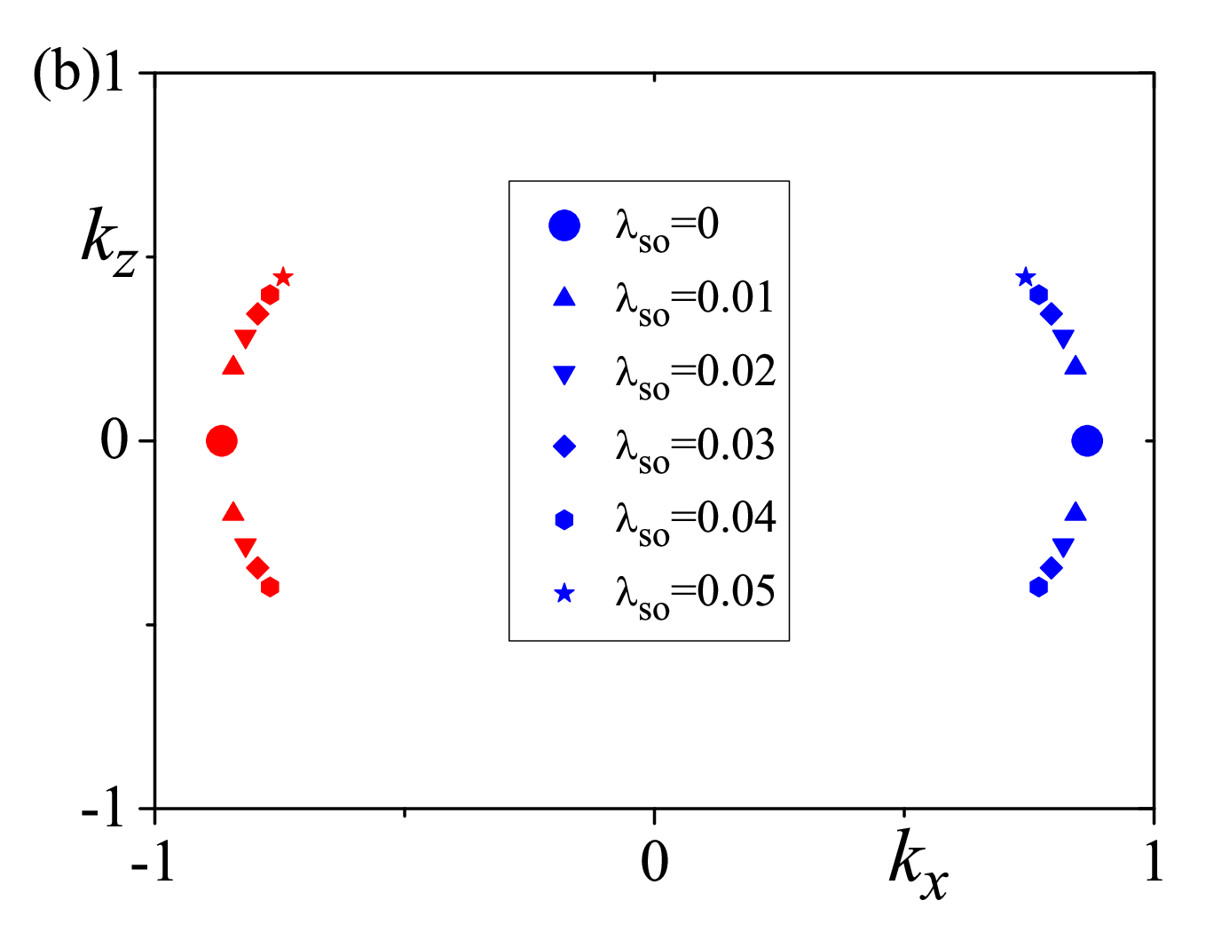
which harbors a pair of doubly-degenerate double-Weyl points at . When , the energy spectra of this Hamiltonian can not be analytically solved, thus we calculate it numerically. As shown in Fig.5, the pair of doubly-degenerate double-Weyl points are spilt into four pairs of Weyl points in the presence of weak spin-orbit coupling, with two pairs located at the plane, and the other two pairs located at the plane.

V Experimental estimations
V.1 Estimation of the modification to energy bands
The modification to energy bands by the driving can be evaluated by calculating the quantity , in which is the parameter of static Hamiltonian (see main article). As , where is the electric field strength, the quantity can be further rewritten as
| (48) |
For and , we adopt the experimental parameters in the pump-probe experiment[102], where meV, and V/m. For , we take the material candidate Cu3NPd to make an estimate. According to the band structure obtained by first principle calculation[54, 55], eV, and with Å[138], thus eVm2. Then
| (49) | |||||
Such a magnitude of modification can be readily observed in current experiments.
V.2 Estimation of Hall voltage in experiments
Due to the existence of monopole charges, anomalous Hall effect will show up in WSMs. At zero temperature and neutrality point (chemical potential ), the Hall conductivities are given by[20]
| (50) |
where and is the Levi-Civita symbol; and denotes the monopole charge and the -component of the momentum of the -th Weyl point, respectively.
Now we consider the NLSM Hamiltonian with cubic symmetry (see Sec.II). For a CPL incident in a general direction , the Hall conductivities can be obtained according to Eq.(50), which are
| (51) | |||||

Now we consider an experimental setup illustrated in Fig.6. In Fig.6, represents the current in direction and we will assume that it is distributed uniformly. denotes the spacing between current contacts, while and denote the length in the direction and the thickness in the direction (also the spacing between voltage contacts). Because the current is in the direction, will play no role in transport, so we restrict the CPL in the - plane in which naturally vanishes.
The resultant Hall voltage can be estimated as follows:
| (52) | |||||
Here we have assumed that for simplicity as the original static system has cubic symmetry. is the penetration depth, determined by , with the refraction index of the material, the permittivity of vacuum, the speed of light, and the absorption part of the optical conductivity, which only depends on the size of the nodal line, i.e., . Due to the cubic symmetry of the original Hamiltonian, is also assumed to be isotropic.
In the following, we also take Cu3NPd, a material candidate of NLSM with type-I crossing, as a concrete example to estimate the Hall conductivities and the Hall voltages. Cu3NPd crystallizes in the cubic perovskite structure with lattice constant Å[138]. First principle calculations found that the nodal-line size (diameter) is about , i.e., [54, 55]. For , the angle that creates double-Weyl points, we have
| (53) |
We do not find any experimental result of the refractive index of Cu3NPd, but for its parent material Cu3N, the refractive index is about in the visible light regime[139], and we take this value to estimate the penetration depth. Thus,
| (54) | |||||
For the dc conductivity of Cu3NPd, the room temperature value[140] is about . The value in the zero temperature limit is expected to be larger, and we assume as an estimation. We take m, nm, and mA, then a combination of Eq.(52), Eq.(53) and Eq.(54) gives mV, which is well within the capacity of current experiments.