Korshunov instantons in a superconductor at elevated bias current
Abstract
Even at zero temperature dissipation reduces quantum fluctuations and tends to localize particles. A notable exception is the nonlinear dissipation due to quasiparticle tunneling in a Josephson junction. It is well known that quasiparticle dissipation does not suppress tunneling of the superconducting phase difference between next-nearest metastable phase states even though tunneling to the nearest phase state is suppressed. The reason is that the dissipative action admits an instanton solution, the so-called Korshunov instanton. Here, we analyze this model at elevated bias current . We find that besides the known regime where the logarithm of the tunneling rate scales as there is novel regime with a scaling . We argue that the increased tunneling rate that derives from the elevated bias current is favorable for an experimental verification of the Korshunov instantons.
pacs
74.50.+r, 74.40.-n 85.25.CpI Introduction
Dissipative effects in quantum mechanics have been an object of research for a long time. With their simple model of quantum dissipation, Caldeira and Leggett popularized a linear and analytically trackable model to effectively describe dissipation in quantum systems [1, 2]. Despite the tremendous success of this simple model, it cannot describe all dissipative effects; for example, it does not describe quantization of the transported charge in a resistor built from a tunnel junction. To this end, the Ambegaokar-Eckern-Schön (AES) model was introduced modeling a superconducting tunnel junction that is subject to quasiparticle tunneling [3]. The latter introduces a dissipative term in the action that is periodic in the superconducting phase difference with a period of corresponding to the normal flux quantum. In Ref. 4, it was noted that due to quasiparticle tunneling the ground state is either a superposition of the phase localized in the even or odd minima of the Josephson potential. Remarkably, these superpositions are immune to the quasiparticle dissipation and survive even in the limit of strong dissipation. As a consequence, the phase ‘particle’ does not localize in one of the minima [5]. The action describing the quasiparticle tunneling admits instanton solutions, the so-called Korshunov instantons, that connect minima in the Josephson potential separated by . This results in a coherent tunneling amplitude between states localized in next-nearest minima and, consequently, the formation of bands. However, the band-width is exponentially small in the damping parameter and thus the experimental verification remains challenging.
In a different context, Korshunov instantons are important to understand charging effects of metallic islands connected to reservoirs via tunnel junctions [6, 7, 8, 9, 10]. Recently, the charging energy of a normal island has been measured as a function of the tunnel coupling [11]. However, to our knowledge, a direct observation of Korshunov instantons of the superconducting phase tunneling to the next-nearest minima is still missing. This observation would not only be interesting as an example where strong dissipation does not completely suppress tunneling but also because Korshunov instantons are related to coherent, paired phase slips which are of interest for example for the realization of parity protected qubits[12, 13, 14, 15]. Additionally, the system is an interesting example of dissipative quantum mechanics with a multitude of different regimes that can be accessed by simply changing the bias current; the regimes cover coherent quantum dynamics, even in the presence of strong dissipation, the case of a special incoherent relaxation due to quasiparticle tunneling, and more conventional Ohmic relaxation [16, 5].
In this work, we investigate the effect of an elevated bias current on Korshunov instantons at zero temperature. This is relevant because increasing the bias current raises the tunneling rate of the superconducting phase to the next-nearest minima of the potential that is the hallmark of the presence of strong quasiparticle dissipation and thus increases the chance of experimental verification of the theoretical results. We find that, apart from the low bias regime with , studied in Ref. 5, there is a novel regime at elevated bias current where . At even higher bias current, the quasiparticle nature of the dissipation becomes irrelevant and only tunneling to the next-nearest minima survives that is described by the conventional Ohmic model of Caldeira and Leggett. We discuss on the transition between the different regimes and propose an experimental method to measure the predicted decay rates.
The paper is organized as follows. In Sec. II, we introduce the setup and the theoretical model. In III, we provide a short introduction to the notation and the instanton method that we use throughout this work. In IV, we give a comprehensive derivation of the coherent tunneling amplitude before we proceed with the calculation of the incoherent tunneling rates in Sec. V. Note that these sections have some overlap with the work of Ref. 5. Section V includes our main result of the scaling of the tunneling rate at elevated bias current. Moreover, we discuss the transition between the coherent, incoherent, and conventional Ohmic regime. In VI, we propose a simple scheme on how to measure the incoherent tunneling rate before we end with our conclusions.
II Setup
For our analysis, we consider a current biased tunnel junction between two superconducting leads that is intrinsically subject to quasiparticle tunneling that acts as a dissipative element. This can be described by the AES model. In the Euclidean (imaginary time) path-integral formalism, its dimensionless action at zero temperature is given by[3]
| (1) |
where is the superconducting phase difference across the Josephson junction and its derivative with respect to the imaginary time . The first term describes the coherent superconducting circuit consisting of a Josephson junction with Josephson energy , where is the junctions critical current and the superconducting flux quantum. The capacitive energy due to the junctions capacitance is given by . The second term (quasiparticle action) corresponds to the dissipation due to quasiparticle tunneling. Its magnitude is connected to the effective shunt resistor . For small , the dissipative action can be expanded in a Taylor series so that it reproduces the Ohmic action described by Caldeira and Leggett. However, this approach neglects the periodicity of . The latter causes the action to stay invariant for a -phase shift corresponding to the tunneling of a normal flux quantum [17]. This refers to the fact that the quasiparticles are quantized single electrons and therefore do not feel a shift of a normal flux quantum.
In this work, we are interested in the regime where the dissipative action dominates with . Such a strong dissipation brings the system always into the semiclassical regime so that an instanton analysis is applicable. Interestingly, the quasiparticle action by itself can admit instanton saddle points without an additional kinetic or potential term. Therefore, the solution of , where is the first variation of the quasiparticle action, is an approximative saddle point of the full action . In Ref. 5, it was shown that there exists a solution for this equation, the Korshunov instanton , with arbitrary frequency , that connects not neighboring minima of the Josephson potential but next-nearest minima. For vanishing bias current , it is this instanton of the dissipative action that results in a coherent tunnel element between minima shifted by and leads to the formation of bands even in the presence of strong dissipation. However, the resulting bandwidth is small and difficult to tune and the effect of the pure coherent tunneling therefore is difficult to measure. The situation can be changed by applying a bias current . On one hand, this destroys the bands but on the other hand it introduces a dissipative incoherent tunneling rate where a phase particle located in one of the minima tunnels by to the next-nearest minimum. Additionally, the bias gives rise to ‘Ohmic’ decay into the next minimum for which the quasiparticle action acts as a simple Ohmic shunt. Contrary to intuition, at low bias current, the tunneling dominates the tunneling, i.e., the particle is more likely to tunnel to the next-nearest minimum than to the nearest minimum. While the tunneling vanishes at zero bias, the process transforms into the coherent tunneling element.
For the analysis, we introduce the dimensionless parameters
| (2) |
The normalized bias current gives a measure of how strong the potential is tilted. For , the tilt due to the bias is so strong that the minima in the potential vanishes. At this point, the particle classically slides down the potential landscape. The parameter describes the ratio between the capacitive kinetic energy and the Josephson potential energy. Without dissipation, it describes the quantum uncertainty of the phase with . The parameter describes the strength of dissipation. For large , the dissipation is strong and the phase becomes localized. Note that for , semi-classical methods are applicable even for .
III Saddle Point Approximation
In this section, we concisely describe the instanton method for analyzing tunneling problems. In the following sections, coherent tunnel elements as well as incoherent tunneling rates will be calculated. Both can be accomplished by evaluating the imaginary time path integral in Gaussian approximation around a saddle point of the action . In general, the action admits different saddle points with different physical meanings. Given a saddle point, the imaginary time propagator can be approximated as
| (3) |
Here, is defined as the solution of with appropriate boundary conditions, is the functional integration measure, while the subscript indicates that the path integral should be evaluated in Gaussian approximation around the extremum .
The action corresponds to expanded to second order in the fluctuations deviating from the extremal path. In particular, we set
| (4) |
with . The approximated action can be written as
| (5) |
where is the action directly evaluated at the extremal path . For the second equality, we have assumed that the fluctuation modes are eigenfunctions to the second variation satisfying
| (6) |
with eigenvalues and normalized to . With this, the integration measure can be chosen to be where is a normalization constant. Every positive leads to a Gaussian integral with the result
| (7) |
For an instanton solution , we have to deal with a zero eigenvalue that cannot be treated by the simple Gaussian integration above. Handling it correctly[18, 19] leads to the prefactor with[2]
| (8) | ||||
| (9) |
Here, the frequency denotes the plasma frequency and the factor incorporates the product of the three lowest eigenvalues including the zero eigenvalue. The zero mode is accounted for by the expression . The factor includes the eigenvalues with . Its leading behavior is determined by the asymptotics for . The correspond to the fluctuations around the constant path . They enter the equation when fixing the normalization .
To conclude this section, we shortly discuss the applicability of the semiclassical approximation above. It corresponds to the method of steepest decent that is applicable as long as is much larger than one. Additionally, within one potential well, the phase should be localized in the minimum. While this condition normally demands , it is always fulfilled in the case of strong dissipation as the dissipation localizes the phase difference across the Josephson junction.
IV Coherent Tunneling

Coherent quantum tunneling describes the Hamiltonian evolution of a system that connects localized states separated by a classically inaccessible barrier. This unitary evolution leads to quantum superposition of the particle in different potential wells. In our case, the system is mainly localized in the minima of the Josephson potential, i.e., at . This makes it possible to treat the minima of the cosine potential as sites of a linear lattice. The tunneling between different sites causes the formation of bands with a bandwidth equivalent to twice the tunneling matrix element. The bandwidth can be expressed by the imaginary time propagator evaluated at the so-called instanton . It is a saddle point of the action connecting two minima of the Josephson potential. It can be shown that the bandwidth is given by , where is the action evaluated at the instanton saddle point and originates from the Gaussian fluctuations around this instanton path [18].
IV.1 Instanton Action
We are going to determine the extremal action corresponding to an instanton that connects two minima of the Josephson potential. For this analysis, we are essentially following Ref. 5. The saddle point equation reads
| (10) |
An instanton solution to this equation is given by [5]
| (11) |
connecting a minimum of the -potential at with a next to nearest neighbor minimum shifted by at . It depends on the frequency that determines how fast the phase flips. The solution is in principle only a saddle point of the quasiparticle action and not of the full action . However, in the case , the quasiparticle action dominates the saddle point solution and thus even including the circuit action in Eq. (10) changes the instanton only perturbatively. Therefore, it is justified to insert the quasiparticle instanton into the action which corresponds to proceeding with first order perturbation theory. We find as resulting action on the instanton path
| (12) |
The action depends on so that we also need to extremize with respect to this parameter. We find a minimum of the action where is equal to the plasma frequency of the minimum with . At this minimum the instanton action becomes
| (13) |
IV.2 Instanton Prefactor and Result
The next step is the evaluation of the fluctuations to determine the prefactor . The explicit action of the fluctuation operator on the is given by
| (14) | ||||
| (15) |
where we separated the operator in circuit and dissipative contributions. By acting on the , these operators define a stationary Schrödinger equation with a non-local potential. Here, the imaginary time plays the role of the spatial coordinate. The lower eigenvalues are mainly determined by the dissipative action corresponding to bounded states in the potential. However, for the high energy modes, it is the kinetic energy term that dominates and gives rise to a continuum of states lying above the bounded spectrum. For ease of mode counting, we temporarily introduce a finite imaginary time interval with periodic boundary conditions, corresponding to nonzero temperatures. At the end, we send the interval to infinity again.
For low energies, only the dissipative action is relevant. The eigenvalue equation related to Eq. (15) is given explicitly as (for )
| (16) |
where the denotes the Cauchy principle value. In general such an equation is hard to solve. However, we obtain a zero mode for each free parameter of the instanton solution Eq. (11), which are in our case the imaginary time and the frequency . These zero modes generate a shift or dilation of the solution in imaginary time without changing the value of the action . The zero modes can be found by taking the derivative of the instanton path with respect to the corresponding free parameters. We find
| (17) |
both with eigenvalue ; the normalization fixed by .
It is well known that for Schrödinger like equations the number of nodes in the eigenfunction can be associated with the size of the eigenvalue, where the eigenfunction with the lowest number of nodes corresponds to the lowest eigenvalue [20]. For higher modes, the zero modes should be modulated in order to obtain more nodes [19]. For , we obtain approximately [5]
| (18) |
with the eigenvalue , where are the bosonic Matsubara frequencies. We incorporate the effect of by performing lowest-order perturbation theory with
| (19) |
We obtain , , and for the lowest three eigenvalues determining .
The calculation of we first consider only the kinetic term in (14) and treat the rest as a perturbation. The eigenfunctions of the kinetic operator are given by and with eigenvalues . By treating the rest of the action in first order perturbation theory, the eigenvalues at large are given by
| (20) |
The term proportional to originates from the fluctuations in the Josephson potential while is produced by the last term in (16). The -independent offset is generated by the first part of the first term in (16), whereas the integral without the principal part does not contribute for large because it is exponentially suppressed by the factor . For the normalization of we also need the eigenvalues corresponding to the fluctuations around the constant path . These are given by
| (21) |
and correspond to in Eq. (20) without the offset .
V Incoherent tunneling

Switching to a finite bias current , we render the minima in the Josephson potential unstable. Considering the Hamiltonian time evolution in this system, we cannot treat the minima of the Josephson potential as sites with a single level of a tight binding model as for the case of coherent tunneling. The evolution brings the initial state into a superposition of excited states of the neighboring minimum. Only the strong dissipation then localizes these state again in the local minimum. Such an evolution is called incoherent tunneling. For intermediate evolution times, this can be approximated as an exponential relaxation out of the original well and can be expressed by an imaginary part of the energy when starting in a single minimum. For this problem, the important object is not the instanton trajectory but the bounce . This is a cyclic trajectory connecting the minimum with a turning point and going back to its starting point as shown in the lower plot of Fig. 1. It can be shown[18] that in this case, the incoherent decay rate is given by ; here, is the action evaluated at the bounce trajectory and in (8) we have to replace by because of an occurring negative eigenvalue of the second variation, see below.
V.1 Bounce Action

We start this section with the discussion of the bounce action . In principle, as the quasiparticle action dominates, it is justified to find a saddle point of only the quasiparticle action and treat the circuit action in perturbation theory, as in the case of the instanton. However, there is also a bounce solution that is mainly determined by the circuit action. It corresponds to the tunneling of the phase difference through the barrier between the origin and the nearest neighbor minimum of the Josephson potential. In Fig. 2, this is indicated by the arrow labeled with . For such a trajectory, we can expand the quasiparticle action to second order so that it reproduces conventional Ohmic dissipation. Therefore, we call the decay due to this bounce solution in the following ‘Ohmic decay’. It results at low temperatures in the decay rate [16]. For small currents, this rate is lower than the rate of decay to the next-nearest minimum caused by the quasiparticle action. While it accounts for a phase slip, the quasiparticle bounce corresponds to a paired phase slip into the next-nearest minimum. Therefore, both processes can physically be distinguished and should be individually considered. In the following, we calculate the dominating rate of decay due to the quasiparticle tunneling.
The analytical solution to the saddle point problem of that fulfills the boundary conditions of the bounce is not known. However, we can construct an asymptotic saddle point by adding an instanton shifted by in imaginary time with an anti-instanton shifted by in the other direction resulting in the bounce path . This trajectory has the free parameters and , where the first describes how fast the phase switches in imaginary time and the second how long it stays in the shifted minimum before it returns. In the limit , becomes an exact saddle point of the dissipative action . Evaluating the whole action for this trajectory corresponds to first order perturbation theory in the circuit action . This approach leads to a bounce action still depending on the two free parameters of the bounce. To find the approximate saddle point, we need to extremize with respect to these parameters. We find two distinct regimes: the first one corresponds to the regime found in Ref. 5 that is valid as long as stays approximately constant. We denote the regime at small bias current by (i). In this regime, we find
| (24) |
resulting in the action
| (25) |
At elevated bias currents , we find a second novel regime in which the frequency starts to decay . In this regime, we have to minimize in both parameters and , see App. A for more information. The resulting saddle point solution is given by
| (26) |
with
| (27) |
As , the term , which is the quasiparticle action contribution of two infinitely separated instantons, always dominates. This is in agreement with our assumption that the dissipative term approximately determines the saddle point. If we exceed the critical current , the extremum for is found at and therefore the bounce of the dissipative action approaches the constant solution that stays in the minimum of the Josephson potential. In Fig. 3, we compare Eq. (25) and Eq. (27) to the value of at the saddle point that we obtained numerically.
V.2 Bounce Prefactor and Result

To find the -tunneling rate, the remaining task is to calculate the prefactor that represents the quantum fluctuations on top of the bounce path. The procedure is similar to the calculations for the instanton, however with some complications added. First of all, we have to evaluate the fluctuation operator at the bounce trajectory so that the eigenvalue equation does not take the simple form (16). We can approximate the exact fluctuation operator of by the form
| (28) |
valid for . It corresponds to the instanton eigenvalue equation (16) with a potential at each positions of the constituting instantons. For large , the potential are well-separated, so that the eigenmodes are expected to be superpositions of the instanton eigenmodes.
For example, for the low energy eigenvalues needed in the factor , we can make the ansatz of the even and odd superposition of the shifted instanton zero modes
| (29) | ||||
where and the new normalization is given by .
By comparing (29) with the derivative of the bounce in respect to the imaginary time we see that the odd superposition indeed corresponds to the real zero mode. This zero mode generates a shift of the whole bounce trajectory in imaginary time. Moreover, approximately (up to ), the even superposition is a zero mode of the quasiparticle action, too. It is a so-called breathing mode and generates a shift of the two instanton parts of the bounce in two different directions, changing the size of the bounce. It can also be obtained by taking the derivative of the bounce in respect to . Counting the numbers of nodes we recognize that the zero mode has one node, while the even mode has no nodes. Therefore, the even eigenvalue has to be negative. For a negative eigenvalue the naive Gaussian fluctuation approximation breaks down. However, it is this negative eigenvalue that gives rise to the imaginary part of the energy that corresponds to the decay rate [18].
The degeneracy between the even and odd mode is lifted if we perturbatively consider the fluctuations of the circuit action. However, here we cannot take the simple approach as in (19) for the instanton. We encounter the problem that we do not know the eigenfunctions accurately enough for this treatment. The eigenfunctions of the quasiparticle action are a good approximation to the real eigenmodes away from the position of the instantons. However, close to these positions the eigenmodes are subject to ‘fast’ modulations that are not included in lowest order perturbation theory.
In Fig. 4, we show the Josephson potential for the fluctuations around the bounce and the even mode to visualize the problem. The eigenfunction plotted as the dashed line is clearly not a ground state for the potential close to the points with . The missing fast modulations are irrelevant for the quasiparticle action but change the contribution by the Josephson potential already on the order of . However, the splitting between the even and odd mode is of the order and thus we have to apply a modified procedure.
The idea is to directly calculate the splitting between the two lowest eigenvalues and instead of finding their absolute values. Knowing that for the exact solution of the problem, we obtain . It is possible, to calculate without accurate knowledge of the wavefunctions close to the instanton position. For that we define , , and with the Josephson potential evaluated at the bounce. We can rewrite the circuit fluctuation operator as
| (30) |
In the expression
| (31) |
for the first order perturbation, we make use of the fact that for the zero mode. This removes the terms that are localized in the dangerous region around the instanton position. Additionally, for the second equality, we have left out terms proportional to that are higher order in .
For the modes with more than one nodes (), the accuracy of the conventional perturbation theory is sufficient. By using the odd superposition of the shifted instanton eigenmodes, we can estimate the third eigenvalue as . The expression for the normalization due to the zero mode reads . As a result, we obtain the prefactor
| (32) |
In order to calculate , we still have to determine the higher eigenvalues corresponding to . The high-energy eigenmodes are still approximatley given by the eigenfunctions of the kinetic operator. We obtain the corresponding eigenvalues by inserting the second variation (28) of the bounce into the expression (20). We find the result
| (33) |
where the factor in the last term compared to (20) originates from the fact that there are two instantons contributing to the bounce. Plugging (33) into (9) yields (for )
| (34) |
With the results (33), (34), and the ones in Sec. V.1, we are in the position to evaluate the decay rate for the two regimes identified above. For low bias current , the rate is given by[21]
| (35) |
For elevated currents with , the decay rate is given by
| (36) |
The crossover from the result (35) to (36) that we describe in more details below as well as the decay rate (36) at elevated bias current are the main results of the present work.
V.3 Regimes and Crossovers
In this section, we will discuss the crossovers between the regimes identified above. Without bias current, the system forms bands due to dissipation mediated coherent tunneling. We call this regime the ‘coherent regime’, see Fig. 5. The amplitude then defines a tunneling matrix element for a phase slip. Increasing the bias current , more than a single state in the well separated by becomes energetically accessible and the coherent tunneling transforms into an incoherent relaxation. A quantitative criterion for the crossover from the coherent to the incoherent regime can be defined by . This gives an estimate whether we can treat the position of the bounce as a classical variable or whether quantum fluctuations have to be taken into account. As long as the quantum fluctuations of are smaller than the optimal separation between the instantons , the bounce and therefore incoherent tunneling is an appropriate description. If the fluctuations in increase, the system is more accurately described by a gas of individual instantons giving rise to coherent tunneling elements. Depending on the parameters, tuning up leads in general to a crossover of the action to the regime (i) with a scaling of and then to the regime (ii) with a scaling . However, for , the regime (i) is never realized and the system directly crosses over from the coherent regime to the regime (ii). From the crossover criterion above, we obtain the approximate expressions for the crossover (at fixed )
| (37) |
in the regime and
| (38) |
in the regime . At the rate of phase slips generated by the Ohmic bounce solution is of the same order as the quasiparticle decay . However, the two processes are physically distinguishable so that they can be individually measured; see also below. At a bias current above , the bounce connecting two minima separated by vanishes such that only Ohmic dissipation is present in this regime.

VI Measurement
As demonstrated above, Josephson junctions with strong quasiparticle dissipation admit many interesting properties that can be subject of an experimental investigation. The simplest approach to observe effects of the special (non-linear) form of the dissipation due to quasiparticle tunneling is to measure the incoherent tunneling. Measuring the coherent tunneling directly is challenging due to the small bandwidth exponentially suppressed in without any additional tuning parameter. Therefore, we propose to measure paired phase-slip events and compare the resulting rates to the expressions (35) or (36).
The key idea for the experimental observation of the paired phase slips is to raise the bias as much as possible, i.e., smaller than but still in its vicinity, in order to increase the rate of paired phase slips. An important requirement for the experimental setup in order to be able to operate at elevated bias current is the possibility to distinguish between double and single phase slips. The reason is that at elevated bias current, the rate of unpaired phase slips can already dominate the rate of paired phase slips. Additionally, even if we can distinguish between the two processes, we need to make sure that the process can be uniquely associated with the periodic quasiparticle tunneling while the process is caused solely by the conventional Ohmic tunneling. The latter process does not necessarily end up in the nearest minimum. If the momentum, i.e., the kinetic energy, of the phase difference is to large it may not be retrapped after the tunneling but it can classically go on over the next potential hill and end up in the following minimum. Especially after the point at which the Ohmic tunneling rate exceeds the quasiparticle rate or respectively it is not possible to distinguish between the two processes anymore. Therefore, it is best to keep the capacitance small so that the dissipation always brings the Ohmic phase slips to rest in the next minimum. Additional it is advantageous to use small because it allows to consider systems with smaller without making the ratio too large. Smaller then keeps the exponential suppression of the phase-slip rate low.
An approach that can satisfy the above requirements is to include the Josephson junction into a loop with inductance or alternatively build an asymmetric SQUID so that one Josephson junction serves as an inductance; see Ref. 22, 23 for a recent experimental setup. With a magnetic bias, it is possible to add an external flux in the loop that takes the role of the bias current. Placing the circuit in a transmission line, the number of flux quanta in the loop can be measured non-destructively by a flux dependent shift of the transmission phase of the input and output signal into the transmission line. This flux dependent shift in the transmission phase directly indicates when a or a -event has happened. By recording these events over a given measurement time, the resulting rates can be compared with the results (35) or (36). Theoretically, the setup corresponds to introducing the additional term to the circuit action with induction . In this setup, the bias current is given by the term linear to with . The additional quadratic contribution simply changes the bias current according to . This takes care of the fact that a quadratic potential needs already an external flux of until the minimum at becomes unstable for the Korshunov decay channel while without the quadratic confinement an infinitesimal bias is already enough to render the minimum unstable. A similar setup has been used in Ref. 23 to measure the interference between phase slips in two parallel nanowires. It indicates that the quasiparticle tunneling in nanowires is strong and therefore these wires are a potential candidate for such an experimental setup. Note that there are also other potential experimental probes that can detect changes in flux. For example, flux dependent absorption process could be used to measure the rate of paired phase slips.[24, 25]
VII Conclusion
In conclusion, we have shown that the coherent dissipation due to quasiparticle tunneling over a Josephson junction in a superconductor can be probed by the measurement of 4 phase-slip events. These -phase slips are caused by Korshunov instantons probing the specifics of the nonlinear dissipation due to quasiparticles. We have identified a novel regime at elevated bias current that leads to a substantially increased rate of 4 phase slips. This is important as the low rate is one of the main reasons why paired phase slips are challenging to measure. We have discussed the different crossovers between the coherent regime and the incoherent regimes. In addition, we have proposed a measurement scheme for the detection of the paired phase slips; fixing the bias current slightly below a critical current and working with a small capacitance , corresponding to a large charging energy, offers the best chance to observe paired phase slips due to the increased rates. We hope that our analysis helps to guide the experimental effort to directly observe Korshunov instantons as paired phase slips of the superconducting phase.
VIII Acknowledgments
The authors acknowledge support from the Deutsche Forschungsgemeinschaft (DFG) under grant HA 7084/2-1.
Appendix A Extremizing the action in different regimes
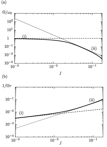
In this appendix, we provide details for the extremizing the action to find the regime (i) corresponding to equations (24) and (25) and regime (ii) corresponding to equations (26) and (27). The action evaluated at the bounce trajectory and consistently expanded for large up to second order reads
| (39) |
In Fig. 6, we show an example of the resulting optimal parameters calculated by a numerical optimization of the action above with respect to and . It clearly shows two distinct regimes with different power law behaviors. The first regime corresponds to regime (i) with a constant while the second regime corresponds to (ii) with decaying . The crossover is numerically found to be at , see below.
An analytic expression valid in the regime (i) can be found by assuming and optimizing (39) with respect to the single parameter . In this case, only the two last terms in (39) contribute. This yields Eqs. (24) and (25) for the optimal point.
By increasing the bias current, the assumption fails to hold as the inverse size of the instanton starts to decline with raising bias current . As a result the term starts to become relevant. The point at which this happens can be estimated by comparing it to one of the two last terms, e.g., . With [from (24)], we obtain the estimate for the crossover current as before.
So for , the parameters and in the action have to be simultaneously optimized. Not all terms of the action (39) are relevant. In the first term, we can neglect the term proportional to as . In the last term, only the term proportional to is relevant as . Thus, the effective action in the regime (ii) reads
| (40) |
Extremizing this action with respect to the parameters and is straightforward and leads to the results of Eq. (26). Inserting the optimized parameters into Eq. (40) yields the simple expression for the action
| (41) |
that is equivalent to (27). For bias currents , the accuracy of (27) can be increased by including small corrections to the -dependence with first order perturbation theory. This corresponds to inserting the optimized values and from Eq. (26) into the full action (39).
References
- [1] A. O. Caldeira and A. J. Leggett, Influence of dissipation on quantum tunneling in macroscopic systems, Phys. Rev. Lett. 46, 211 (1981).
- [2] U. Weiss, Quantum Dissipative Systems, Series in modern condensed matter physics (World Scientific, 2012).
- [3] V. Ambegaokar, U. Eckern, and G. Schön, Quantum dynamics of tunneling between superconductors, Phys. Rev. Lett. 48, 1745 (1982).
- [4] F. Guinea and G. Schön, Coherent charge oscillations in tunnel junctions, Europhys. Lett. 1 (11), 585 (1986).
- [5] S. E. Korshunov, Coherent and incoherent tunneling in a Josephson junction with a “periodic” dissipation, JETP Lett. 45, 434 (1987).
- [6] S. V. Panyukov and A. D. Zaikin, Coulomb blockade and nonperturbative ground-state properties of ultrasmall tunnel junctions, Phys. Rev. Lett. 67, 3168 (1991).
- [7] Yu. V. Nazarov, Coulomb blockade without tunnel junctions, Phys. Rev. Lett. 82, 1245 (1999).
- [8] A. Altland, L. Glazman, A. Kamenev, and J. Meyer, Inelastic electron transport in granular arrays, Ann. Phys. (NY) 321, 2566 (2006).
- [9] A. T. Bollinger, A. Rogachev, and A. Bezryadin, Dichotomy in short superconducting nanowires: Thermal phase slippage vs. Coulomb blockade, Europhys. Lett. 76 (3), 505 (2006).
- [10] M. Titov and D. B. Gutman, Korshunov instantons out of equilibrium, Phys. Rev. B 93, 155428 (2016).
- [11] S. Jezouin, Z. Iftikhar, A. Anthore, F. D. Parmentier, U. Gennser, A. Cavanna, A. Ouerghi, I. P. Levkivskyi, E. Idrisov, E. V. Sukhorukov, L. I. Glazman, and F. Pierre, Controlling charge quantization with quantum fluctuations, Nature 536 (2016).
- [12] B. Douçot and J. Vidal, Pairing of Cooper pairs in a fully frustrated Josephson-junction chain, Phys. Rev. Lett. 88, 227005 (2002).
- [13] L. B. Ioffe and M. V. Feigel’man, Possible realization of an ideal quantum computer in Josephson junction array, Phys. Rev. B 66, 224503 (2002).
- [14] S. Gladchenko, D. Olaya, E. Dupont-Ferrier, B. Douçot, L. B. Ioffe, and M. E. Gershenson, Superconducting nanocircuits for topologically protected qubits, Nature Phys. 5 (1), 48 (2009).
- [15] M. T. Bell, J. Paramanandam, L. B. Ioffe, and M. E. Gershenson, Protected Josephson rhombus chains, Phys. Rev. Lett. 112, 167001 (2014).
- [16] S. E. Korshunov, Quantum-mechanical tunneling with dissipation in a sloping sinusoidal potential, Sov. Phys. JETP 65, 1025 (1987).
- [17] J. Ulrich and F. Hassler, Dual approach to circuit quantization using loop charges, Phys. Rev. B 94, 094505 (2016).
- [18] S. Coleman, The Uses of Instantons, pp. 805–941 (Springer, Boston, 1979).
- [19] A. I. Larkin and Yu. N. Ovchinnikov, Quantum-mechanical tunneling with dissipation. The pre-exponential factor, Sov. Phys. JETP 59, 420 (1984).
- [20] L. D. Landau and E. M. Lifshitz, Quantum Mechanics, vol. 3 of Course of Theoretical Physics (Pergamon Press, London, 1958).
- [21] This result is given in Ref. 5. Here, we correct the prefactor.
- [22] A. Belkin, M. Brenner, T. Aref, J. Ku, and A. Bezryadin, Little–parks oscillations at low temperatures: Gigahertz resonator method, Appl. Phys. Lett. 98 (24), 242504 (2011).
- [23] A. Belkin, M. Belkin, V. Vakaryuk, S. Khlebnikov, and A. Bezryadin, Formation of quantum phase slip pairs in superconducting nanowires, Phys. Rev. X 5, 021023 (2015).
- [24] F. Chiodi, M. Ferrier, K. Tikhonov, P. Virtanen, T. T. Heikkilä, M. Feigelman, S. Guéron, and H. Bouchiat, Probing the dynamics of Andreev states in a coherent Normal/Superconducting ring, Sci. Rep. 1, 3 (2011).
- [25] B. Dassonneville, M. Ferrier, S. Guéron, and H. Bouchiat, Dissipation and Supercurrent Fluctuations in a Diffusive Normal-Metal Superconductor Ring, Phys. Rev. Lett. 110, 217001 (2013).