Cooling of chiral heat transport in the quantum Hall effect graphene

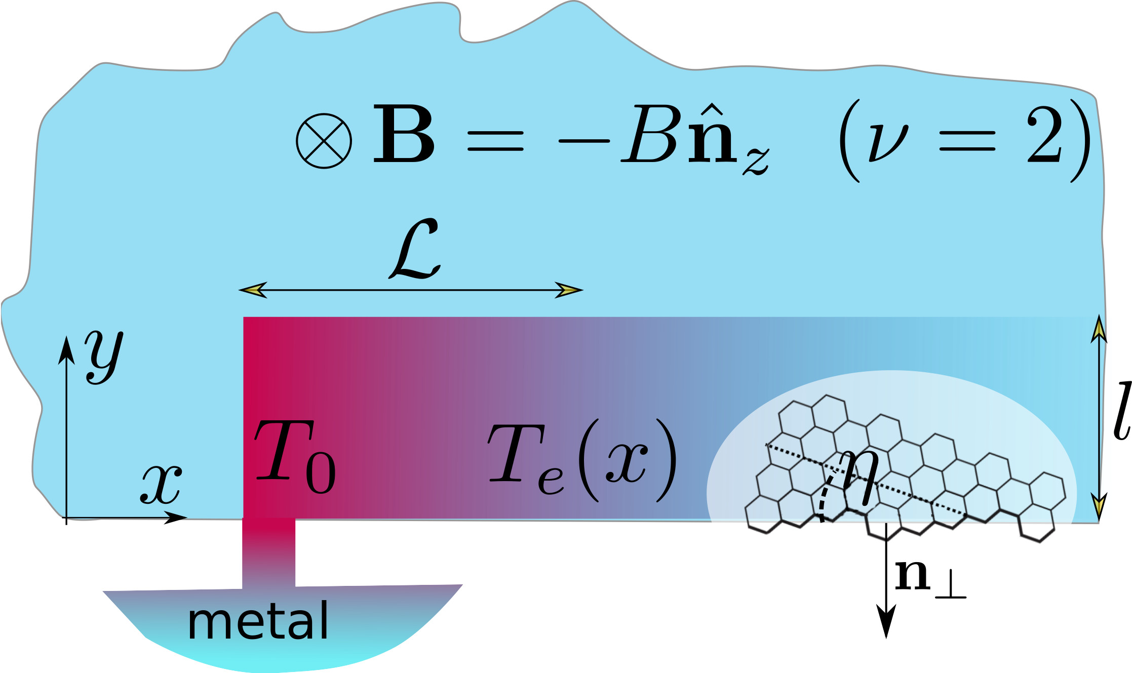
Graphene offers a promising material platform for the realisation of metrological resistance standard based on the phenomenon of Quantum Hall Effect (QHE) [1, 2, 3, 4, 5, 6, 7, 8, 9, 10, 11]. Precision metrology requires wide QHE plateux, such as observed at filling factor $\nu=\pm 2$ in epitaxial graphene on SiC[7, 10], and the largest possible breakdown current. The breakdown of QHE is triggered by the unavoidable hot spots [3, 12, 13] formed at the points where current is injected into the 2D electron gas from a normal metal contact. Hot electrons propagating from the hot spot to the potential contacts used in the QHE measurements spoil the precision of QHE resistance quantization [14]. In the QHE regime, electron energy spectrum is gapped inside the 2D structure, while the edge states [15, 16, 17, 18] carry non-equilibrium electrons. The chiral nature[15, 16] of edge states means that electrons propagate in only one direction, making the heat transport uni-directional, Fig.1, with the direction of the drift reversed upon reversal of magnetic field, ${\bf B}=-B\hat{\bf n}_{z}$. Chiral heat transport was experimentally observed both in semiconductor heterostructures [19] and in graphene [20]. Here, we propose a theory describing the temperature profile formed by the competition of chiral heat transport and acoustic-phonon-mediated cooling of electrons in the QHE edge states in graphene with filling factor $\nu=\pm 2$, for which the gap between LLs is the widest.

To model edge states in graphene, we use Dirac equation for electrons with generic boundary conditions [21, 22, 23] that provide zero value for the current across the edges and satisfy the time-inversion symmetry requirement at ${\bf B}=0$,

Here, $\sigma_{i}$ and $\tau_{i}$ are Pauli matrices acting separately on sublattice ($A,B$) and valley ($\pm K$) components of a 4-spinor, $\Psi^{T}=(\Psi_{KA},\Psi_{KB},\Psi_{-KB},-\Psi_{-KA})$, describing the electron amplitudes on sublattices $A$ and $B$ in the valleys $\pm K$. Generic boundary conditions in Eq.(1) are parameterized by two unit vectors, $\bm{m}$ and ${\bm{n}}\perp{\bf n_{\perp}}$, where $\bf{n}_{\perp}$ is normal to the edge in the 2D plane of graphene, Fig.1. Both $\bm{m}$ and $\bm{n}$ depend on the microscopic features of the edge in a particular sample. In particular, deviations of $\bm{m}$ from $\hat{\bf n}_{z}$ reflect the probability of inter-valley scattering upon specular reflection of an electron arriving at the incidence angle $\theta$ to the edge,

Vector $\bm{m}$ also accounts for the crystallographic orientation, $\eta$, of the edge: for zigzag edge ($\eta=\frac{\pi}{2}$) ${\bm{m}}=\hat{\bf n}_{z}$, for the armchair edge ($\eta=0$) ${\bm{m}}=\hat{\bf n}_{x}$ with $\phi=\pm\frac{\pi}{2}$. For straight edges, by exploiting valley degeneracy in Eq.(1) boundary conditions with different ${\bm{m}}$’s can be reduced by a unitary transformation in valley space to the ones with ${\bm{m}}=\hat{\bf n}_{z}$, thus, leaving all the sample-specific microscopic features of the edge incorporated in a single parameter $\phi$. For example, $\phi=0$ corresponds to an idealised nearest-neighbour-hopping model of zigzag edge with equal on-site energies on carbons, which imposes an artificial electron-hole symmetry on the electronic spectrum [24, 25, 26, 27, 28]. To compare, $\phi=\pm\pi/2$ correspond to the ’infinite-mass’ boundary condition for Dirac fermions [29], due to the sublattice symmetry breaking by a staggered potential, $\Delta\,\sigma_{z}\otimes\tau_{z}$, with $|\Delta|\to\infty$ at the edge. According to Ref. [22], boundary parameter $\phi$ can be related to staggered potential $-\Delta\sigma_{z}\otimes\tau_{z}$ ␮on $2N$ rows at a zigzag edge, as $\cos\phi␪=\frac{1+\sinh(\kappa)\sinh(\kappa+2N\Delta/t)}{\cosh(\kappa)\cosh(\kappa+2N\Delta/t)}$, with $\sinh\kappa␬=␮\Delta/(2t)$ and $t$ being the nearest-neighbour hopping in the tight-binding model. The boundary parameter $\phi$ also determines a phase shift, $\gamma_{\xi}=\pi+2\,\arctan\frac{\sin\theta\,(\cot(\phi/2))^{\xi}}{\xi-\cos\theta\,(\cot(\phi/2))^{\xi}}$, of a plane wave upon specular reflection of an electron arriving at the incidence angle $\theta$ to the edge at ${\bf B}=0$. Note that the armchair edge boundary condition is reduced to $\phi=\pm\pi/2$ (after the abovementioned unitary transformation in the valley space). In general, a non-zero $\phi$ determines the dispersion of the edge states characteristic for graphene edge at $B=0$,

where a valley-specific requirement $\xi p\cos\phi>0$ ($\xi=\pm 1$ for $\pm K$ valleys) guarantees confinement of evanescent states near the edge, $\Psi_{\xi}=\left[\begin{array}[]{c}\xi\\ \left(\tan\frac{\phi}{2}\right)^{\xi}\end{array}\right]e^{-\xi py\cos\phi+ipx}$.

To analyse the edge state problem (1) for the geomery of the edge shown in Fig. 1 ($x/y$ axes chosen along / perpendicular to graphene edge) and an arbitrary choice of $\phi$ and ${\bm{m}}$, we employ a unitary transformation,

which adjusts the sublattice composition of spinors in Eq.(1) to the choice of the coordinate system, simplifying the form of boundary condition by rotating $\bm{m}$ (to the angle $\widehat{{\bm{m}}\hat{\bf n}}_{z}$) to $\hat{\bf n}_{z}$ axis. Then, we use Landau gauge ${\bf A}=(By,0)$ for magnetic field ${\bf B}=-B{\bf\hat{n}}_{z}$, seeking solutions in the form of $\Psi^{\prime}(x,y)=e^{ipx}\psi(y)$, where $\psi^{T}=(\psi_{+A},\psi_{+B},\psi_{-B},-\psi_{-A})$. Now, it is convenient to rewrite the Dirac equation and its boundary conditions in a Schrödinger-like form using amplitudes $\chi_{+1}\equiv\psi_{+A}$ and $\chi_{-1}\equiv\psi_{-B}$ on one sublattice only,

where $\xi=\pm 1$, and $l=\sqrt{\frac{\hbar}{eB}}$ is a magnetic length.

Numerical solution of Eq.(3) produces spectra $E(p)$ for electrons near the edge shown in Fig.2 for various values of $\phi\in[0,\frac{\pi}{2}]$. Spectra for inverted, $\phi\to-\phi$, values of the boundary condition parameter can be obtained from those shown in Fig. 2 by changing $E(p)\to-E(p)$, and spectra for $\phi\to\pi+\phi$ by swapping $\chi_{+}$ and $\chi_{-}$. In Fig.2, one can recognize the 2D bulk Landau levels (LLs) at $p<0$, transforming into the edge states near $p=0$ The sublattice composition of the corresponding wave functions is shown in Supplementary Materials (SM) S1. Near the edge, the LLs resonantly mix with the edge states of Dirac electrons in graphene, Eq.(2), whose spectrum and valley composition depend on $\phi$. This mixing determines three parametric intervals for the edge states at $E_{F}=\frac{\hbar v}{\sqrt{2}l}$, which is the optimum choice of Fermi energy for developing QHE devices¹¹ 1 Moving $E_{F}$ within the gap introduces no qulitative changes.:

1. I)

   $\frac{\pi}{6}<\phi<\pi$ (and $\frac{7\pi}{6}<\phi<2\pi$), where there is one chiral edge state at the Fermi level, whose wave-function is a mixture of LLs and the evanescent mode present for $B=0$ for either $\chi_{+}$ or $\chi_{-}$ (in only one “valley”).

2. II)

   $0<\phi\lesssim\frac{\pi}{8}$ (and $\pi<\phi\lesssim\frac{9\pi}{8}$), where there are three edge modes. Two of these modes (one for $\chi_{+}$ and the other for $\chi_{-}$) are the counterpropagating evanescent modes with $\psi\propto e^{-\frac{y}{\sqrt{2}l}|\cot\phi|}$ confined at a short distance, $\lambda_{\phi}\sim\sqrt{2}l\tan\phi$, near the edge. Due to a strong confinement, $\lambda_{\phi}\xrightarrow[\phi\to 0]{}0$, these modes have suppressed scattering into the LL edge state. Note that, for $\phi\to 0$, a stronger confinement of evanescent modes would suggest a stronger intervalley scattering on atomically sharp edge disorder, localizing the counterpropagating evanescent modes.

3. III)

   $\frac{\pi}{8}\lesssim\phi\lesssim\frac{\pi}{6}$ (and $\frac{9\pi}{8}\lesssim\phi\lesssim\frac{7\pi}{6}$ ), characterized by two additional counterpropagating modes $\chi_{-}$($\chi_{+}$) with strongly overlapping wave-functions and one chiral mode $\chi_{+}$($\chi_{-}$). In this case, “intra-valley” scattering would lead to localization of pairs of $\chi_{-}$($\chi_{+}$) edge states.

As to the phonons, the feature of graphene coupled by van der Waals forces to the underlying substrate with a non-commensurate lattice is that vibrational properties in graphene lattice are only weakly perturbed by the substrate[31]. Hence, a graphene flake can be described as a membrane with free edges, where vanishing of stress tensor components in the direction ${\bf n}_{\perp}$ results in a zero deformation potential at the edge. This should be contrasted to graphene with clamped edges, where the displacement vector field of graphene is set to zero at the edge. In principle, both the longitudinal (LA, with displacement field ${\bf u}\parallel{\bf q}$) and the transverse (TA, with ${\bf u}\perp{\bf q}$) acoustic phonons in graphene could be emitted by hot electrons in the edge states. Those are coupled to electrons via a potential,

with [32, 33, 34, 35, 36, 37] $g\approx 20\,{\mathrm{eV}}$ and $g^{\prime}\approx 2\,{\mathrm{eV}}$ (since graphene is in the incompressible QHE plateau state, we use the unscreened value of the deformation potential coupling). As $g^{\prime}\ll g$, we base our analysis on emission of LA phonons provided by deformation potential with the constant $g$. Note that flexural phonons couple quadratically to electrons, allowing only for two-phonon processes that are negligible at low lattice temperatures [38]. Also, we find [Table 1 in Supplementary Materials (SM)] that the edge state velocities, $v_{e}=\left.\frac{\partial E(p)}{\partial p}\right|_{E=E_{F}}$, are much higher than the speed of longitudinal sound in graphene [39], $s\approx 2.1\cdot 10^{4}\rm m/s$; therefore, phonons are emitted with the wave vectors almost perpendicular to the edge, ${\bf q}=-q{\bf n}_{\perp}$. This feature of electron-phonon (e-ph) interaction in the edge states simplifies the description of their cooling kinetics. In particular, for the samples where parameter $\phi$ belongs to Interval I, where there is only one edge mode at $E_{F}=\frac{\hbar v}{\sqrt{2}l}$ for $\nu=2$, the e-ph interaction has the form,

where $b_{\bf q}^{\dagger}$ ($b_{\bf q}$) and $a_{p}^{\dagger}\,(a_{p})$ are the creation (annihilation) operators of LA phonons and of edge state electrons; $\rho\approx 7.6\cdot 10^{-7}\,{\rm kg/m^{2}}$ is graphene mass density. Here, the form factor,

takes into account the form of the edge state wave function and the phonon displacement field near the edge: for the free edge the phonon displacement mode behaves as $u_{y}\sim\cos(qy)$, leading to a deformation potential $V\sim q\sin(qy)$. For the states marked by dots in Fig. 2, the form factor $A(q)$ has the following characteristic asymptotics,

values of parameters $r_{0}$ and $\alpha_{0}$ are listed in Table I of SM.

Edge state electrons cool down while drifting along the edge. Assuming that, locally, their equilibration due to Coulomb interaction is fast, electrons’ distribution can be described using a Fermi function with a local temperature $T_{e}(x)$. We note that equilibration of edge channels has been shown to be non-thermal at longer time scales [40] due to integrability, but at the comparable time scales the phonon emission becomes important, breaking the integrability. We also find that for a slow thermalization of edge state electrons, their distribution formed in the course of cooling by phonon emission is almost indistinguishable from thermal, see SM S2. The cooling power (per unit length) provided by the phonon emission by the edge state electrons is

Here, $T$ is graphene lattice temperature, $T_{e}$ is the temperature of electrons in the edge state, and a factor,

accounts for all phonons emitted at various energies $\hbar\omega={\epsilon}T_{e}$, with $n_{B}({\epsilon})=\left[e^{{\epsilon}}-1\right]^{-1}$. The temperature scale,

is determined by the energy of phonons with $q\sim 1/l$. It marks a crossover between the two regimes: the high-temperature regime, $T_{e}\gg T_{*}$, where wavelengths of typical emitted phonons are smaller than $l$, $ql>1$, and a low-temperature regime, $T_{e}\ll T_{*}$, where $ql<1$. Then, for $T\ll T_{e}$, we find

For Interval II, the slow counter-propagating modes (seen in Fig. 2) provide additional cooling power. Since the spatial scale of their wave-functions is reduced to $l\tan\phi$, and their velocity is reduced to $v|\sin\phi|$, their cooling power is described by the same Eq.(5), but with increased $T_{*}\to T_{*}|\cot\phi|$. This leads to the extended range of low-temperature asymptotics, giving a small correction to cooling power

which rapidly grows to a dominant term at $T_{e}>T_{*}\cot\phi$. In the latter case, the equilibration between the edge channels shortens the cooling length. For Interval III, Eq.(7) can only give the lowest bound for the cooling efficiency, as phonons can be emitted by both intra- and inter-edge-state transitions.

All this leads to the equation for the temperature profile $T_{e}(x)$ along the edge,

where $C_{e}=\frac{\pi T_{e}}{6\hbar v_{e}}$ is specific heat of a 1D Fermi gas, $v_{e}$ is velocity of the fastest propagating edge channel, and $C\geq C_{e}$ is a full specific heat including the contributions from localized states at the edges. The validity of this equation for Intervals II and III is provided by cancellation of $C_{e}v_{e}$ contributions from the counter-propagating edge states and assuming that temperature equilibration between the edge channels is fast. If inter-channel equilibration is slow, then the effect of additional edge channels can be neglected. In the steady state, $\partial_{t}T=0$, this reduces to

Also, for comparing our results to the experimental data from Ref.20, it is convenient to characterize cooling by a differential cooling length, ${\cal L}(T_{e})$, defined as,

Solving Eq.(8), we find exponentially fast temperature decay at high temperatures, with $\gamma=\frac{g^{2}r_{0}^{2}eB}{2\pi\hbar^{2}\rho v_{e}^{2}s}$, and a slow power-law low-temperature tail:

The crossover between the two asymptotical regimes, from the fast decay at $T>T_{*}$ to the long tail at $T<T_{*}$, is illustrated in the inset of Fig.3(a), and the values of high-temperature cooling length,

are plotted in Fig. 3(b). It is interesting to note that reversing magnetic field does not change the values of the cooling length ${\cal L}$, which should be, now, applied to the hot electrons drifting in the opposite direction. However, changing $\nu=2$ to $\nu=-2$ by changing polarity of doping, would be equivalent to swapping $\phi\to-\phi$ in Fig.3(b), resulting in a different cooling length ${\cal L}$ for n- and p-doping of the same sample when $\phi\neq 0,\pm\frac{\pi}{2}$.

In the recent experiments on the chiral heat transport along the QHE edges in graphene [20], the temperature decay length ${\cal L}$ has been measured for the filling factor $\nu=-2$ at $B=16$ T, resulting in ${\cal L}_{exp}\approx 22\rm\mu m$. Estimates, based on the theory of phonon-assisted scattering in semiconducting heterostructures[41] have led the authors of Ref. 20 to refute the acoustic phonon cooling mechanism, leaving their results unexplained ²² 2 Here, we neglect the evaporational cooling by emission of hot electrons into the bulk Landau levels, as it is suppressed by the Boltzmann factor $e^{-\hbar v/(2lk_{B}T_{e})}$. For $B=16$ T $\hbar v/(2lk_{B})=840$ K, making this mechanism redundant for $T\lesssim 150$ K. . Here we rebuff that conclusion. The values of ${\cal L}(T_{e})$, computed using Eq.(9) and plotted in Fig.3, show that energy relaxation due to emission of LA phonons in graphene with free boundary conditions for lattice vibrations does deliver sufficiently short cooling lengths in QHE edge state electrons to explain the value measured by Nam, Hwang, and Lee [20].

To summarize, the theory of cooling of hot electrons in the $\nu=\pm 2$ QHE edge states in graphene presented in this letter shows that for a mechanically free edge of graphene in devices where a flake is bound to the substrate by van der Waals forces, the temperature profile extended from a hot spot near a current contact decays at the length scale ${\cal L}\approx\frac{2\pi\hbar^{2}\rho v_{e}^{2}s}{g^{2}r_{0}^{2}eB}$ up to where $T_{e}(x)$ drops to the value $T_{*}=s\sqrt{\hbar eB}\approx 6.5\sqrt{B{\rm[Tesla]}}$. After that (at longer distances), $T_{e}(x)$ has a long power-law tail $T_{e}(x)\sim(x+x_{0})^{-1/4}$. The proposed theory explains the earlier measured values of temperature decay length. It also shows that the cooling length ${\cal L}$ would be strongly modified by clamping graphene edge, and it predicts an electron-hole asymmetry of the cooling length, which can be tested by changing the polarity of doping, from $\nu=+2$ to $\nu=-2$, in the same sample.

We acknowledge useful discussions with K. von Klitzing, S. Rozhko, A. Tzalenchuk, J.T. Janssen, R. Nicholas, F. Essler, J. Wallbank. This work is supported by InnovateUK grant and the European Graphene Flagship project.

References

- [1] K. V. Klitzing, G. Dorda, and M. Pepper, Phys. Rev. Lett. 45, 494 (1980).
- [2] R. B. Laughlin, Phys. Rev. B 23, 5632 (1981).
- [3] K. von Klitzing, Rev. Mod. Phys. 58, 519 (1986).
- [4] A. Tzalenchuk, S. Lara-Avila, A. Kalaboukhov, S. Paolillo, M. Syväjärvi, R. Yakimova, O. Kazakova, T. J. B. M. Janssen, V. Fal’ko, and S. Kubatkin, Nature Nanotechnology 5, 186 (2010).
- [5] T. J. B. M. Janssen, A. Tzalenchuk, S. Lara-Avila, S. Kubatkin, and V. I. Fal’ko, Rep. Prog. Phys. 76, 104501 (2013).
- [6] T. J. B. M. Janssen, S. Rozhko, I. Antonov, A. Tzalenchuk, J. M. Williams, Z. Melhem, H. He, S. Lara-Avila, S. Kubatkin, and R. Yakimova, 2D Materials 2, 035015 (2015).
- [7] J. A. Alexander-Webber, J. Huang, D. K. Maude, T. J. B. M. Janssen, A. Tzalenchuk, V. Antonov, T. Yager, S. Lara-Avila, S. Kubatkin, R. Yakimova, and R. J. Nicholas, Scientific Reports 6, 30296 (2016).
- [8] M. Woszczyna, M. Friedemann, M. Götz, E. Pesel, K. Pierz, T. Weimann, and F. J. Ahlers, Appl. Phys. Lett. 100, 164106 (2012).
- [9] F. Lafont, R. Ribeiro-Palau, D. Kazazis, A. Michon, O. Couturaud, C. Consejo, T. Chassagne, M. Zielinski, M. Portail, B. Jouault, F. Schopfer, and W. Poirier, Nature Communications 6, 6806 (2015).
- [10] M. Yang, O. Couturaud, W. Desrat, C. Consejo, D. Kazazis, R. Yakimova, M. Syväjärvi, M. Goiran, J. Béard, P. Frings, M. Pierre, A. Cresti, W. Escoffier, and B. Jouault, Phys. Rev. Lett. 117, 237702 (2016).
- [11] T. Shen, W. Wu, Q. Yu, C. A. Richter, R. Elmquist, D. Newell, and Y. P. Chen, Appl. Phys. Lett. 99, 232110 (2011).
- [12] J. Weis and K. von Klitzing, Philosophical Transactions of the Royal Society of London A: Mathematical, Physical and Engineering Sciences 369, 3954 (2011).
- [13] Y. Kawano and S. Komiyama, Phys. Rev. B 68, 085328 (2003).
- [14] A. M. R. Baker, J. A. Alexander-Webber, T. Altebaeumer, and R. J. Nicholas, Phys. Rev. B 85, 115403 (2012).
- [15] M. Büttiker, Phys. Rev. B 38, 9375 (1988).
- [16] B. I. Halperin, Phys. Rev. B 25, 2185 (1982).
- [17] Q. Niu and D. J. Thouless, Phys. Rev. B 35, 2188 (1987).
- [18] Q. Niu, D. J. Thouless, and Y.-S. Wu, Phys. Rev. B 31, 3372 (1985).
- [19] G. Granger, J. P. Eisenstein, and J. L. Reno, Phys. Rev. Lett. 102, 086803 (2009).
- [20] S.-G. Nam, E. H. Hwang, and H.-J. Lee, Phys. Rev. Lett. 110, 226801 (2013).
- [21] E. McCann and V. I. Fal’ko, J. Phys., Condens. Mat. 16, 2371 (2004).
- [22] A. R. Akhmerov and C. W. J. Beenakker, Phys. Rev. B 77, 085423 (2008).
- [23] M. Wimmer, A. R. Akhmerov, and F. Guinea, Phys. Rev. B 82, 045409 (2010).
- [24] N. M. R. Peres, F. Guinea, and A. H. Castro Neto, Phys. Rev. B 73, 125411 (2006).
- [25] D. A. Abanin, P. A. Lee, and L. S. Levitov, Phys. Rev. Lett. 96, 176803 (2006).
- [26] L. Brey and H. A. Fertig, Phys. Rev. B 73, 195408 (2006).
- [27] D. A. Abanin, P. A. Lee, and L. S. Levitov, Solid State Commun. 143, 77 (2007).
- [28] J. Lado, N. García-Martínez, and J. Fernández-Rossier, Synthetic Metals 210, 56 (2015), reviews of Current Advances in Graphene Science and Technology.
- [29] M. V. Berry and R. J. Mondragon, P. Roy. Soc. Lon. A Mat. 412, 53 (1987).
- [30] Moving within the gap introduces no qulitative changes.
- [31] E. Koren, E. Lörtscher, C. Rawlings, A. W. Knoll, and U. Duerig, Science 348, 679 (2015).
- [32] S. Ono and K. Sugihara, J. Phys. Soc. Jpn. 21, 861 (1966).
- [33] K. Sugihara, Phys. Rev. B 28, 2157 (1983).
- [34] H. Suzuura and T. Ando, Phys. Rev. B 65, 235412 (2002).
- [35] C. L. Kane and E. J. Mele, Phys. Rev. Lett. 78, 1932 (1997).
- [36] A. H. Castro Neto, F. Guinea, N. M. R. Peres, K. S. Novoselov, and A. K. Geim, Rev. Mod. Phys. 81, 109 (2009).
- [37] D. Midtvedt, C. H. Lewenkopf, and A. Croy, 2D Materials 3, 011005 (2016).
- [38] M. Katsnelson and A. Geim, Philosophical Transactions of the Royal Society of London A: Mathematical, Physical and Engineering Sciences 366, 195 (2008).
- [39] D. L. Nika and A. A. Balandin, J. Phys.: Condens. Matter 24, 233203 (2012).
- [40] D. L. Kovrizhin and J. T. Chalker, Phys. Rev. B 84, 085105 (2011).
- [41] T. Martin and S. Feng, Phys. Rev. Lett. 64, 1971 (1990).
- [42] Here, we neglect the evaporational cooling by emission of hot electrons into the bulk Landau levels, as it is suppressed by the Boltzmann factor . For T K, making this mechanism redundant for K.
Supplemental Materials: