跳到论文正文
W Papers独立论文阅读器 arXiv:1705.02862 论文正文 计算阅读时间 · 0%
引用这篇论文根据当前论文元数据生成,正式投稿前建议核对。


License: arXiv.org perpetual non-exclusive license
arXiv:1705.02862v2 [gr-qc] 11 Jun 2019

Asymptotic analysis of the EPRL model with timelike tetrahedra

Wojciech Kamiński ††thanks: wkaminsk@fuw.edu.pl Affiliation: Instytut Fizyki Teoretycznej, Wydział Fizyki, Uniwersytet Warszawski, ul. Pasteura 5 PL-02093 Warszawa, Poland    Marcin Kisielowski ††thanks: marcin.kisielowski@gmail.com Affiliation: Instytut Fizyki Teoretycznej, Wydział Fizyki, Uniwersytet Warszawski, ul. Pasteura 5 PL-02093 Warszawa, Poland Affiliation: Institute for Quantum Gravity, Department of Physics, Friedrich-Alexander Universität Erlangen-Nürnberg (FAU), Staudtstr. 7 D-91058 Erlangen, Germany    Hanno Sahlmann ††thanks: hanno.sahlmann@gravity.fau.de Affiliation: Institute for Quantum Gravity, Department of Physics, Friedrich-Alexander Universität Erlangen-Nürnberg (FAU), Staudtstr. 7 D-91058 Erlangen, Germany
August 24, 2026
Abstract

We study the asymptotic behaviour of the vertex amplitude for the EPRL spin foam model extended to include timelike tetrahedra. We analyze both, tetrahedra of signature −−−--- (standard EPRL), as well as of signature +−−+-- (Hnybida-Conrady extension), in a unified fashion. However, we assume all faces to be of signature −⁣−--. We find that the critical points of the extended model are described again by 44-simplices and the phase of the amplitude is equal to the Regge action. Interestingly, in addition to the Lorentzian and Euclidean sectors there appear also split signature 44-simplices.

1 Introduction

Spin foam models have many origins. On the one hand they appear in the calculation of transition amplitudes in the (topological) quantum theory of 3d gravity (the Turaev Viro model [1] and, less formal, the Ponzano-Regge model [2, 3]). On the other hand spin foams can be regarded as Feynman diagrams of some auxiliary theory [4, 5, 6, 7, 8, 9, 10, 11], which can be chosen such that these diagrams correspond to triangulations of (pseudo-) manifolds. The spin foam sum then becomes a sum over geometries, and the underlying theory, if defined independently, gives a well defined resummation. Prime examples for this viewpoint are matrix models. Both interpretations taken together suggest that spin foam models are relevant also for quantum gravity also in dimension four, although it is not a topological theory anymore.

Most of the modern 4d spin foam models are implementations of the path integral of (topological) BF theory, combined with the imposition of additional constraints on the BB field [12, 13, 14, 15, 16, 17, 18, 19]. The resulting amplitudes can be interpreted as the transition amplitude between spin network states of loop quantum gravity (LQG) [20, 21]. For a careful analysis of the prospects and problems with linking spin foams and LQG see [22, 23].

States in LQG represent purely spatial geometry. Thus for the LQG interpretation of the spin foam amplitudes, at least the triangulations of the boundary must consist of spatial tetrahedra. In fact, in the standard EPRL-FK model [16, 17, 20], all tetrahedra are spacelike. On the other hand, the BF theory with group SU⁡(1,1)≈SL⁡(2,ℝ)\SU(1,1)\approx\SSL(2,{\mathbb{R}}) (the Ponzano-Regge model in 3d in Lorentzian signature) contains sums over all (continuous and discrete series) representations. According to the coadjoint orbit method [24, 25] it should correspond to appearance of both timelike and spacelike edges and thus also mixed signature triangles (this is 3d analog of timelike tetrahedra). In fact it has been confirmed for specific cases [26, 27]. Moreover, the absence of timelike tetrahedra in LQG is in itself puzzling and attracted attention [28].11 1 In fact, there is a way to reconcile LQG with BF theory by projective spin network technique [29] as well as canonical analysis that allow timelike signature [30, 31]. Thus it is important to note that there is an extension of the standard EPRL model which incorporates tetrahedra with spacelike and with timelike normals [32]. In the present paper we will work with this extended EPRL model.

The are now many spin foam models, but as there is no unique way of constructing them, it is not clear if any of them is a good candidate for quantum gravity. One important test is an asymptotic analysis of the models. The methodology for such analysis is now quite established (see for example [33]) based on many developments [34, 35, 36, 37, 38, 39] etc. The method of choice for 4d models, pioneered by [36], is an extended stationary phase approximation with Livine-Speziale coherent states as boundary states [40]. In this approach the amplitude is written as an integral with oscillatory integrant eSe^{S} (see (2)) with SS called an action. The key role of is played by critical points of SS, i.e. stationary points for which the real part of the action vanishes. Each such point contributes to the asymptotic formula with an oscillatory term and if the action does not have any critical points, the amplitude is exponentially suppressed. The asymptotic behaviour of the vertex amplitudes is expected to be governed by the Regge action of a suitably constructed 44-simplex Δ\Delta built out of the boundary data.22 2 We note that the analysis of the asymptotic behaviour of the vertex amplitude is only the first step in the process, because the proper behaviour of the vertex amplitude does not necessarily imply “right” asymptotic behaviour of the spin foam sum [41] (see however [42]). Indeed, in the standard EPRL model, the asymptotic limit of the evaluation (see [35, 36] and for an overview [43, 19]) is governed by the Regge action for discrete gravity without cosmological constant [44]

SΔ=∑i<jAi​j​θi​jS_{\Delta}=\sum_{i<j}A_{ij}\theta_{ij} (1)

where Ai​jA_{ij} are areas of the faces and θi​j\theta_{ij} are the corresponding dihedral angles (see section 9.6 for a precise statement). This is similar to the Ponzano-Regge asymptotic formula [2, 45] valid in three dimensional gravity. Our main result is a classification of the critical points in the generalized EPRL model. Moreover, we compute the difference of phases of two critical points and show how it relates to the Regge action (with the definition of dihedral angles given by [46], see section 9.1 for details).

The model with timelike tetrahedra is considerably more difficult than standard EPRL thus it was not considered seriously so far. However, timelike tetrahedra are natural candidates for some boundary conditions, for example in spin foam cosmology [47, 48], or in spin foam black hole calculations (if such will be done in the future). We hope that providing the asymptotic analysis in the present work will support and boost research in this direction.

Adding the possibility for timelike tetrahedra dramatically expands the complexity of the asymptotic analysis: Now a given 44-simplex can contain tetrahedra of different types, and hence many different cases arise. In order to manage this complexity in a reasonable way we have developed a unified treatment of all the cases independent of the type of the tetrahedra. This unified treatment, which brings out the essence of the argument while streamlining the technical issues, is the second result of our work. We expect it to be useful for future development using the vertex amplitudes.

One source of the complications for timelike tetrahedra is the change in the type of subgroup, from SU⁡(2)\SU(2) in the standard case to SU⁡(1,1)\SU(1,1), in the definition of the amplitudes. Our treatment is building on the work [49] for the SU⁡(1,1)\SU(1,1) case.

Another source of complications in the generalized model is that, since the geometry is much more involved, it is not clear that there are always two (in the degenerate case one) critical points. Our work clarifies the situation in the following way: In the standard EPRL model two critical points are related by time reversal, since the boundary data for spacelike tetrahedra is invariant under this transformation. This is no longer true for mixed boundary data. We show how to construct the second critical point in the general case and provide a complete classification. For an overview see figure 3. We also clarify the meaning of the orientation matching condition, which is more involved in the timelike set-up.

As described above, our analysis is quite general. Still, we we impose two restrictions on the geometry, and make two important assumptions. One restriction is that we assume all the faces to be spacelike (signature −⁣−--). We expect (see 1.2) that in the case of timelike faces some nongeometric contributions will occur in the asymptotic behaviour. The other restriction is the exclusion of null tetrahedra and null faces. It is not known how to construct the vertex amplitude in this case. However, as we explain in section 1.3, we expect that one can still see contributions from those configurations in the EPRL model and it seems that they are responsible for problems in application of the stationary phase method.

Our work is a first step towards obtaining asymptotic behaviour of the amplitude. In section 1.1 we will briefly review the setting and state our main result, Theorem 1. We describe remaining issues in the section 1.3. Since our result is not easy to state concisely, and since the proof is quite long, we will give a more thorough introduction in sections 1.1 and 1.2 and the outline of the proof in section 1.4.

1.1 Main results
Refer to caption
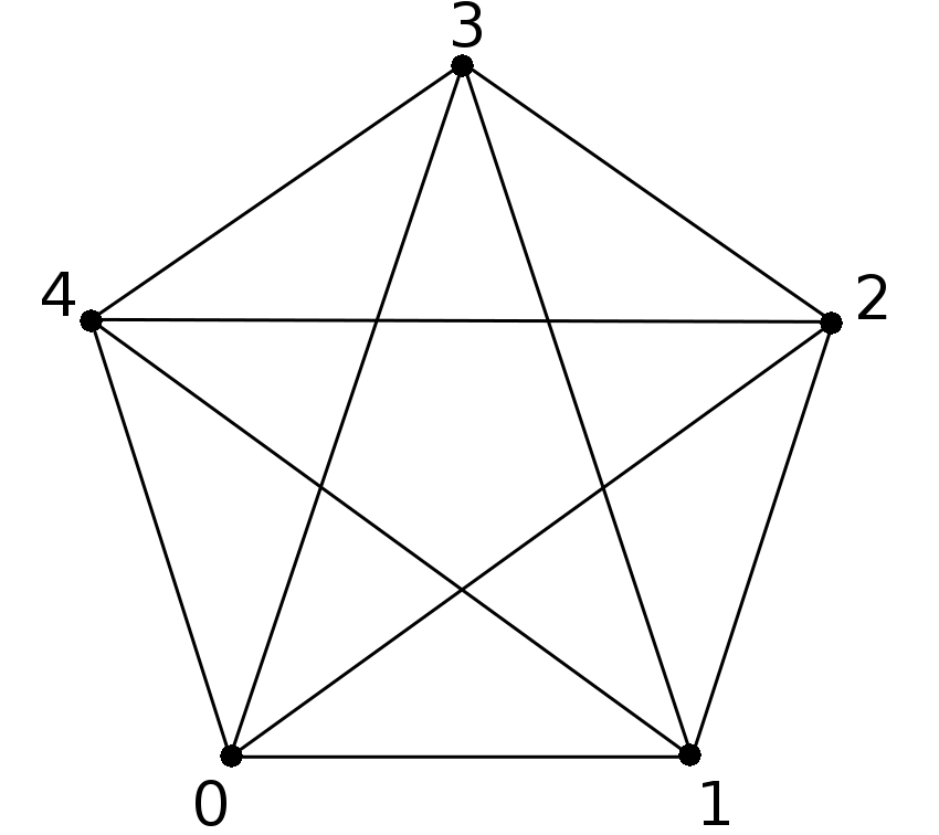
Figure 1: Complete graph on five nodes 0,…,40,\ldots,4.

In the standard EPRL-FK model [16, 17, 20] the vertex amplitude assigns a complex number to each SU(2) spin network s=(Γ,ȷ,ι)s=(\Gamma,\jmath,\iota). The asymptotic limit has been studied in the case when Γ\Gamma is a complete graph on five nodes 0,…,40,\ldots,4 (the unique graph connecting each pair of nodes with precisely one link) [35]. This means that spin networks with nodes labelled by the Livine-Speziale coherent intertwiners [38] were considered and the asymptotic limit when the spins ȷ\jmath (all different than 00) are uniformly rescaled by a large parameter Λ\Lambda was studied. The technical tool used in the calculation is an extended stationary phase method [50]. The amplitude can be written in the following form (see Section 2.7):

A⁡(s)=c​∫SL⁡(2,ℂ)5∏id​gi​δ​(g5)​∫(ℂ​ℙ1×ℂ​ℙ1)10(∏i<jMi​j)​eS⁡(gi,𝐳i​j),A(s)=c\int_{\SSL(2,{\mathbb{C}})^{5}}\prod_{i}dg_{i}\delta(g_{5})\int_{(\mathbb{CP}^{1}\times\mathbb{CP}^{1})^{10}}\left(\prod_{i<j}M_{ij}\right)e^{S(g_{i},\mathbf{z}_{ij})}, (2)

where Mi​jM_{ij} is a measure on (ℂ​ℙ1×ℂ​ℙ1)10(\mathbb{CP}^{1}\times\mathbb{CP}^{1})^{10} parametrized by spinors 𝐳i​j,𝐳j​i∈ℂ2\{0}\mathbf{z}_{ij},\mathbf{z}_{ji}\in\mathbb{C}^{2}\backslash\{0\}, which is invariant under the scaling ȷi​j↦Λ​ȷi​j\jmath_{ij}\mapsto\Lambda\jmath_{ij}, cc is a factor that scales approximately as c↦c​Λ20c\mapsto c\Lambda^{20} for large Λ\Lambda and S⁡(gi,zi​j)S(g_{i},z_{ij}) scales as S⁡(gi,zi​j)↦Λ​S​(gi,zi​j)S(g_{i},z_{ij})\mapsto\Lambda S(g_{i},z_{ij}). The number of critical points depends on the (coherent) spin-network ss.

Let us notice that inside the definition of a coherent state some arbitrary phase is hidden, so the total result will be influenced by an arbitrary phase that scales uniformly with the scaling of the labels. In the analysis of [35, 51] this phase was fixed. However the phase choice was done in a global way by considering the whole graph – not locally by choosing the phases separately for each node. This convention is useful only in considering vertices separately as the phases would be chosen differently for the same nodes glued to two different vertices (see however [41, 52, 42, 53])33 3 The sum of phases for 4-simplices glued together has a physical meaning.. The choice of the phase also leads to additional phase terms in the action of [35] (π\pi from thin wedges see Section 6.2 of [35]) that can be removed by a more judicious choice of overall coherent state phase. For these reasons we prefer to keep the phase unspecified. This leads to an additional arbitrary overall phase in the asymptotic limit. As a result we do not study the phase of each oscillatory term but a difference of phases between different terms.

In the original formulation of the EPRL model only tetrahedra that are spacelike were considered. As a result ss is an SU⁡(2)\SU(2) spin network. Our goal is to study the asymptotics of the EPRL-FK vertex amplitude generalized to include tetrahedra that are timelike [32, 54]. We limit to the subcase where the faces are of signature −⁣−--. As a result [32] we will restrict to discrete series of the SU⁡(1,1)\SU(1,1) representations that are labelled with spins ȷ\jmath44 4 In the other subcase of faces of signature +⁣−+- (see [32] for explanation of semiclassical origin of the notion) continuous series of SU(1,1) representations are used. We expect that that there may be some non-geometric critical points in the +⁣−+- case and therefore we leave it for further research (see 1.2 for a comment).. We will consider a generalization of SU⁡(2)\SU(2) spin networks, where the links are labelled with spins ȷ\jmath55 5 In fact by representations (ȷ,ρ)(\jmath,\rho) of SL⁡(2,ℂ)\SSL(2,{\mathbb{C}}) satisfying simplicity constraint, that is in our case ρ=2​γ​ȷ\rho=2\gamma\jmath. but the nodes are labelled either with SU⁡(2)\SU(2) intertwiners or SU⁡(1,1)\SU(1,1) intertwiners. In this paper we determine the critical points of the action SS for the generalized vertex amplitude written in the form (2). This is a crucial step for determination of the asymptotic behaviour of the vertex amplitude.

To each coherent state we will associate vectors vi​j∈M4v_{ij}\in M^{4} in Minkowski spacetime (see section 5.2.1) perpendicular to the standard normal Nic​a​nN_{i}^{can} (e0=(1,0,0,0)Te_{0}=(1,0,0,0)^{T} or e3=(0,0,0,1)Te_{3}=(0,0,0,1)^{T} depending on the type of embedding) such that bivectors ∗(vi​j∧Nic​a​n){\ast}(v_{ij}\wedge N_{i}^{can}) are spacelike. We will call them the boundary data. Following [35] we will say that (see 5.2.1)

  • •

    they satisfy closure condition if ∑jvi​j=0\sum_{j}v_{ij}=0,

  • •

    they are non-degenerate if for every node ii every 33 out of 44 vectors vi​jv_{ij} are independent.

With such vectors for each ii we can build, by the Minkowski theorem, [55, 56, 57] (for simplices in arbitrary signature, see section 6.3) a tetrahedron in Nic​a​n⟂N_{i}^{can\perp}, the faces of which have signature −⁣−--. The type of normal determines type of tetrahedra. For timelike normal e0e_{0} we have spacelike tetrahedra, for spacelike normal e3e_{3}, timelike (in fact mixed signature) tetrahedra. We can determine lengths of the edges of each tetrahedron ii.

Refer to caption
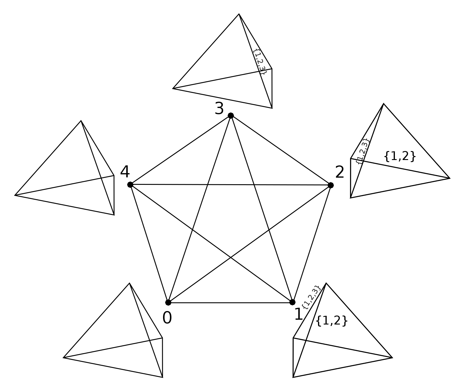
Figure 2: We consider a 44-simplex dual to the graph from figure 1. The nodes of the graph label tetrahedra of the simplex, links (sets of two nodes) label faces, edges between faces are labeled by sets of three nodes.

Let us consider a topological 44-simplex, the dual to the graph. The nodes of the graph label tetrahedra of the simplex, links (sets of two nodes) label faces, edges between faces are labeled by sets of three nodes (see figure 2. These nodes correspond to three tetrahedra sharing the edge. With every edge we can associate a length coming from application of Minkowski theorem to the boundary data in any node in the set. We will say that the lengths matching condition (definition 9) is satisfied if these lengths determined from all three tetrahedra are the same.

If the lengths matching condition is satisfied then we can look for the Gram matrix constructed from such lengths (see section 6.7). We can reconstruct a unique (up to reflections, rotations and shifts) 44 simplex from the Gram matrix. There are 55 cases for the signature of these simplices

  • •

    Lorentzian (+−−−+---),

  • •

    Euclidean (−−−−----),

  • •

    split signature (++−−++--),

  • •

    degenerate (+−−+--),

  • •

    degenerate (−−−---).

By the Minkowski theorem (for simplices in arbitrary signature, see section 6.3) we can also determine orientations of the reconstructed tetrahedra. If they match the orientations of tetrahedra of one of the reconstructed 44-simplices, we will say that orientations matching condition is satisfied (see Section 6.7 definition 10 for precise statement).

Our main result is summarized by the following theorem (see also the diagram on figure 1):

Closure condition?No critical pointsNoBoundary datanon-degenerate?Not addressedin Theorem 1NoLength matching?Orientation matching?Reconstructed 44-simplexnon-degenerate?22 critical pointsYes11 critical pointNoYesNo criticalpointsNoYesAt most 11critical pointNoYesYes
Figure 3: Classification of the critical points of the action SS according to Theorem 1.
Theorem 1.

If the boundary data vi​jv_{ij} does not satisfy the closure condition, the action has no critical point. Let us assume that the boundary data satisfies the closure condition and is non-degenerate. If the lengths matching condition is not satisfied then there exists at most one critical point of the action SS with the interpretation of a vector geometry [35]. The vector geometry can occur only if all normals are of the same type. If the lengths matching condition is satisfied but orientations matching condition is not, then the action has no critical points. If both conditions are satisfied, then let us consider the reconstructed 44-simplex Δ\Delta for the boundary data:

  • •

    If the reconstructed 44-simplex Δ\Delta is Lorentzian then there exist two critical points (gi,zi​j)(g_{i},z_{ij}) and (g~i,z~i​j)(\tilde{g}_{i},\tilde{z}_{ij}). The difference

    Δ​S=S⁡(gi,zi​j)−S⁡(g~i,z~i​j)\Delta S=S(g_{i},z_{ij})-S(\tilde{g}_{i},\tilde{z}_{ij})

    is given by the Regge action SΔS_{\Delta} without cosmological constant (1) for the flat 44-simplex Δ\Delta

    Δ​S=2​i⁡r​SΔmod2​π​i,\Delta S=2\iu rS_{\Delta}\mod 2\pi\iu,

    where r=±1r=\pm 1 is the Plebański orientation (definition 8).

  • •

    If the reconstructed 44-simplex Δ\Delta is Euclidean or of split signature then there exist two critical points (gi,zi​j)(g_{i},z_{ij}) and (g~i,z~i​j)(\tilde{g}_{i},\tilde{z}_{ij}). The difference Δ​S\Delta S is given by the Regge action:

    Δ​S=2​i⁡rγ​SΔmod2​π​i,\Delta S=\frac{2\iu r}{\gamma}S_{\Delta}\mod 2\pi\iu,

    where γ\gamma is the Barbero-Immirzi parameter.

  • •

    If the reconstructed 44 simplex is degenerate then there exists a single critical point.

Cases of signature −−−−---- (and ++−−++-- respectively) can occur only if all Nic​a​nN_{i}^{can} are e0e_{0} (and e3e_{3} respectively). Degenerate cases can occur only if all normals are of the same type (either e0e_{0} or e3e_{3}).

The case when all Nic​a​nN_{i}^{can} are equal to e0e_{0} was proven before (standard EPRL [35, 58]) but the other cases are our new result. As one can see, the case with timelike tetrahedra is similar to the previously obtained case with spacelike tetrahedra. The main difference is that in addition to Euclidean and Lorentzian signature also split-signature case is present.

Let us notice at the end that in our convention faces of the tetrahedra have areas Ai​j=12​ρi​jA_{ij}=\frac{1}{2}\rho_{ij} instead of ȷi​j\jmath_{ij} in the convention of [35]. This is just a total rescaling of the action by the Barbero-Immirzi parameter γ\gamma. Our convention is compatible with LQG area operator spectrum [59, 60]66 6 In LQG the area of the face would be Ai​j=8​π​G​ℏ​12​ρi​jA_{ij}=8\pi G\hbar\ \frac{1}{2}\rho_{ij} that would lead to the action 18​π​G​ℏ​SΔ\frac{1}{8\pi G\hbar}S_{\Delta}. We are using units 8​π​G​ℏ=18\pi G\hbar=1..

1.2 Type of faces

As we mentioned earlier, our analysis is restricted to the case when all faces are of signature (−−)(--) that is when the diagonal simplicity conditions of EPRL are [32]:

ρ=2​γ​ȷ.\rho=2\gamma\jmath. (3)

In the case of signature (−+)(-+) the simplicity constraint is:

2​ȷ=γ​ρ.2\jmath=\gamma\rho. (4)

This case is more complicated. Firstly, no EPRL like construction is known (see [48] for recent developments). Secondly, the coherent state proposition [32] in the line of Freidel-Krasnov model differs from representation theoretic construction in the style of EPRL. We expect that the asymptotic analysis in this case may lead to some unphysical sectors due to non-extremality of the necessary embeddings77 7 This problem is probably absent in Barrett-Crane model [12]..

We will give heuristic explanation of this fact. With the use of normal NN we can identify bivector BB in Minkowski spacetime M4M^{4} with two vectors L→,K→\vec{L},\vec{K} perpendicular to NN by formula

B=∗(N∧L→)+N∧K→.B=\ast(N\wedge\vec{L})+N\wedge\vec{K}. (5)

Regarding bivectors as generators of SO⁡(1,3)\SO(1,3) group we can write classical version of EPRL constraints imposed on the embedding. After some rearrangements we obtain:

L→⋅(L→+γ​K→)=0,(L→+γ​K→)2=0.\vec{L}\cdot(\vec{L}+\gamma\vec{K})=0,\quad(\vec{L}+\gamma\vec{K})^{2}=0. (6)

These are quadratic constraints whereas simplicity would be:

L→+γ​K→=0.\vec{L}+\gamma\vec{K}=0. (7)

Let us now describe case by case if from (6) follows (7).

  • •

    In the standard EPRL case: NN is timelike so L→\vec{L} and K→\vec{K} are spacelike so from (6) simplicity follows trivially as the only spacelike vector with norm zero is the zero vector.

  • •

    In the extended EPRL case with spacelike face: NN is spacelike but L→\vec{L} is timelike. From (6) we know that L→+γ​K→\vec{L}+\gamma\vec{K} is null. But there is no nontrivial null vector that is perpendicular to a nontrivial timelike vector, so L→+γ​K→=0\vec{L}+\gamma\vec{K}=0.

  • •

    In the extended EPRL case with timelike face: NN is spacelike and L→\vec{L} is spacelike. In this situation it might happen that L→+γ​K→≠0\vec{L}+\gamma\vec{K}\not=0 (simplicity fails).

As the simplicity (7) is crucial for the reconstruction of 44 simplex we suspect that there might be some non-geometric configurations for timelike faces.

1.3 Asymptotic analysis (conjecture)

The vertex amplitude is given by an oscillatory integral over an infinite domain. We would like to apply version of stationary phase analysis as presented for example in [50]. However in order to give a proper asymptotic result several technical conditions need to be satisfied.

  1. 1.

    finiteness. It is not known whether the evaluation of a spin network in the extended EPRL model is, in fact, finite. It was proven, but only for the standard EPRL setting (with all tetrahedra spacelike), that the integral defining the amplitude is absolutely convergent [61, 62]. The condition (well-definiteness of the definition) is necessary for any statement about the amplitude to make sense.

  2. 2.

    lack of boundary contributions. As the integral is over infinite domain with boundaries (or equivalently using compactification over domain with boundary) there might be some additional contributions to asymptotic expansion given by a version of Watson lemma. This is true as well in standard EPRL case (as the integration is over infinite domain), however in the extended set-up boundary is much more complicated. Preliminary check in the simpler Barrett-Crane model suggests that such contributions in fact appear but only for special boundary configurations that correspond to null (degenerate tetrahedra)88 8 In Barrett-Crane model only areas are specified but boundary contribution corresponds to a geometry of 4 simplex with null tetrahedra. In extended EPRL set-up one has additionally finite boundary of integrations. The integral at this boundary decays fast unless the spin of suitable representation is zero (degenerate or null face). This suggests that boundary contributions are related to null structures and we make the following conjecture: For nondegenerate boundary data (that excludes null faces and tetrahedra) there are no contributions from the boundary of integration. This issue was not addressed in any asymptotic analysis of the Lorentzian spin foam models so far. It is not a problem for the Euclidean models, as there is no boundary of the integration.

  3. 3.

    critical point non-degeneracy condition. An additional assumption is that, after suitably taking into account the symmetry of the action, the remaining matrix of second derivatives (Hessian) at the critical point is non-degenerate. This condition was never addressed in full generality in the analysis of the vertex amplitude. It was only checked for specific configurations in the standard EPRL model [35]. It is known that for the Barrett-Crane [12] spin foam models there are special configurations for which Hessian is degenerate [63]. However, this is probably related to the fact that the proper variables used in semiclassical description of this model are areas and conjugated angles [64, 65, 66] and there is some singularity in going from these variables to shapes. We conjecture that the Hessian is non-degenerate for the EPRL spin foam model for non-degenerate boundary data if the reconstructed 44 simplex is non-degenerate. The Hessian determinant is important for the asymptotic analysis as it determines asymptotic measure factor in the spin foam path integral. However, it is notoriously difficult to compute in terms of geometric quantities. The only known result for generic case is for the Barrett-Crane model [63]. If non-degeneracy fails, the scaling behaviour is different.

These issues definitely deserve a separate treatment and we leave them for future research. Under these conditions our results would give a proper asymptotic expansion of the extended EPRL vertex amplitude (see [50] and for the form of asymptotic vertex amplitude [35]).

1.4 Outline of the proof

In this paper we decided to give basically complete and detailed proof of the result. There are several reasons for that. First of all many of the subtle details of the classification of solutions are scattered in the literature and it is not easy to determined state of the affair. It is hard to find proof (extending to general case i.e. not using special properties of SU⁡(2)\SU(2)) that there are at most two critical points or that there are no critical points if orientations matching condition is not satisfied. Moreover, the extended EPRL model has more complicated geometry than the standard one. For example relation between two different critical points is more complicated than in standard case (they are not merely related by conjugation).

Because of that our paper is painfully long so for convenience of the reader we provide here an outline of the proof. We decided to work directly with the integral of EPRL YY-maps contracted using invariant bilinear form β\beta. It is in contrast to approach of [35] where β\beta integrals over (ℂ​ℙ1×ℂ​ℙ1)10(\mathbb{CP}^{1}\times\mathbb{CP}^{1})^{10} are perform analytically and a critical point is described by SL⁡(2,ℂ)\SSL(2,{\mathbb{C}}) group elements gig_{i}. The reason is that in extended case there are many subcases and the result would lead to higher complexity of the problem. This however means that there are more variables and our critical points are characterized by SL⁡(2,ℂ)\SSL(2,{\mathbb{C}}) group elements gig_{i} and and in addition spinors 𝐳i​j\mathbf{z}_{ij}.

First task is to write all the cases in the unified manner allowing to treat them at once. This is done in Section 2 and Section 3. After achieving this we concentrate on describing critical point conditions. In order to do this we need to derive certain properties of the action Section 4 (detailed exposition in appendix D). Critical points are written in terms of group and spinor variables. We can then use traceless matrices instead of spinors (proved in Section 4) obtaining what we call SL⁡(2,ℂ)\SSL(2,{\mathbb{C}}) solution. Up to additional information of spin lifts this are equivalent to geometric SO⁡(1,3)\SO(1,3) solution introduced in Section 5. The latter consists of a bunch of SO⁡(1,3)\SO(1,3) group elements that transform given boundary face bivectors such that they fit together.

As we know from standard EPRL asymptotic analysis two degenerate critical points can correspond to one geometric solution but in different signature. In order to incorporate this we develop theory of geometric solutions in arbitrary signature in Section 6. We show relation of the 44 simplex to geometric solutions (classifications in terms of reconstructed 44 simplices) in general. We have now direct correspondence between critical points and 44 simplices. In Section 7 we show how to construct 44 simplex of different signature from two degenerate critical points (vector geometries) in SO⁡(1,3)\SO(1,3) signature. In order to finish the proof we need classification that there are only two nondegenerate SO⁡(1,3)\SO(1,3), two vector geometries or single critical point. This is done in Section 8 together with the proof that if lengths matching condition is satisfied, but not the orientations matching condition then there is no critical point.

Parallelly to geometric description we compute difference of the phases between two critical points. As in the case of critical point description we lift the computation from original spinor description into the SO⁡(1,3)\SO(1,3) geometric description (or other signature computation). The problem with this approach is that in this way we loose some finite ambiguity of multiple of π\pi that need to be regained by the topological deformation argument. Most of the phase computation is done in Section 9.

2 Vertex amplitude in extended EPRL model

In this section we will describe extended EPRL embeddings [16, 32] and the construction of the vertex amplitude for a simplicial graph Γ\Gamma that was described in the introduction. The vertex amplitude in the spin foam models [67, 68, 21] is the evaluation of a certain spin network. This spin network consists of links labelled by irreducible unitary representations of SL⁡(2,ℂ)\SSL(2,{\mathbb{C}}) and nodes labelled by invariants in the tensor product of representations from links meeting in the node. These invariants are elements of a certain distribution space. Naïve evaluation would be the contraction of invariants according to the prescription given by the spin network. This prescription, while valid for a compact group, gives infinity for SL⁡(2,ℂ)\SSL(2,{\mathbb{C}}) and some gauge fixing [69, 61, 12] is necessary (see 2.7).

The spin network we consider is defined on a graph with five nodes 0,…,40,\ldots,4 connecting every node to every other one with precisely one link. We parametrize links by the two nodes (i​j)(ij) that they connect. The invariants at the nodes are given by group averaging the EPRL Y-maps (see section 2.4),

Inv⁡⨂l∋nSt⁡(Nnc​a​n)⁡ℋE​P​R​L​(ȷ,ρ)\displaystyle\Inv_{\St(N^{can}_{n})}\bigotimes_{l\ni n}{\mathcal{H}}_{EPRL(\jmath,\rho)} →Inv⁡⨂l∋nSL⁡(2,ℂ)⁡Dȷl,ρl\displaystyle\rightarrow\Inv_{\SSL(2,{\mathbb{C}})}\bigotimes_{l\ni n}D_{\jmath_{l},\rho_{l}} (8)
ψ\displaystyle\psi →∫SL⁡(2,ℂ)/St⁡(Nnc​a​n)d⁡[g]​g​ψ,\displaystyle\rightarrow\int_{\SSL(2,{\mathbb{C}})/\St(N^{can}_{n})}d[g]\ g\psi, (9)

where the group St⁡(Nnc​a​n)⊂SL⁡(2,ℂ)\St(N^{can}_{n})\subset\SSL(2,{\mathbb{C}}) is a subgroup stabilizing the normal Nnc​a​nN^{can}_{n}, ll are links meeting in the node nn and ℋE​P​R​L​(ȷ,ρ){\mathcal{H}}_{EPRL(\jmath,\rho)} is certain representation of St⁡(Nnc​a​n)\St(N^{can}_{n}). Invariants of the subgroup St⁡(Nnc​a​n)\St(N^{can}_{n}) are thus together with labels and type of the subgroup (determined by Nnc​a​nN^{can}_{n}) the boundary data for the vertex amplitude.

We are interested in the asymptotic analysis for large labels. In such a case one needs to specify a family of boundary states with certain semiclassical limit. Examples of such states are given by coherent states (they scale nicely with the scaling of labels) integrated over the subgroup:

ψ=∫St⁡(Nnc​a​n)dgg(⊗l∋nΨl).\psi=\int_{\St(N^{can}_{n})}dg\ g\left(\otimes_{l\ni n}\Psi_{l}\right). (10)

We will now describe in unified manner the choice of coherent states and their image under the Y-map. We will present also the form of the vertex amplitude (using bilinear forms β\beta used to contract invariants [35]).

2.1 Notation

Let us summarize notation about spinors and SL⁡(2,ℂ)→SO+⁡(1,3)\SSL(2,{\mathbb{C}})\rightarrow\SO_{+}(1,3) double cover. We use signature +−−−+---.

Let us introduce σμ\sigma_{\mu} as follows

σ0=𝕀,σi​ Pauli matrices\sigma_{0}={\mathbb{I}},\ \sigma_{i}\text{ Pauli matrices} (11)

We have the following isomorphism from Minkowski space M4M^{4} into Hermitian 2×22\times 2 matrices

M4∋Nμ→ηN=Nμ​σμ​ with ​Nμ​Nμ=detηNM^{4}\ni N^{\mu}\rightarrow\eta_{N}=N^{\mu}\sigma_{\mu}\text{ with }N_{\mu}N^{\mu}=\det\eta_{N} (12)

The symplectic form is defined as

ω=(01−10),ω¯=ω,ω−1=ωT=−ω,\omega=\left(\begin{array}[]{cc}0&1\\ -1&0\end{array}\right),\quad\bar{\omega}=\omega,\ \omega^{-1}=\omega^{T}=-\omega, (13)

We will also use a notation for two spinors 𝐳\mathbf{z} and 𝐰\mathbf{w}

[𝐳,𝐰]=𝐳T​ω​w=z0​w1−z1​w0,𝐳=(z0z1),𝐰=(w0w1)[\mathbf{z},\mathbf{w}]=\mathbf{z}^{T}\omega\textbf{w}=z_{0}w_{1}-z_{1}w_{0},\quad\mathbf{z}=\left(\begin{array}[]{c}{z_{0}}\\ {z_{1}}\end{array}\right),\quad\mathbf{w}=\left(\begin{array}[]{c}{w_{0}}\\ {w_{1}}\end{array}\right) (14)

Let us also introduce

σ^μ=−ω​σμT​ω={σ0μ=0−σiμ=i,η^N=Nμ​σ^μ​ Hermitian\hat{\sigma}_{\mu}=-\omega\sigma_{\mu}^{T}\omega=\left\{\begin{array}[]{ll}\sigma_{0}&\mu=0\\ -\sigma_{i}&\mu=i\end{array}\right.,\quad\hat{\eta}_{N}=N^{\mu}\hat{\sigma}_{\mu}\text{ Hermitian} (15)

The following holds

σν​σ^μ+σμ​σ^ν=2​gμ​ν​𝕀\displaystyle\sigma_{\nu}\hat{\sigma}_{\mu}+\sigma_{\mu}\hat{\sigma}_{\nu}=2g_{\mu\nu}{\mathbb{I}} (16)
σ^ν​σμ+σ^μ​σν=2​gμ​ν​𝕀\displaystyle\hat{\sigma}_{\nu}\sigma_{\mu}+\hat{\sigma}_{\mu}\sigma_{\nu}=2g_{\mu\nu}{\mathbb{I}} (17)

Together σμ\sigma_{\mu} and σ^μ\hat{\sigma}_{\mu} form γμ\gamma_{\mu} matrix, but as we always work in either self-dual or anti-self-dual representation we prefer such a notation.

From standard commutation relation we have

Nμ​Mμ=12​tr⁡ηN​η^M,N^{\mu}M_{\mu}=\frac{1}{2}\tr\eta_{N}\hat{\eta}_{M}, (18)

The isomorphism π\pi from SL⁡(2,ℂ)\SSL(2,{\mathbb{C}}) to SO+⁡(1,3)\SO_{+}(1,3) is defined by

π⁡(u)​(N)μ​σμ=u⁡(Nμ​σμ)​u†\pi(u)(N)^{\mu}\sigma_{\mu}=u\ (N^{\mu}\sigma_{\mu})\ u^{\dagger} (19)

Lie algebra of SO+⁡(1,3)\SO_{+}(1,3) can be identify with bivectors (22 forms). The action of bivectors on vectors is defined by contraction with the use of the metric

B⁡(v)=B​⌟​vB(v)=B\lrcorner v (20)

The identification of s​o​(1,3)so(1,3) with s​l​(2,ℂ)sl(2,{\mathbb{C}}) is then given on the basic simple bivectors by

s​o​(1,3)∋B=a∧b⟶𝔹=14​(ηa​η^b−ηb​η^a)∈s​l​(2,ℂ)so(1,3)\ni B=a\wedge b\longrightarrow{\mathbb{B}}=\frac{1}{4}(\eta_{a}\hat{\eta}_{b}-\eta_{b}\hat{\eta}_{a})\in sl(2,{\mathbb{C}}) (21)

With the right choice of the orientation the Hodge ∗{\ast} operation corresponds to multiplication by ii of the traceless matrix.

2.2 Representations of SL⁡(2,ℂ)\SSL(2,{\mathbb{C}})

Unitary irreducible representations (Dȷ,ρD_{\jmath,\rho}) from the principal series (ȷ,ρ)(\jmath,\rho) are functions

ℂ2∖{0}∋𝐳→Ψ(𝐳)∈ℂ,,𝐳=(z0z1){\mathbb{C}}^{2}\setminus\{0\}\ni\mathbf{z}\rightarrow\Psi(\mathbf{z})\in{\mathbb{C}},\quad,\quad\mathbf{z}=\left(\begin{array}[]{c}{z_{0}}\\ {z_{1}}\end{array}\right) (22)

satisfying the condition

Ψ⁡(ei​ϕ+r​𝐳)=ei⁡(2​ȷ​ϕ+ρ​r)−2​r​Ψ​(𝐳),\Psi(e^{i\phi+r}\mathbf{z})=e^{i(2\jmath\phi+\rho r)-2r}\Psi(\mathbf{z}),\quad (23)

with the action of SL⁡(2,ℂ)\SSL(2,{\mathbb{C}}) defined by

g​Ψ​(𝐳)=Ψ⁡(gT​𝐳)g\Psi(\mathbf{z})=\Psi(g^{T}\mathbf{z}) (24)

We are using the convention of [35], as opposed to that of [70]. The latter is equivalent to the action

g​Ψ​(𝐳)=Ψ⁡(g−1​𝐳)g\Psi(\mathbf{z})=\Psi(g^{-1}\mathbf{z}) (25)

These two actions can be related due to

g−1=ω−1​gT​ωg^{-1}=\omega^{-1}g^{T}\omega (26)

The scalar product for two such functions Ψ1\Psi_{1} and Ψ2\Psi_{2} is defined as follows: Let us introduce a form

Ψ1​(𝐳)¯​Ψ2​(𝐳)​Ω𝐳\overline{\Psi_{1}(\mathbf{z})}\Psi_{2}(\mathbf{z})\Omega_{\mathbf{z}} (27)

where

Ω𝐳:=i2​(z0​d​z1−z1​d​z0)∧(z0¯​d​z¯1−z¯1​d​z¯0),𝐳=(z0z1)\Omega_{\mathbf{z}}:=\frac{\iu}{2}\left(z_{0}dz_{1}-z_{1}dz_{0}\right)\wedge\left(\overline{z_{0}}d\overline{z}_{1}-\overline{z}_{1}d\overline{z}_{0}\right),\quad\mathbf{z}=\left(\begin{array}[]{c}{z_{0}}\\ {z_{1}}\end{array}\right) (28)

The form (27) is invariant under the scaling transformation

𝐳→λ​𝐳,λ∈ℂ∗\mathbf{z}\rightarrow\lambda\mathbf{z},\quad\lambda\in{\mathbb{C}}^{*} (29)

and is annihilated by the generator of this transformation, thus it descends to a form on ℂ​ℙ1\mathbb{CP}^{1}

⟨Ψ1,Ψ2⟩=∫ℂ​ℙ1Ψ1​(𝐳)¯​Ψ2​(𝐳)​Ω𝐳\langle\Psi_{1},\Psi_{2}\rangle=\int_{\mathbb{CP}^{1}}\overline{\Psi_{1}(\mathbf{z})}\Psi_{2}(\mathbf{z})\Omega_{\mathbf{z}} (30)

2.3 Subgroups preserving the normal NN

The subgroup of SO+⁡(1,3)\SO_{+}(1,3) that preserves the normal NN is the image of the subgroup of SL⁡(2,ℂ)\SSL(2,{\mathbb{C}}) that preserves ηN\eta_{N} as follows

St⁡(N)={g∈SL⁡(2,ℂ):π⁡(g)​N=N}={g∈SL⁡(2,ℂ):g​ηN​g†=ηN}\St(N)=\{g\in\SSL(2,{\mathbb{C}})\colon\pi(g)N=N\}=\{g\in\SSL(2,{\mathbb{C}})\colon g\eta_{N}g^{\dagger}=\eta_{N}\} (31)

this is equivalent to gTg^{T} preserving Hermitian form defined by

⟨𝐳1,𝐳2⟩N=𝐳1†​ηNT​𝐳2=𝐳2T​ηN​𝐳1¯\langle\mathbf{z}_{1},\mathbf{z}_{2}\rangle_{N}=\mathbf{z}_{1}^{\dagger}\eta_{N}^{T}\mathbf{z}_{2}=\mathbf{z}_{2}^{T}\eta_{N}\overline{\mathbf{z}_{1}} (32)

It follows from the fact that

⟨gT​𝐳1,gT​𝐳2⟩N=𝐳2T​g​ηN​g¯T⏟=ηN​𝐳1¯=⟨𝐳1,𝐳2⟩N\langle g^{T}\mathbf{z}_{1},g^{T}\mathbf{z}_{2}\rangle_{N}=\mathbf{z}_{2}^{T}\underbrace{g\eta_{N}\bar{g}^{T}}_{=\eta_{N}}\overline{\mathbf{z}_{1}}=\langle\mathbf{z}_{1},\mathbf{z}_{2}\rangle_{N} (33)

for g∈St⁡(N)g\in\St(N).

2.4 The Y map

Let us review the generalized EPRL construction. As explained in the introduction, we will work only with spacelike surfaces. Let us consider a normal vector NN

Nμ​Nμ=t,t∈{−1,1}N_{\mu}N^{\mu}=t,\quad t\in\{-1,1\} (34)

where t=1t=1 for timelike, t=−1t=-1 for spacelike vector. Let us consider stabilizing group St⁡(N)\St(N). In the case of t=1t=1,

St⁡(N)≅SU⁡(2)\St(N)\cong\SU(2) (35)

and it is exactly SU⁡(2)\SU(2) for N=e0=(1,0,0,0)N=e_{0}=(1,0,0,0). For t=−1t=-1

St⁡(N)≅SU⁡(1,1)\St(N)\cong\SU(1,1) (36)

and it is exactly SU⁡(1,1)\SU(1,1) for N=e3=(0,0,0,1)N=e_{3}=(0,0,0,1).

We will consider only standard normals e0=(1,0,0,0)e_{0}=(1,0,0,0) and e3=(0,0,0,1)e_{3}=(0,0,0,1). We will also denote either of them by NcanN^{\text{can}} as we would like to work in a unified setup. We denote tc​a​n=Nc​a​n⋅Nc​a​nt^{can}=N^{can}\cdot N^{can}.

The EPRL YY map is an embedding of the unitary representation of the stabilizing group St⁡(N)\St(N) into unitary representation (ȷ,ρ=2​γ​ȷ)(\jmath,\rho=2\gamma\jmath) of SL⁡(2,ℂ)\SSL(2,{\mathbb{C}}) that satisfies a certain extremality condition. Let us recall the choice of ℋE​P​R​L​(ȷ,ρ){\mathcal{H}}_{EPRL(\jmath,\rho)} made by [16, 32]

  1. 1.

    Spin ȷ\jmath, DȷD_{\jmath} representation of SU⁡(2)\SU(2) embedded into Dȷ,ρD_{\jmath,\rho} for Nc​a​n=e0N^{can}=e_{0}

  2. 2.

    Discrete series Dȷ±D_{\jmath}^{\pm} of spin ȷ\jmath representations of SU⁡(1,1)\SU(1,1) embedded into Dȷ,ρD_{\jmath,\rho} for Nc​a​n=e3N^{can}=e_{3}

2.5 Coherent states

All three families of representations have certain common features. Let us consider the generator of rotations around the zz axis. We can introduce bases of eigenfunctions. In all three cases there exists an extreme eigenvalue. The corresponding eigenfunctions are (Perelomov-)coherent states [71, 49, 70] (see Appendix C)99 9 We do not need to consider −ȷ-\jmath for SU⁡(2)\SU(2) since it will be obtained from ȷ\jmath eigenstate by rotation.

  • •

    For Nc​a​n=e0N^{can}=e_{0}

    Fȷ​ȷ​(𝐳)=2​ȷ+12​π​⟨𝐳|𝐳⟩Nc​a​ni⁡ρ2−1−ȷ​⟨𝐧0|𝐳⟩Nc​a​n2​ȷ,F_{\jmath\jmath}(\mathbf{z})=\sqrt{\frac{2\jmath+1}{2\pi}}\left<\mathbf{z}|\mathbf{z}\right>_{N^{can}}^{\iu\frac{\rho}{2}-1-\jmath}\left<\mathbf{n}_{0}|\mathbf{z}\right>_{N^{can}}^{2\jmath}, (37)
  • •

    For Nc​a​n=e3N^{can}=e_{3}

    Fȷ​ȷ+​(𝐳)=2​ȷ−1π​θ​(⟨𝐳|𝐳⟩Nc​a​n)​⟨𝐳|𝐳⟩Nc​a​ni⁡ρ2−1+ȷ​⟨𝐳|𝐧0⟩Nc​a​n−2​ȷ,\displaystyle F^{+}_{\jmath\jmath}(\mathbf{z})=\sqrt{\frac{2\jmath-1}{\pi}}\theta(\left<\mathbf{z}|\mathbf{z}\right>_{N^{can}})\left<\mathbf{z}|\mathbf{z}\right>_{N^{can}}^{\iu\frac{\rho}{2}-1+\jmath}\left<\mathbf{z}|\mathbf{n}_{0}\right>_{N^{can}}^{-2\jmath}, (38)
    Fȷ−ȷ−​(𝐳)=2​ȷ−1π​θ​(−⟨𝐳|𝐳⟩Nc​a​n)​(−⟨𝐳|𝐳⟩Nc​a​n)i⁡ρ2−1+ȷ​(−⟨𝐳|𝐧1⟩Nc​a​n)−2​ȷ,\displaystyle F^{-}_{\jmath-\jmath}(\mathbf{z})=\sqrt{\frac{2\jmath-1}{\pi}}\theta(-\left<\mathbf{z}|\mathbf{z}\right>_{N^{can}})(-\left<\mathbf{z}|\mathbf{z}\right>_{N^{can}})^{\iu\frac{\rho}{2}-1+\jmath}(-\left<\mathbf{z}|\mathbf{n}_{1}\right>_{N^{can}})^{-2\jmath}, (39)

where 𝐧0=(1,0)\mathbf{n}_{0}=(1,0) and 𝐧1=(0,1)\mathbf{n}_{1}=(0,1) and θ\theta is the Heaviside step function.

All other coherent states are obtained by transforming these basic coherent states by group action of St⁡(Nc​a​n)\St(N^{can}). In fact these states can be parametrized by spinors:

Ψ𝐧​(𝐳)=2​ȷ+12​π​⟨𝐳|𝐳⟩Nc​a​ni⁡ρ2−1−ȷ​⟨𝐧|𝐳⟩Nc​a​n2​ȷ,⟨𝐧|𝐧⟩Nc​a​n=1,Nc​a​n=e0\Psi^{\mathbf{n}}(\mathbf{z})=\sqrt{\frac{2\jmath+1}{2\pi}}\left<\mathbf{z}|\mathbf{z}\right>_{N^{can}}^{\iu\frac{\rho}{2}-1-\jmath}\left<\mathbf{n}|\mathbf{z}\right>_{N^{can}}^{2\jmath},\quad\left<\mathbf{n}|\mathbf{n}\right>_{N}^{can}=1,\ N^{can}=e_{0} (40)

and for Nc​a​n=e3N^{can}=e_{3}

Ψ+,𝐧+​(𝐳)\displaystyle\Psi^{+,\mathbf{n}^{+}}(\mathbf{z}) =θ⁡(⟨𝐳|𝐳⟩Nc​a​n)​2​ȷ−1π​⟨𝐳|𝐳⟩Nc​a​ni⁡ρ2−1+ȷ​⟨𝐳|𝐧+⟩Nc​a​n−2​j\displaystyle=\theta(\left<\mathbf{z}|\mathbf{z}\right>_{N^{can}})\sqrt{\frac{2\jmath-1}{\pi}}\left<\mathbf{z}|\mathbf{z}\right>_{N^{can}}^{\iu\frac{\rho}{2}-1+\jmath}\left<\mathbf{z}|\mathbf{n}^{+}\right>^{-2j}_{N^{can}} (41)
Ψ−,𝐧−​(𝐳)\displaystyle\Psi^{-,\mathbf{n}^{-}}(\mathbf{z}) =θ⁡(−⟨𝐳|𝐳⟩Nc​a​n)​2​ȷ−1π​(−⟨𝐳|𝐳⟩Nc​a​n)i⁡ρ2−1+ȷ​(−⟨𝐳|𝐧−⟩Nc​a​n)−2​ȷ,\displaystyle=\theta(-\left<\mathbf{z}|\mathbf{z}\right>_{N^{can}})\sqrt{\frac{2\jmath-1}{\pi}}(-\left<\mathbf{z}|\mathbf{z}\right>_{N^{can}})^{\iu\frac{\rho}{2}-1+\jmath}(-\left<\mathbf{z}|\mathbf{n}^{-}\right>_{N^{can}})^{-2\jmath}, (42)

where ⟨𝐧±|𝐧±⟩Nc​a​n=±1\left<\mathbf{n}^{\pm}|\mathbf{n}^{\pm}\right>_{N^{can}}=\pm 1.

2.6 Bilinear invariant form

Let us recall the definition of the bilinear, SL⁡(2,ℂ)\SSL(2,{\mathbb{C}})-invariant form [72]

β⁡(Φ,Φ′):=\displaystyle\beta(\Phi,\Phi^{\prime}):= (ρ2)2+ȷ2π​∫ℂ​ℙ1×ℂ​ℙ1Ω𝐳∧Ω𝐳′​|[𝐳,𝐳′]|−2​[𝐳,𝐳′]−i⁡ρ2−ȷ​[𝐳,𝐳′]¯−i⁡ρ2+ȷ⏟β⁡(𝐳,𝐳′)\displaystyle\frac{\sqrt{\left(\frac{\rho}{2}\right)^{2}+\jmath^{2}}}{\pi}\int_{\mathbb{CP}^{1}\times\mathbb{CP}^{1}}\underbrace{\Omega_{\mathbf{z}}\wedge\Omega_{\mathbf{z}^{\prime}}|[\mathbf{z},\mathbf{z}^{\prime}]|^{-2}[\mathbf{z},\mathbf{z}^{\prime}]^{-\iu\frac{\rho}{2}-\jmath}{\overline{[\mathbf{z},\mathbf{z}^{\prime}]}}^{-\iu\frac{\rho}{2}+\jmath}}_{\beta(\mathbf{z},\mathbf{z}^{\prime})}
⋅Φ⁡(𝐳)​Φ′​(𝐳′)\displaystyle\cdot{}\Phi(\mathbf{z})\Phi^{\prime}(\mathbf{z}^{\prime}) (43)

where Φ,Φ′\Phi,\Phi^{\prime} are elements of the SL⁡(2,ℂ)\SSL(2,{\mathbb{C}})-representation (ȷ,ρ)(\jmath,\rho), and Ω𝐳\Omega_{\mathbf{z}} is defined in (28).

2.7 The vertex amplitude

We can now consider the vertex amplitude in the spin foam model. Let us consider the pentagonal graph [35] with five nodes and links connecting each node with each other.

  • •

    for every node ii we choose a canonical normal Nic​a​nN_{i}^{can} that determines an embedded subgroup (either SU⁡(2)\SU(2) or SU⁡(1,1)\SU(1,1))

  • •

    for every directed link i​jij starting in the node ii we chose a type of embedded representation (in case of SU⁡(1,1)\SU(1,1) it can be Dȷi​j+D_{\jmath_{ij}}^{+} or Dȷi​j−D_{\jmath_{ij}}^{-} and for SU⁡(2)\SU(2) it is Dȷi​jD_{\jmath_{ij}})

  • •

    for every directed link i​jij starting in the node ii we chose a spinor 𝐧i​j\mathbf{n}_{ij} that determines a coherent state (in representation (ȷi​j,ρi​j)(\jmath_{ij},\rho_{ij}) of SL⁡(2,ℂ)\SSL(2,{\mathbb{C}})) that we will denote by Ψi​j​(𝐳)\Psi_{ij}(\mathbf{z})

This data is a boundary data for the vertex amplitude of the extended EPRL Spin Foam model [35, 32].

The vertex amplitude is given by an integral

Av=∫SL⁡(2,ℂ)5∏id​gi​δ​(g5)​∏i<jβ⁡(gi​Ψi​j,gj​Ψj​i),A_{v}=\int_{\SSL(2,{\mathbb{C}})^{5}}\prod_{i}dg_{i}\delta(g_{5})\prod_{i<j}\beta(g_{i}\Psi_{ij},g_{j}\Psi_{ji}),

where

gi​Ψi​j​(𝐳)=Ψi​j​(giT​𝐳)g_{i}\Psi_{ij}(\mathbf{z})=\Psi_{ij}(g_{i}^{T}\mathbf{z})

and the δ⁡(g5)\delta(g_{5}) is a gauge fixing. We will denote 𝐳i​j\mathbf{z}_{ij} and 𝐳j​i\mathbf{z}_{ji} the variables 𝐳\mathbf{z} and 𝐳′\mathbf{z}^{\prime} in the β\beta integral for nodes i,ji,j.

3 Stationary phase approximation

In this section we will write the amplitude from section 2.7 in a form suitable for the stationary phase method. We will consider the uniform scaling of the representations (we remind that ρ\rho and ȷ\jmath are related by the simplicity constraint)

(ȷi​j,ρi​j)↦(Λ​ȷi​j,Λ​ρi​j),Λ∈ℕ+(\jmath_{ij},\rho_{ij})\mapsto(\Lambda\jmath_{ij},\Lambda\rho_{ij}),\quad\Lambda\in{\mathbb{N}}_{+}

and we want to organize the integral in the form c⁡(Λ)​∫f​eΛ​Sc(\Lambda)\int fe^{\Lambda S}. This will provide a definition of the action. The amplitude is written as integral of the product of many terms and we will focus on each term separately. The total action will be the sum of these partial contributions.

We will write conditions for the critical points of this action in terms of holomorphic derivatives, since that is the form that we will use later.

We will assume that (ȷi​j,ρi​j)≠0(\jmath_{ij},\rho_{ij})\not=0. Again, we expect that representations (ȷi​j,ρi​j)=(0,0)(\jmath_{ij},\rho_{ij})=(0,0) are of special interest. They should correspond to null surfaces.

3.1 Scaled amplitude

We denote the normal stabilized by the embedded group by Nic​a​nN_{i}^{can},

Nic​a​n⋅Nic​a​n=tic​a​n,⟨𝐧i​j,𝐧i​j⟩Nic​a​n=si​j,si​j,tic​a​n∈{−1,1}N_{i}^{can}\cdot N_{i}^{can}=t_{i}^{can},\quad\langle\mathbf{n}_{ij},\mathbf{n}_{ij}\rangle_{N_{i}^{can}}=s_{ij},\quad s_{ij},t_{i}^{can}\in\{-1,1\} (44)

The coherent states decompose under the scaling in the following way,

Ψi​jΛ​(𝐳i​j)=ci​j​(Λ)​mi​j​(𝐳)​pi​j​(𝐳i​j)Λ\Psi_{ij}^{\Lambda}(\mathbf{z}_{ij})=c_{ij}(\Lambda)m_{ij}(\mathbf{z})p_{ij}(\mathbf{z}_{ij})^{\Lambda}

where mi​j,pi​jm_{ij},p_{ij} independent of Λ\Lambda

mi​j​(𝐳i​j)=θ⁡(si​j​⟨𝐳i​j|𝐳i​j⟩Nic​a​n)​(si​j​⟨𝐳i​j|𝐳i​j⟩Nic​a​n)−1m_{ij}(\mathbf{z}_{ij})=\theta(s_{ij}\langle\mathbf{z}_{ij}|\mathbf{z}_{ij}\rangle_{N_{i}^{can}})(s_{ij}\langle\mathbf{z}_{ij}|\mathbf{z}_{ij}\rangle_{N_{i}^{can}})^{-1} (45)

with notice that for Nic​a​n=e0N^{can}_{i}=e_{0}, si​j​⟨𝐳i​j|𝐳i​j⟩Nic​a​n>0s_{ij}\langle\mathbf{z}_{ij}|\mathbf{z}_{ij}\rangle_{N_{i}^{can}}>0 on the whole ℂ2∖{0}{\mathbb{C}}^{2}\setminus\{0\}. Function pi​jp_{ij} is given explicitly (uniform description) by

pi​j=pi​jρ​pi​jȷp_{ij}=p_{ij}^{\rho}p_{ij}^{\jmath} (46)

where

pi​jρ=(si​j​⟨giT​𝐳i​j,giT​𝐳i​j⟩Nic​a​n)i​ρi​j2,pi​jȷ={pi​ja​u​x,tic​a​n=−1pi​ja​u​x¯,tic​a​n=1\displaystyle p_{ij}^{\rho}=\left(s_{ij}\langle g_{i}^{T}\mathbf{z}_{ij},g_{i}^{T}\mathbf{z}_{ij}\rangle_{N_{i}^{can}}\right)^{i\frac{\rho_{ij}}{2}},\quad p_{ij}^{\jmath}=\left\{\begin{array}[]{ll}p_{ij}^{aux},&t_{i}^{can}=-1\\ \overline{p_{ij}^{aux}},&t_{i}^{can}=1\end{array}\right.

with

pi​ja​u​x=(si​j​⟨giT​𝐳i​j,𝐧i​j⟩Nic​a​n(si​j​⟨giT​𝐳i​j,giT​𝐳i​j⟩Nic​a​n)1/2)tic​a​n​ 2​ȷi​jp_{ij}^{aux}=\left(\frac{s_{ij}\langle g_{i}^{T}\mathbf{z}_{ij},\mathbf{n}_{ij}\rangle_{N_{i}^{can}}}{(s_{ij}\langle g_{i}^{T}\mathbf{z}_{ij},g_{i}^{T}\mathbf{z}_{ij}\rangle_{N_{i}^{can}})^{1/2}}\right)^{t_{i}^{can}\ 2\jmath_{ij}} (49)

The factors ci​j​(Λ)c_{ij}(\Lambda) are independent from 𝐳\mathbf{z} and gg

ci​j​(Λ)={2​Λ​ȷi​j+12​π,Nic​a​n=e0​ and ​Dȷ​ representation2​Λ​ȷi​j−1π,Nic​a​n=e3​ and ​Dȷ±​ representationc_{ij}(\Lambda)=\left\{\begin{array}[]{ll}\sqrt{\frac{2\Lambda\jmath_{ij}+1}{2\pi}},&N_{i}^{can}=e_{0}\text{ and }D_{\jmath}\text{ representation}\\ \sqrt{\frac{2\Lambda\jmath_{ij}-1}{\pi}},&N_{i}^{can}=e_{3}\text{ and }D^{\pm}_{\jmath}\text{ representation}\end{array}\right. (50)

Similarly, we can decompose the integral kernel of β\beta as

βi​jΛ​(𝐳i​j,𝐳j​i)=ci​jβ​(Λ)​mi​jβ​(𝐳i​j,𝐳j​i)​pi​jβ​(𝐳i​j,𝐳j​i)Λ\beta_{ij}^{\Lambda}(\mathbf{z}_{ij},\mathbf{z}_{ji})=c_{ij}^{\beta}(\Lambda)m^{\beta}_{ij}(\mathbf{z}_{ij},\mathbf{z}_{ji})p^{\beta}_{ij}(\mathbf{z}_{ij},\mathbf{z}_{ji})^{\Lambda}

where ci​jβ​(Λ)=Λ​(ρi​j2)2+ȷi​j2πc_{ij}^{\beta}(\Lambda)=\Lambda\frac{\sqrt{\left(\frac{\rho_{ij}}{2}\right)^{2}+\jmath_{ij}^{2}}}{\pi},

mi​jβ​(𝐳i​j,𝐳j​i)\displaystyle m^{\beta}_{ij}(\mathbf{z}_{ij},\mathbf{z}_{ji}) =Ω𝐳i​j∧Ω𝐳j​i​|[𝐳i​j,𝐳j​i]|−2\displaystyle=\Omega_{\mathbf{z}_{ij}}\wedge\Omega_{\mathbf{z}_{ji}}|[\mathbf{z}_{ij},\mathbf{z}_{ji}]|^{-2} (51)
pi​jβ​(𝐳i​j,𝐳j​i)\displaystyle p^{\beta}_{ij}(\mathbf{z}_{ij},\mathbf{z}_{ji}) =[𝐳i​j,𝐳j​i]−i⁡ρi​j2−ȷi​j​[𝐳i​j,𝐳j​i]¯−i⁡ρi​j2+ȷi​j\displaystyle=[\mathbf{z}_{ij},\mathbf{z}_{ji}]^{-\iu\frac{\rho_{ij}}{2}-\jmath_{ij}}{\overline{[\mathbf{z}_{ij},\mathbf{z}_{ji}]}}^{-\iu\frac{\rho_{ij}}{2}+\jmath_{ij}} (52)

The differential form

Mi​j:=mi​jβ​(𝐳i​j,𝐳j​i)​mi​j​(giT​𝐳i​j)​mj​i​(gjT​𝐳j​i)M_{ij}:=m^{\beta}_{ij}(\mathbf{z}_{ij},\mathbf{z}_{ji})m_{ij}(g_{i}^{T}\mathbf{z}_{ij})m_{ji}(g_{j}^{T}\mathbf{z}_{ji})\qquad

descends to ℂ​ℙ1×ℂ​ℙ1\mathbb{CP}^{1}\times\mathbb{CP}^{1} as a measure (smooth in the interior of its support).

Similarly1010 10 The scaling invariance of Pi​jP_{ij} and descendent property of μi​j\mu_{ij} is a general fact., as the integrand form is invariant under rescaling of 𝐳\mathbf{z} also the part scaled uniformly with Λ\Lambda need to be invariant. The amplitude

Pi​j:=pi​jβ​(𝐳i​j,𝐳j​i)​pi​j​(giT​𝐳i​j)​pj​i​(gjT​𝐳j​i)P_{ij}:=p^{\beta}_{ij}(\mathbf{z}_{ij},\mathbf{z}_{ji})p_{ij}(g_{i}^{T}\mathbf{z}_{ij})p_{ji}(g_{j}^{T}\mathbf{z}_{ji})

is invariant under rescalings 𝐳i​j↦λi​j​𝐳i​j\mathbf{z}_{ij}\mapsto\lambda_{ij}\mathbf{z}_{ij}, 𝐳j​i↦λj​i​𝐳j​i\mathbf{z}_{ji}\mapsto\lambda_{ji}\mathbf{z}_{ji} and thus projects down to a function on ℂ​ℙ1×ℂ​ℙ1\mathbb{CP}^{1}\times\mathbb{CP}^{1}.

We will write the vertex amplitude as an integral of the form:

Av​(Λ​ȷ,Λ​ρ)=c⁡(Λ)​∫SL⁡(2,ℂ)5∏id​gi​δ​(g5)​∫(ℂ​ℙ1×ℂ​ℙ1)10(∏i<jMi​j)​(∏i<jPi​j)Λ,A_{v}(\Lambda\jmath,\Lambda\rho)=c(\Lambda)\int_{\SSL(2,{\mathbb{C}})^{5}}\prod_{i}dg_{i}\delta(g_{5})\int_{(\mathbb{CP}^{1}\times\mathbb{CP}^{1})^{10}}\left(\prod_{i<j}M_{ij}\right)\left(\prod_{i<j}P_{ij}\right)^{\Lambda},

where c⁡(Λ)∼Λ20c(\Lambda)\sim\Lambda^{20} for large Λ\Lambda,

c⁡(Λ)=∏i<jci​jβ​(Λ)​∏i≠jci​j​(Λ)c(\Lambda)=\prod_{i<j}c_{ij}^{\beta}(\Lambda)\ \prod_{i\not=j}c_{ij}(\Lambda) (53)

3.2 Action

We observe, that pβp^{\beta} is of the form

pβ=αα¯,α=[𝐳i​j,𝐳j​i]−i⁡ρi​j2−ȷi​j,p^{\beta}=\frac{\alpha}{\overline{\alpha}},\qquad\alpha=[\mathbf{z}_{ij},\mathbf{z}_{ji}]^{-\iu\frac{\rho_{ij}}{2}-\jmath_{ij}},

so we conclude |pβ|=1|p^{\beta}|=1. Similarly we will prove that |pi​j|≤1|p_{ij}|\leq 1 (lemma 42).

Now we define

S=∑i<jln⁡Pi​jS=\sum_{i<j}\ln P_{ij} (54)

and

Si​j=ln⁡pi​j,Si​jβ=ln⁡pi​jβ.S_{ij}=\ln p_{ij},\quad S^{\beta}_{ij}=\ln p_{ij}^{\beta}. (55)

We note that as written above, the various SS are multi-valued functions defined up to multiplicity of 2​π​i2\pi i, but as long as the product of the Pi​jP_{ij} is nonzero, we can always work in a local branch. We have

S⁡(g,𝐳)=∑i<jSi​j​(gi,𝐳i​j)+Sj​i​(gj,𝐳j​i)+Si​jβ​(𝐳i​j,𝐳j​i),S(g,\mathbf{z})=\sum_{i<j}S_{ij}(g_{i},\mathbf{z}_{ij})+S_{ji}(g_{j},\mathbf{z}_{ji})+S_{ij}^{\beta}(\mathbf{z}_{ij},\mathbf{z}_{ji}),

and

Si​jβ​(𝐳i​j,𝐳j​i)=−i⁡ρi​j​ln​|[𝐳i​j,𝐳j​i]|−ȷi​j​ln⁡[𝐳i​j,𝐳j​i]+ȷi​j​ln​[𝐳i​j,𝐳j​i]¯.S^{\beta}_{ij}(\mathbf{z}_{ij},\mathbf{z}_{ji})=-\iu\rho_{ij}\ln|[\mathbf{z}_{ij},\mathbf{z}_{ji}]|-\jmath_{ij}\ln[\mathbf{z}_{ij},\mathbf{z}_{ji}]+\jmath_{ij}\ln\overline{[\mathbf{z}_{ij},\mathbf{z}_{ji}]}.

The action Si​jS_{ij} of the amplitude depending on gig_{i} and 𝐳i​j\mathbf{z}_{ij} is given by

eSi​j=eSi​jρ​eSi​jȷe^{S_{ij}}=e^{S^{\rho}_{ij}}e^{S^{\jmath}_{ij}} (56)

where

eSi​jρ=pi​jρ,eSi​jj=pi​jȷe^{S^{\rho}_{ij}}=p_{ij}^{\rho},\quad e^{S^{j}_{ij}}=p_{ij}^{\jmath} (57)

Similarly we can also define auxiliary eSi​ja​u​x=pi​ja​u​xe^{S^{aux}_{ij}}=p_{ij}^{aux}.

The integration is restricted to the domain where for all i≠ji\not=j

si​j​⟨giT​𝐳i​j,giT​𝐳i​j⟩Nic​a​n>0s_{ij}\langle g_{i}^{T}\mathbf{z}_{ij},g_{i}^{T}\mathbf{z}_{ij}\rangle_{N_{i}^{can}}>0 (58)

3.3 Gauge symmetries of the action

The following transformations labeled by g∈S​L​(2,ℂ)g\in SL(2,{\mathbb{C}}), λi​j∈ℂ∗\lambda_{ij}\in{\mathbb{C}}^{*}

gi′=g​gi,𝐳i​j′=λi​j​(gT)−1​𝐳i​jg_{i}^{\prime}=gg_{i},\quad\mathbf{z}_{ij}^{\prime}=\lambda_{ij}(g^{T})^{-1}\mathbf{z}_{ij} (59)

preserve the non-gauge fixed action. The gg-part of this transformation is gauge fixed by the δ⁡(g5)\delta(g_{5}) term. We can still consider variations with respect to g5g_{5} of the action, they are just not independent of the others.

The subgroup of gauge transformations with g=1g=1 will be called ℂ​ℙ1\mathbb{CP}^{1}-gauge transformations.

3.4 Critical points

According to the stationary phase method1111 11 Justification of the applicability is left for future research, as discussed in the introduction. [50], in the large Λ\Lambda regime the amplitude is dominated by contributions from the critical points (manifolds) where the following conditions are satisfied: the reality condition

ℜ⁡(S)=0\Re(S)=0

and the stationary point condition

δℝ​S=0.\delta^{\mathbb{R}}S=0.

Here δℝ\delta^{\mathbb{R}} denotes the standard variation, to be distinguished from the holomorphic variation δ\delta that we will introduce later.

We will use variational calculus (form) notation for derivatives: We denote

δℝ​S​(g,𝐳)=limϵ→01ϵ​(S⁡(g⁡(ϵ),𝐳⁡(ϵ))−S⁡(g,𝐳))\delta^{{\mathbb{R}}}S(g,\mathbf{z})=\lim_{\epsilon\rightarrow 0}\frac{1}{\epsilon}(S(g(\epsilon),\mathbf{z}(\epsilon))-S(g,\mathbf{z})) (60)

where the variations are of the form:

g​(ϵ)i=gi​eϵ​δℝ​gi,𝐳​(ϵ)i​j=eϵ​δℝ​gi​jT​𝐳i​jg(\epsilon)_{i}=g_{i}e^{\epsilon\delta^{{\mathbb{R}}}g_{i}},\quad\mathbf{z}(\epsilon)_{ij}=e^{\epsilon\delta^{{\mathbb{R}}}g_{ij}^{T}}\mathbf{z}_{ij} (61)

with δℝ​gi,δℝ​gi​j\delta^{{\mathbb{R}}}g_{i},\delta^{{\mathbb{R}}}g_{ij} taking values in the Lie algebra of SL⁡(2,ℂ)\SSL(2,{\mathbb{C}}). Let us notice that

δℝ​𝐳i​j=δℝ​gi​jT​𝐳i​j.\delta^{\mathbb{R}}\mathbf{z}_{ij}=\delta^{{\mathbb{R}}}g_{ij}^{T}\mathbf{z}_{ij}\ . (62)

We will also use variations with respect to single variables that we will denote as

δgiℝ​S,δ𝐳i​jℝ​S,\delta^{\mathbb{R}}_{g_{i}}S,\quad\delta^{\mathbb{R}}_{\mathbf{z}_{ij}}S, (63)

that are variation with single δℝ​gi\delta^{\mathbb{R}}g_{i} (and respectively single δℝ​𝐳i​j\delta^{\mathbb{R}}\mathbf{z}_{ij}) nonzero.

A critical point for the given boundary data (spinors 𝐧i​j\mathbf{n}_{ij}, vectors Nic​a​nN_{i}^{can} and the types of embedded representations) consists of a collection of

{gi,𝐳i​j,i≠j}\{g_{i},\mathbf{z}_{ij},\quad i\not=j\} (64)

satisfying the reality condition ℜ⁡(S)=0\Re(S)=0 and the stationary point conditions (δℝ​S=0\delta^{{\mathbb{R}}}S=0) i.e.

∀i​jδ𝐳i​jℝ​Si​j+δ𝐳i​jℝ​Si​jβ=0\displaystyle\forall_{ij}\delta^{{\mathbb{R}}}_{\mathbf{z}_{ij}}S_{ij}+\delta^{{\mathbb{R}}}_{\mathbf{z}_{ij}}S^{\beta}_{ij}=0 (65)
∀i∑jδgiℝ​Si​j=0.\displaystyle\forall_{i}\sum_{j}\delta^{{\mathbb{R}}}_{g_{i}}S_{ij}=0. (66)

There are gauge transformations acting on the critical points.

3.5 Reality condition and holomorphic derivatives

We will consider action SS as a function of holomorphic gg and antiholomorphic g¯\bar{g} variables1212 12 For our purpose of computing first derivatives, we can assume that all variables are group elements in S​L​(2,ℂ)SL(2,{\mathbb{C}}) considering gi​jg_{ij} instead of 𝐳i​j\mathbf{z}_{ij}. . We will prove later (see lemma 4) that

ℜ⁡S≤0\Re S\leq 0 (67)

However this holds only when g¯\bar{g} and gg are complex conjugated (we will call this set real manifold). We will consider now complexified manifold where these group elements are independent. We denote holomorphic and antiholomorphic variations with respect to these group elements by δg​S\delta_{g}S and δg¯​S\delta_{\bar{g}}S.

Definition 1.

A point satisfies the reality condition if it is in the real manifold and ℜ⁡S=0\Re S=0.

Lemma 1.

If the action S=∑αSαS=\sum_{\alpha}S_{\alpha} and ∀αℜ⁡Sα≤0\forall_{\alpha}\Re S_{\alpha}\leq 0 on the real manifold then

ℜ⁡S≤0​ on the real manifold\displaystyle\Re S\leq 0\text{ on the real manifold} (68)
ℜ⁡S=0⇔∀αℜ⁡Sα=0\displaystyle\Re S=0\Leftrightarrow\forall_{\alpha}\Re S_{\alpha}=0 (69)
Proof.

The inequality

ℜ⁡S=∑αℜ⁡Sα≤0\Re S=\sum_{\alpha}\Re S_{\alpha}\leq 0 (70)

is saturated only if ∀αℜ⁡Sα=0\forall_{\alpha}\Re S_{\alpha}=0 ∎

Lemma 2.

When reality condition are satisfied then

δg​S=−δg​S¯,δg¯​S=−δg​S¯\delta_{g}S=-\delta_{g}\bar{S},\quad\delta_{\bar{g}}S=-\overline{\delta_{g}S} (71)

when in the second equality we took δ​g¯=δ​g¯\delta\bar{g}=\overline{\delta g}

Proof.

The real variation of ℜ⁡S\Re S is zero when reality condition are satisfied (from extremality) so

0=δℝ​ℜ⁡S=δg​ℜ⁡S+δg¯​ℜ⁡S, where ​δ​g¯=δ​g¯0=\delta^{\mathbb{R}}\Re S=\delta_{g}\Re S+\delta_{\bar{g}}\Re S,\text{ where }\delta\bar{g}=\overline{\delta g} (72)

that can be written as

δg​S+δg¯​S+δg​S¯+δg¯​S¯=0\delta_{g}S+\delta_{\bar{g}}S+\delta_{g}\bar{S}+\delta_{\bar{g}}\bar{S}=0 (73)

but we also have

δg​S¯=δg¯​S¯,δg¯​S=δg​S¯¯\overline{\delta_{g}S}=\delta_{\bar{g}}\bar{S},\quad\delta_{\bar{g}}S=\overline{\delta_{g}\bar{S}} (74)

The equality is thus

ℜ⁡(δg​S+δg​S¯)=0,\Re(\delta_{g}S+\delta_{g}\bar{S})=0, (75)

From arbitrariness of δ​g\delta g

δg​S+δg​S¯=0,δg​S=−δg​S¯\delta_{g}S+\delta_{g}\bar{S}=0,\quad\delta_{g}S=-\delta_{g}\bar{S} (76)

We can also compute

δg¯​S=δg​S¯¯=−δg​S¯\delta_{\bar{g}}S=\overline{\delta_{g}\bar{S}}=-\overline{\delta_{g}S} (77)

for δ​g¯=δ​g¯\delta\bar{g}=\overline{\delta g}. ∎

Lemma 3.

When the reality conditions are satisfied, then the stationary point conditions are equivalent to vanishing holomorphic derivatives.

Proof.

It follows from lemma 2 that

δℝ​S=δg​S+δg¯​S=δg​S−δg​S¯=i​ℑ⁡δg​S\delta^{\mathbb{R}}S=\delta_{g}S+\delta_{\bar{g}}S=\delta_{g}S-\overline{\delta_{g}S}=i\Im\delta_{g}S (78)

where we took δ​g¯=δ​g¯\delta\bar{g}=\overline{\delta g}. As holomorphic variables can be multiplied by ii we see that a vanishing holomorphic derivative is equivalent to a vanishing real variation. ∎

3.6 Holomorphic critical point conditions

Let us now rephrase the critical point conditions in holomorphic language:

A critical point for a given set of boundary data (spinors 𝐧i​j\mathbf{n}_{ij}, vectors Nic​a​nN_{i}^{can} and the type of embedded representation) consists of a collection of

{gi,𝐳i​j}\{g_{i},\mathbf{z}_{ij}\} (79)

(on the real manifold) satisfying the reality condition

∀i​jℜ⁡Si​j=0\forall_{ij}\ \Re S_{ij}=0 (80)

and the stationary point conditions (δ​S=0\delta S=0)

∀i​jδ𝐳i​j​Si​j+δ𝐳i​j​Si​jβ=0\displaystyle\forall_{ij}\delta_{\mathbf{z}_{ij}}S_{{ij}}+\delta_{\mathbf{z}_{ij}}S^{\beta}_{ij}=0 (81)
∀i∑jδgi​Si​j=0.\displaystyle\forall_{i}\sum_{j}\delta_{g_{i}}S_{{ij}}=0. (82)

There are gauge transformations acting on the critical points.

4 Traceless matrices, spinors and bivectors

In this section we will describe the connection between spinors and Lie algebra elements of SL⁡(2,ℂ)\SSL(2,{\mathbb{C}}) (traceless matrices). Using this connection, we will show that critical points can be described in terms of traceless matrices satisfying certain conditions (we will call it SL⁡(2,ℂ)\SSL(2,{\mathbb{C}}) solution). This will allow us later to translate it into geometric language of the Lorentz group and bivectors. We will also compute the (difference of the) phase between two critical points.

4.1 Traceless matrices

We will now recall some properties of spinors that we will use to translate the critical point conditions into the language of traceless matrices. Proofs are provided for the convenience of the reader in Appendix D.

Let us assume that δ​g\delta g is traceless then

ω​δ​gT+δ​g​ω=0\omega\delta g^{T}+\delta g\omega=0 (83)

for the symplectic form ω\omega of (13), and for spinors 𝐮\mathbf{u} and 𝐯\mathbf{v}

[𝐮,δ​gT​𝐯]=[𝐯,δ​gT​𝐮]=12​tr⁡(𝐯𝐮T+𝐮𝐯T)​ω​δ​gT[\mathbf{u},\delta g^{T}\mathbf{v}]=[\mathbf{v},\delta g^{T}\mathbf{u}]=\frac{1}{2}\tr(\mathbf{v}\mathbf{u}^{T}+\mathbf{u}\mathbf{v}^{T})\omega\delta g^{T} (84)

as (𝐯𝐮T−𝐮𝐯T)​ω=[𝐮,𝐯]​𝕀(\mathbf{v}\mathbf{u}^{T}-\mathbf{u}\mathbf{v}^{T})\omega=[\mathbf{u},\mathbf{v}]{\mathbb{I}}. Every traceless matrix with eigenvalues λ,−λ∈ℂ\lambda,-\lambda\in{\mathbb{C}} can be written in the form

𝕄=λ⁡(𝐯𝐮T+𝐮𝐯T)​ω,[𝐮,𝐯]=1,{\mathbb{M}}=\lambda(\mathbf{v}\mathbf{u}^{T}+\mathbf{u}\mathbf{v}^{T})\omega,\quad[\mathbf{u},\mathbf{v}]=1, (85)

with 𝐮\mathbf{u}, 𝐯\mathbf{v} uniquely determined up to common rescaling (see lemma 39 in Appendix D). This property allows us to work purely in terms of traceless matrices.

4.2 Variations δgi​Si​j\delta_{g_{i}}S_{ij} and reality conditions

In order to avoid overburden the notation we will in this subsection suppress indices i​jij and write Si​j​(gi,𝐳i​j)S_{ij}(g_{i},\mathbf{z}_{ij}) as S⁡(g,𝐳)S(g,\mathbf{z}). Let us consider normal Nc​a​nN^{can} and normalized spinor 𝐧\mathbf{n} and ρ∈ℝ\rho\in{\mathbb{R}}, 2​ȷ∈ℤ2\jmath\in{\mathbb{Z}}

Nc​a​n⋅Nc​a​n=detηNc​a​n=t,⟨𝐧,𝐧⟩Nc​a​n=𝐧†ηNc​a​nT𝐧=s,s,t∈{−1,1}N^{can}\cdot N^{can}=\det\eta_{N^{can}}=t,\quad\langle\mathbf{n},\mathbf{n}\rangle_{N^{can}}=\mathbf{n}^{\dagger}\eta_{N^{can}}^{T}\mathbf{n}=s,\quad s,t\in\{-1,1\} (86)

the action part of the amplitude depending on gg and 𝐳\mathbf{z}

eS=eSρ​eSȷe^{S}=e^{S^{\rho}}e^{S^{\jmath}} (87)

where (the integration is restricted to the domain where

s​⟨gT​𝐳,gT​𝐳⟩Nc​a​n>0s\langle g^{T}\mathbf{z},g^{T}\mathbf{z}\rangle_{N^{can}}>0 (88)

and

eSρ=(s​⟨gT​𝐳,gT​𝐳⟩Nc​a​n)i​ρ2\displaystyle e^{S^{\rho}}=\left(s\langle g^{T}\mathbf{z},g^{T}\mathbf{z}\rangle_{N^{can}}\right)^{i\frac{\rho}{2}} (89)
eSȷ={eSa​u​xt=−1eSa​u​x¯t=1\displaystyle e^{S^{\jmath}}=\left\{\begin{array}[]{ll}e^{S^{aux}}&t=-1\\ \overline{e^{S^{aux}}}&t=1\end{array}\right.

where

eSa​u​x=(s​⟨gT​𝐳,𝐧⟩Nc​a​n(s​⟨gT​𝐳,gT​𝐳⟩Nc​a​n)1/2)t​ 2​ȷe^{S^{aux}}=\left(\frac{s\langle g^{T}\mathbf{z},\mathbf{n}\rangle_{N^{can}}}{(s\langle g^{T}\mathbf{z},g^{T}\mathbf{z}\rangle_{N^{can}})^{1/2}}\right)^{t\ 2\jmath} (92)

In fact although there are many different cases one can prove (see appendix D) that on real manifold

ℜ⁡Sρ=0,ℜ⁡Sȷ≤0\Re S^{\rho}=0,\quad\Re S^{\jmath}\leq 0 (93)

and the equality ℜ⁡Sȷ=0\Re S^{\jmath}=0 holds if and only if

∃ξ∈ℂgT​𝐳=ξ​𝐧\exists_{\xi\in{\mathbb{C}}}\ g^{T}\mathbf{z}=\xi\mathbf{n} (94)
Lemma 4.

On real manifold ℜ⁡S≤0\Re S\leq 0 and under condition ℜ⁡S=0\Re S=0

δg​S=(i​ρ2+ȷ)​[𝐮,δ​gT​𝐯]=12​(i​ρ2+ȷ)​tr⁡(𝐮𝐯T+𝐯𝐮T)​ω​δ​gT\delta_{g}S=\left(i\frac{\rho}{2}+\jmath\right)[\mathbf{u},\delta g^{T}\mathbf{v}]=\frac{1}{2}\left(i\frac{\rho}{2}+\jmath\right)\tr(\mathbf{u}\mathbf{v}^{T}+\mathbf{v}\mathbf{u}^{T})\omega\delta g^{T} (95)

where

𝐮=s​ω​ηNc​a​n​𝐧¯,𝐯=𝐧\mathbf{u}=s\omega\eta_{N^{can}}\bar{\mathbf{n}},\quad\mathbf{v}=\mathbf{n} (96)

and s=⟨𝐧,𝐧⟩Nc​a​n∈{−1,1}s=\langle\mathbf{n},\mathbf{n}\rangle_{N^{can}}\in\{-1,1\}

When reality condition is satisfied then

δgi​Si​j=tr⁡𝔹i​j​δ​giT\delta_{g_{i}}S_{{ij}}=\tr{\mathbb{B}}_{ij}\delta g_{i}^{T} (97)

where

𝔹i​j=12​(i​ρi​j2+ȷi​j)​(𝐮i​j​𝐯i​jT+𝐯i​j​𝐮i​jT)​ω{\mathbb{B}}_{ij}=\frac{1}{2}\left(i\frac{\rho_{ij}}{2}+\jmath_{ij}\right)(\mathbf{u}_{ij}\mathbf{v}_{ij}^{T}+\mathbf{v}_{ij}\mathbf{u}_{ij}^{T})\omega (98)

with spinors

𝐮i​j=si​j​ω​ηNic​a​n​𝐧i​j,𝐯i​j=𝐧i​j\displaystyle\mathbf{u}_{ij}=s_{ij}\omega\eta_{N_{i}^{can}}\mathbf{n}_{ij},\quad\mathbf{v}_{ij}=\mathbf{n}_{ij} (99)

and si​j=⟨𝐧i​j,𝐧i​j⟩Nic​a​ns_{ij}=\langle\mathbf{n}_{ij},\mathbf{n}_{ij}\rangle_{N_{i}^{can}}

4.3 Variations with respect to 𝐳i​j\mathbf{z}_{ij}

The edge action can be divided into pieces

Si​j​(gi,𝐳i​j)+Sj​i​(gj,𝐳j​i)+Si​jβ​(𝐳i​j,𝐳j​i)S_{{ij}}(g_{i},\mathbf{z}_{ij})+S_{{ji}}(g_{j},\mathbf{z}_{ji})+S^{\beta}_{ij}(\mathbf{z}_{ij},\mathbf{z}_{ji}) (100)

We parametrize δ​𝐳i​j\delta\mathbf{z}_{ij} by δ​gi​j\delta g_{ij} traceless as follows

δ​𝐳i​j=δ​gi​jT​𝐳i​j\delta\mathbf{z}_{ij}=\delta g_{ij}^{T}\ \mathbf{z}_{ij} (101)

all variations can be written this way but δ​gi​j\delta g_{ij} is not unique.

Lemma 5.

δ𝐳i​j​Si​j=δgi​Si​j, for ​δ​gi=gi−1​δ​gi​j​gi\delta_{\mathbf{z}_{ij}}S_{{ij}}=\delta_{g_{i}}S_{{ij}},\text{ for }\delta g_{i}=g_{i}^{-1}\delta g_{ij}g_{i}

Proof.

Function Si​jS_{{ij}} depends only on giT​𝐳i​jg_{i}^{T}\mathbf{z}_{ij} thus is invariant under variations such that δ⁡(giT​𝐳i​j)=0\delta(g_{i}^{T}\mathbf{z}_{ij})=0. Examples of such variations are

δ​𝐳i​j=δ​gi​jT​𝐳i​j​ and ​δ​giT=−giT​δ​gi​jT​(giT)−1\delta\mathbf{z}_{ij}=\delta g_{ij}^{T}\ \mathbf{z}_{ij}\text{ and }\delta g_{i}^{T}=-g_{i}^{T}\delta g_{ij}^{T}(g_{i}^{T})^{-1} (102)

In this case δ𝐳i​j​Si​j+δgi​Si​j=0\delta_{\mathbf{z}_{ij}}S_{{ij}}+\delta_{g_{i}}S_{{ij}}=0, so taking variation as in the thesis we get the result. ∎

We will from now on abuse notation and regard Sj​iβ=Si​jβS_{ji}^{\beta}=S_{ij}^{\beta} for i<ji<j.

Lemma 6.

Let us introduce a traceless matrix 𝔹i​jβ{\mathbb{B}}^{\beta}_{ij} such that

δ𝐳i​j​Si​jβ=tr⁡𝔹i​jβ​δ​gi​jT\delta_{\mathbf{z}_{ij}}S^{\beta}_{ij}=\tr{\mathbb{B}}^{\beta}_{ij}\delta g_{ij}^{T} (103)

then

𝔹i​jβ=12​(i​ρi​j2+ȷi​j)​(𝐮𝐯T+𝐯𝐮T)​ω{\mathbb{B}}^{\beta}_{ij}=\frac{1}{2}\left(i\frac{\rho_{ij}}{2}+\jmath_{ij}\right)(\mathbf{u}\mathbf{v}^{T}+\mathbf{v}\mathbf{u}^{T})\omega (104)

where

𝐮=𝐳i​j,𝐯=1[𝐳i​j,𝐳j​i]​𝐳j​i,[𝐮,𝐯]=1\mathbf{u}=\mathbf{z}_{ij},\quad\mathbf{v}=\frac{1}{[\mathbf{z}_{ij},\mathbf{z}_{ji}]}\mathbf{z}_{ji},\quad[\mathbf{u},\mathbf{v}]=1 (105)

Spinors 𝐳i​j\mathbf{z}_{ij} and 𝐳j​i\mathbf{z}_{ji} are determined up to complex scaling by

𝔹i​jβ​𝐳j​i=12​(i​ρi​j2+ȷi​j)​𝐳j​i\displaystyle{\mathbb{B}}^{\beta}_{ij}\ \mathbf{z}_{ji}=\frac{1}{2}\left(i\frac{\rho_{ij}}{2}+\jmath_{ij}\right)\ \mathbf{z}_{ji} (106)
𝔹i​jβ​𝐳i​j=−12​(i​ρi​j2+ȷi​j)​𝐳i​j\displaystyle{\mathbb{B}}^{\beta}_{ij}\ \mathbf{z}_{ij}=-\frac{1}{2}\left(i\frac{\rho_{ij}}{2}+\jmath_{ij}\right)\ \mathbf{z}_{ij} (107)

Moreover 𝔹i​jβ=−𝔹j​iβ{\mathbb{B}}^{\beta}_{ij}=-{\mathbb{B}}^{\beta}_{ji}.

Proof.

We have

δ𝐳i​j​Si​jβ=−(i​ρi​j2+ȷi​j)​[δ​gi​jT​𝐳i​j,𝐳j​i][𝐳i​j,𝐳j​i]=(i​ρi​j2+ȷi​j)​[𝐳i​j,δ​gi​jT​𝐳j​i][𝐳i​j,𝐳j​i]\delta_{\mathbf{z}_{ij}}S^{\beta}_{ij}=-\left(i\frac{\rho_{ij}}{2}+\jmath_{ij}\right)\frac{[\delta g_{ij}^{T}\mathbf{z}_{ij},\mathbf{z}_{ji}]}{[\mathbf{z}_{ij},\mathbf{z}_{ji}]}=\left(i\frac{\rho_{ij}}{2}+\jmath_{ij}\right)\frac{[\mathbf{z}_{ij},\delta g_{ij}^{T}\mathbf{z}_{ji}]}{[\mathbf{z}_{ij},\mathbf{z}_{ji}]} (108)

and it can be written as

(i​ρi​j2+ȷi​j)​tr⁡𝐳j​i​1[𝐳i​j,𝐳j​i]​𝐳i​jT​ω​δ​gi​jT\left(i\frac{\rho_{ij}}{2}+\jmath_{ij}\right)\tr\mathbf{z}_{ji}\frac{1}{[\mathbf{z}_{ij},\mathbf{z}_{ji}]}\mathbf{z}_{ij}^{T}\omega\delta g_{ij}^{T} (109)

Together with (428) it can be transformed into form from the lemma. Characterization of 𝐳i​j\mathbf{z}_{ij} and 𝐳j​i\mathbf{z}_{ji} follows from lemma 38. ∎

4.4 Critical point conditions and boundary data

The boundary data (spinors 𝐧i​j\mathbf{n}_{ij}, normal vectors Nic​a​nN_{i}^{can} and types of embedded representations) can be summarized by

  • •

    Nic​a​n∈{e0,e3}N_{i}^{can}\in\{e_{0},e_{3}\} normal vectors,

  • •

    tic​a​n=Nic​a​n⋅Nic​a​n∈{−1,1}t_{i}^{can}=N_{i}^{can}\cdot N_{i}^{can}\in\{-1,1\},

  • •

    𝐧i​j\mathbf{n}_{ij} spinors,

  • •

    si​j=⟨𝐧i​j,𝐧i​j⟩Nic​a​n∈{−1,1}s_{ij}=\langle\mathbf{n}_{ij},\mathbf{n}_{ij}\rangle_{N_{i}^{can}}\in\{-1,1\},

A critical point for a given boundary data consists of a collection (real manifold)

gi,𝐳i​jg_{i},\mathbf{z}_{ij} (110)

satisfying (81)

∀i​jδ𝐳i​j​Si​j+δ𝐳i​j​Si​jβ=0\displaystyle\forall_{ij}\delta_{\mathbf{z}_{ij}}S_{{ij}}+\delta_{\mathbf{z}_{ij}}S^{\beta}_{ij}=0 (111)
∀i∑jδgi​Si​j=0\displaystyle\forall_{i}\sum_{j}\delta_{g_{i}}S_{{ij}}=0 (112)

and reality conditions

giT​𝐳i​j=ξi​j​𝐧i​j,ξi​j∈ℂg_{i}^{T}\mathbf{z}_{ij}=\xi_{ij}\mathbf{n}_{ij},\quad\xi_{ij}\in{\mathbb{C}} (113)

Condition (111) is equivalent to (i≠ji\not=j)

δgi​Si​j=−δ𝐳i​j​Si​jβ,δ​𝐳i​j=δ​gi​jT​𝐳i​j,δ​gi=gi−1​δ​gi​j​gi\delta_{g_{i}}S_{{ij}}=-\delta_{\mathbf{z}_{ij}}S^{\beta}_{ij},\quad\delta\mathbf{z}_{ij}=\delta g_{ij}^{T}\mathbf{z}_{ij},\ \delta g_{i}=g_{i}^{-1}\delta g_{ij}g_{i} (114)

There are gauge transformations acting on the critical points and they are parametrized by g∈SL⁡(2,ℂ)g\in\SSL(2,{\mathbb{C}}) and λi​j∈ℂ∗\lambda_{ij}\in{\mathbb{C}}^{*}

gi′=g​gi,𝐳i​j′=λi​j​(gT)−1​𝐳i​jg_{i}^{\prime}=gg_{i},\quad\mathbf{z}_{ij}^{\prime}=\lambda_{ij}(g^{T})^{-1}\mathbf{z}_{ij} (115)

Gauge fixing condition g5=1g_{5}=1 fixes SL⁡(2,ℂ)\SSL(2,{\mathbb{C}}) gauge transformations.

4.4.1 SL⁡(2,ℂ)\SSL(2,{\mathbb{C}}) solutions

We can now translate critical point conditions into language of traceless matrices

Definition 2.

SL⁡(2,ℂ)\SSL(2,{\mathbb{C}}) solution for the boundary data consists of

{gi∈SL(2,ℂ)}\{g_{i}\in\SSL(2,{\mathbb{C}})\} (116)

determining 𝔹i​j,𝔹i​jβ{\mathbb{B}}_{ij},\ {\mathbb{B}}_{ij}^{\beta} traceless matrices by conditions

  1. 1.

    𝔹i​j=12​(i​ρi​j2+ȷi​j)​(𝐮i​j​𝐯i​jT+𝐯i​j​𝐮i​jT)​ω{\mathbb{B}}_{ij}=\frac{1}{2}\left(i\frac{\rho_{ij}}{2}+\jmath_{ij}\right)(\mathbf{u}_{ij}\mathbf{v}_{ij}^{T}+\mathbf{v}_{ij}\mathbf{u}_{ij}^{T})\omega where

    𝐮i​j=si​j​ω​ηNic​a​n​𝐧¯i​j,𝐯i​j=𝐧i​j,si​j=⟨𝐧i​j,𝐧i​j⟩Nic​a​n∈{−1,1}\displaystyle\mathbf{u}_{ij}=s_{ij}\omega\eta_{N_{i}^{can}}\bar{\mathbf{n}}_{ij},\quad\mathbf{v}_{ij}=\mathbf{n}_{ij},\quad s_{ij}=\langle\mathbf{n}_{ij},\mathbf{n}_{ij}\rangle_{N_{i}^{can}}\in\{-1,1\} (117)
  2. 2.

    𝔹i​jβ=−(giT)−1​𝔹i​j​giT{\mathbb{B}}^{\beta}_{ij}=-(g_{i}^{T})^{-1}{\mathbb{B}}_{ij}g_{i}^{T}

  3. 3.

    𝔹i​jβ=−𝔹j​iβ{\mathbb{B}}^{\beta}_{ij}=-{\mathbb{B}}^{\beta}_{ji}

  4. 4.

    ∑j𝔹i​j=0\sum_{j}{\mathbb{B}}_{ij}=0

The gauge transformations are parametrized by g∈SL⁡(2,ℂ)g\in\SSL(2,{\mathbb{C}})

gi=g​gi,𝔹i​jβ=(gT)−1​𝔹i​jβ​gTg_{i}=gg_{i},\quad{\mathbb{B}}^{\beta}_{ij}=(g^{T})^{-1}{\mathbb{B}}^{\beta}_{ij}g^{T} (118)
Lemma 7.

SL⁡(2,ℂ)\SSL(2,{\mathbb{C}}) solutions are in bijective correspondence with critical points up to ℂ​ℙ1\mathbb{CP}^{1} gauge transformations. An SL⁡(2,ℂ)\SSL(2,{\mathbb{C}}) solution is determined by group elements of the critical points and then

tr⁡𝔹i​j​δ​giT=δgi​Si​j,tr⁡𝔹i​jβ​δ​gi​jT=δgi​j​Si​jβ,\tr{\mathbb{B}}_{ij}\delta g_{i}^{T}=\delta_{g_{i}}S_{{ij}},\quad\tr{\mathbb{B}}_{ij}^{\beta}\delta g_{ij}^{T}=\delta_{g_{ij}}S_{ij}^{\beta}, (119)

The SL⁡(2,ℂ)\SSL(2,{\mathbb{C}}) gauge transformations are acting the same way on both sides of the correspondence.

Proof.

Critical point determines SL⁡(2,ℂ)\SSL(2,{\mathbb{C}}) geometric solution determining traceless matrices from δ𝐳i​j​Si​jβ\delta_{\mathbf{z}_{ij}}S^{\beta}_{ij} and δgi​Si​j\delta_{g_{i}}S_{{ij}}. They satisfies all assumptions of SL⁡(2,ℂ)\SSL(2,{\mathbb{C}}) solution.

In the opposite direction we need to find 𝐳i​j\mathbf{z}_{ij} such that traceless matrices 𝔹i​j{\mathbb{B}}_{ij} and 𝔹i​jβ{\mathbb{B}}^{\beta}_{ij} are such that

tr⁡𝔹i​j​δ​giT=δgi​Si​j,tr⁡𝔹i​jβ​δ​gi​jT=δgi​j​Si​jβ,\tr{\mathbb{B}}_{ij}\delta g_{i}^{T}=\delta_{g_{i}}S_{{ij}},\quad\tr{\mathbb{B}}_{ij}^{\beta}\delta g_{ij}^{T}=\delta_{g_{ij}}S_{ij}^{\beta}, (120)

This can be determined using lemma 38 and 6. In fact 𝐳i​j\mathbf{z}_{ij} and 𝐳j​i\mathbf{z}_{ji} need to be eigenvectors of 𝔹i​jβ{\mathbb{B}}^{\beta}_{ij} (or equivalently 𝔹j​iβ{\mathbb{B}}^{\beta}_{ji})

𝔹i​jβ​𝐳j​i=12​(i​ρi​j2+ȷi​j)​𝐳j​i\displaystyle{\mathbb{B}}^{\beta}_{ij}\ \mathbf{z}_{ji}=\frac{1}{2}\left(i\frac{\rho_{ij}}{2}+\jmath_{ij}\right)\ \mathbf{z}_{ji} (121)
𝔹i​jβ​𝐳i​j=−12​(i​ρi​j2+ȷi​j)​𝐳i​j\displaystyle{\mathbb{B}}^{\beta}_{ij}\ \mathbf{z}_{ij}=-\frac{1}{2}\left(i\frac{\rho_{ij}}{2}+\jmath_{ij}\right)\ \mathbf{z}_{ij} (122)

Matrix 𝔹i​jβ{\mathbb{B}}^{\beta}_{ij} has exactly such eigenvalues because 𝔹i​jβ=−(giT)−1​𝔹i​j​giT{\mathbb{B}}^{\beta}_{ij}=-(g_{i}^{T})^{-1}{\mathbb{B}}_{ij}g_{i}^{T} and 𝔹i​j{\mathbb{B}}_{ij} has such eigenvalues. This determines 𝐳i​j\mathbf{z}_{ij} up to ℂ​ℙ1\mathbb{CP}^{1} gauge transformations.

From equality 𝔹i​jβ=−(giT)−1​𝔹i​j​giT{\mathbb{B}}^{\beta}_{ij}=-(g_{i}^{T})^{-1}{\mathbb{B}}_{ij}g_{i}^{T} we get

12​(i​ρi​j2+ȷi​j)​1[𝐳i​j,𝐳j​i]​(𝐳i​j​𝐳j​iT+𝐳j​i​𝐳i​jT)​ω=\displaystyle\frac{1}{2}\left(i\frac{\rho_{ij}}{2}+\jmath_{ij}\right)\frac{1}{[\mathbf{z}_{ij},\mathbf{z}_{ji}]}(\mathbf{z}_{ij}\mathbf{z}_{ji}^{T}+\mathbf{z}_{ji}\mathbf{z}_{ij}^{T})\omega=
−12​(i​ρi​j2+ȷi​j)​(giT)−1​(𝐮i​j​𝐯i​jT+𝐯i​j​𝐮i​jT)​ω​giT⏟=gi−1​ω\displaystyle-\frac{1}{2}\left(i\frac{\rho_{ij}}{2}+\jmath_{ij}\right)(g_{i}^{T})^{-1}(\mathbf{u}_{ij}\mathbf{v}_{ij}^{T}+\mathbf{v}_{ij}\mathbf{u}_{ij}^{T})\underbrace{\omega g_{i}^{T}}_{=g_{i}^{-1}\omega} (123)

thus

(𝐳i​j​1[𝐳i​j,𝐳j​i]​𝐳j​iT+1[𝐳i​j,𝐳j​i]​𝐳j​i​𝐳i​jT)​ω=−(𝐮~i​j​𝐯~i​jT+𝐯~i​j​𝐮~i​jT)​ω\left(\mathbf{z}_{ij}\frac{1}{[\mathbf{z}_{ij},\mathbf{z}_{ji}]}\mathbf{z}_{ji}^{T}+\frac{1}{[\mathbf{z}_{ij},\mathbf{z}_{ji}]}\mathbf{z}_{ji}\mathbf{z}_{ij}^{T}\right)\omega=-(\tilde{\mathbf{u}}_{ij}\tilde{\mathbf{v}}_{ij}^{T}+\tilde{\mathbf{v}}_{ij}\tilde{\mathbf{u}}_{ij}^{T})\omega (124)

where

𝐯~i​j=(giT)−1​𝐯i​j,𝐮~i​j=(giT)−1​𝐮i​j,\tilde{\mathbf{v}}_{ij}=(g_{i}^{T})^{-1}\mathbf{v}_{ij},\quad\tilde{\mathbf{u}}_{ij}=(g_{i}^{T})^{-1}\mathbf{u}_{ij}, (125)

By lemma 39

𝐳i​j=ξi​j​(giT)−1​𝐯i​j=ξi​j​(giT)−1​𝐧i​j,ξi​j∈ℂ\mathbf{z}_{ij}=\xi_{ij}(g_{i}^{T})^{-1}\mathbf{v}_{ij}=\xi_{ij}(g_{i}^{T})^{-1}\mathbf{n}_{ij},\quad\xi_{ij}\in{\mathbb{C}} (126)

and this is just reality condition. We see now that with our choice of 𝐳i​j\mathbf{z}_{ij}

tr⁡𝔹i​jβ​δ​gi​jT=δ𝐳i​j​Si​jβ,δ​𝐳i​j=δ​gi​jT​𝐳i​j\tr{\mathbb{B}}_{ij}^{\beta}\delta g_{ij}^{T}=\delta_{\mathbf{z}_{ij}}S_{ij}^{\beta},\quad\delta\mathbf{z}_{ij}=\delta g_{ij}^{T}\ \mathbf{z}_{ij} (127)

and from reality condition (by lemmas 4)

tr⁡𝔹i​j​δ​giT=δgi​Si​j\tr{\mathbb{B}}_{ij}\delta g_{i}^{T}=\delta_{g_{i}}S_{{ij}} (128)

The remaining conditions of critical point can be written in terms of matrices 𝔹i​j{\mathbb{B}}_{ij} and 𝔹i​jβ{\mathbb{B}}^{\beta}_{ij} and are the same as conditions for SL⁡(2,ℂ)\SSL(2,{\mathbb{C}}) solution.

The 𝐳i​j\mathbf{z}_{ij} are determined up to ℂ​ℙ1\mathbb{CP}^{1} gauge transformations. ∎

4.5 Determination of the phase

Let us compute the value of the edge part of the action in the critical point We can choose a gauge for 𝐳i​j\mathbf{z}_{ij} such that

∀i​jgiT​𝐳i​j=𝐧i​j\forall_{ij}g_{i}^{T}\mathbf{z}_{ij}=\mathbf{n}_{ij} (129)

In such a case

Si​j=0S_{{ij}}=0 (130)

The only contribution to the action comes from the β\beta amplitude

eSi​jβ=[𝐳i​j,𝐳j​i]−(i​ρi​j2+ȷi​j)​[𝐳i​j,𝐳j​i]¯−(i​ρi​j2−ȷi​j)e^{S^{\beta}_{ij}}=[\mathbf{z}_{ij},\mathbf{z}_{ji}]^{-\left(i\frac{\rho_{ij}}{2}+\jmath_{ij}\right)}\overline{[\mathbf{z}_{ij},\mathbf{z}_{ji}]}^{-\left(i\frac{\rho_{ij}}{2}-\jmath_{ij}\right)} (131)

From equality of traceless matrices from lemma 39 and (124) (taking into account gauge fixing)

𝐳i​j=(giT)−1​𝐯i​j​ and ​𝐳j​i=[𝐳i​j,𝐳j​i]​(giT)−1​𝐮i​j\mathbf{z}_{ij}=(g_{i}^{T})^{-1}\mathbf{v}_{ij}\text{ and }\mathbf{z}_{ji}=[\mathbf{z}_{ij},\mathbf{z}_{ji}](g_{i}^{T})^{-1}\mathbf{u}_{ij} (132)

but similarly

𝐳j​i=(gjT)−1​𝐯j​i​ and ​𝐳i​j=[𝐳j​i,𝐳i​j]​(gjT)−1​𝐮j​i\mathbf{z}_{ji}=(g_{j}^{T})^{-1}\mathbf{v}_{ji}\text{ and }\mathbf{z}_{ij}=[\mathbf{z}_{ji},\mathbf{z}_{ij}](g_{j}^{T})^{-1}\mathbf{u}_{ji} (133)

This gives equalities (where we introduced Λi​j=[𝐳i​j,𝐳j​i]\Lambda_{ij}=[\mathbf{z}_{ij},\mathbf{z}_{ji}])

(gjT)−1​𝐯j​i=Λi​j​(giT)−1​𝐮i​j⟹𝐯j​i=Λi​j​(gjT)​(giT)−1​𝐮i​j\displaystyle(g_{j}^{T})^{-1}\mathbf{v}_{ji}=\Lambda_{ij}(g_{i}^{T})^{-1}\mathbf{u}_{ij}\ \Longrightarrow\ \mathbf{v}_{ji}=\Lambda_{ij}(g_{j}^{T})(g_{i}^{T})^{-1}\mathbf{u}_{ij} (134)
(giT)−1​𝐯i​j=−Λi​j​(gjT)−1​𝐮j​i⟹𝐮j​i=−Λi​j−1​(gjT)​(giT)−1​𝐯i​j\displaystyle(g_{i}^{T})^{-1}\mathbf{v}_{ij}=-\Lambda_{ij}(g_{j}^{T})^{-1}\mathbf{u}_{ji}\ \Longrightarrow\ \mathbf{u}_{ji}=-\Lambda_{ij}^{-1}(g_{j}^{T})(g_{i}^{T})^{-1}\mathbf{v}_{ij} (135)
Λi​j=[(giT)−1​𝐯i​j,(gjT)−1​𝐯j​i]=[(gjT)​(giT)−1​𝐯i​j,𝐯j​i]\displaystyle\Lambda_{ij}=[(g_{i}^{T})^{-1}\mathbf{v}_{ij},(g_{j}^{T})^{-1}\mathbf{v}_{ji}]=[(g_{j}^{T})(g_{i}^{T})^{-1}\mathbf{v}_{ij},\mathbf{v}_{ji}] (136)

The phase amplitude is then

e−i⁡(ρi​j​ln⁡|Λi​j|+2​ȷi​j​Arg⁡Λi​j)e^{-i(\rho_{ij}\ln|\Lambda_{ij}|+2\jmath_{ij}\Arg\Lambda_{ij})} (137)

4.5.1 Difference of the phase amplitude between two critical points

Changing phases of coherent states changes also the total phase. However difference of the phases of two different critical points is invariant under such transformation. Our goal is to determine this phase for two critical points

(gi,𝐳i​j)​ and ​(g~i,𝐳~i​j)(g_{i},\mathbf{z}_{ij})\text{ and }(\tilde{g}_{i},\tilde{\mathbf{z}}_{ij}) (138)

As 𝐮i​j\mathbf{u}_{ij} and 𝐯i​j\mathbf{v}_{ij} are determined by boundary data they are the same in both critical points thus

𝐯j​i=Λi​j​(gjT)​(giT)−1​𝐮i​j,\displaystyle\mathbf{v}_{ji}=\Lambda_{ij}(g_{j}^{T})(g_{i}^{T})^{-1}\mathbf{u}_{ij},\quad 𝐮j​i=−Λi​j−1​(gjT)​(giT)−1​𝐯i​j\displaystyle\mathbf{u}_{ji}=-\Lambda_{ij}^{-1}(g_{j}^{T})(g_{i}^{T})^{-1}\mathbf{v}_{ij} (139)
𝐯j​i=Λ~i​j​(g~jT)​(g~iT)−1​𝐮i​j,\displaystyle\mathbf{v}_{ji}=\tilde{\Lambda}_{ij}(\tilde{g}_{j}^{T})(\tilde{g}_{i}^{T})^{-1}\mathbf{u}_{ij},\quad 𝐮j​i=−Λ~i​j−1​(g~jT)​(g~iT)−1​𝐯i​j\displaystyle\mathbf{u}_{ji}=-\tilde{\Lambda}_{ij}^{-1}(\tilde{g}_{j}^{T})(\tilde{g}_{i}^{T})^{-1}\mathbf{v}_{ij} (140)

So we have (δi​j=Λi​j​Λ~i​j−1\delta_{ij}=\Lambda_{ij}\tilde{\Lambda}_{ij}^{-1})

(g~jT)​(g~iT)−1​((gjT)​(giT)−1)−1​𝐯j​i\displaystyle(\tilde{g}_{j}^{T})(\tilde{g}_{i}^{T})^{-1}\left((g_{j}^{T})(g_{i}^{T})^{-1}\right)^{-1}\mathbf{v}_{ji} =δi​j​𝐯j​i\displaystyle=\delta_{ij}\mathbf{v}_{ji} (141)
(g~jT)​(g~iT)−1​((gjT)​(giT)−1)−1​𝐮j​i\displaystyle(\tilde{g}_{j}^{T})(\tilde{g}_{i}^{T})^{-1}\left((g_{j}^{T})(g_{i}^{T})^{-1}\right)^{-1}\mathbf{u}_{ji} =δi​j−1​𝐮j​i\displaystyle=\delta_{ij}^{-1}\mathbf{u}_{ji} (142)

Using 𝐳j​i=(gjT)−1​𝐯j​i\mathbf{z}_{ji}=(g_{j}^{T})^{-1}\mathbf{v}_{ji} and 𝐳i​j≈(gjT)−1​𝐮j​i\mathbf{z}_{ij}\approx(g_{j}^{T})^{-1}\mathbf{u}_{ji} we can write

Δi​j​𝐳j​i\displaystyle\Delta_{ij}\ \mathbf{z}_{ji} =δi​j​𝐳j​i\displaystyle=\delta_{ij}\mathbf{z}_{ji} (143)
Δi​j​𝐳i​j\displaystyle\Delta_{ij}\ \mathbf{z}_{ij} =δi​j−1​𝐳i​j\displaystyle=\delta_{ij}^{-1}\mathbf{z}_{ij} (144)

where we introduce

Δi​j=(gjT)−1​(g~jT)​(g~iT)−1​(giT)\Delta_{ij}=(g_{j}^{T})^{-1}(\tilde{g}_{j}^{T})(\tilde{g}_{i}^{T})^{-1}(g_{i}^{T}) (145)

We also have

eS~i​jβ−Si​jβ=ei⁡(ρi​j​ln⁡|δi​j|+2​ȷi​j​Arg⁡δi​j)e^{\tilde{S}_{ij}^{\beta}-S_{ij}^{\beta}}=e^{i(\rho_{ij}\ln|\delta_{ij}|+2\jmath_{ij}\Arg\delta_{ij})} (146)

We have for [𝐮,𝐯]=1[\mathbf{u},\mathbf{v}]=1

eln|δ|(−i)​i​(𝐮𝐯T+𝐯𝐮T)​ω+Arg⁡δ​i​(𝐮𝐯T+𝐯𝐮T)​ω​𝐮=δ−1​𝐮\displaystyle e^{\ln|\delta|(-i)i(\mathbf{u}\mathbf{v}^{T}+\mathbf{v}\mathbf{u}^{T})\omega+\Arg\delta i(\mathbf{u}\mathbf{v}^{T}+\mathbf{v}\mathbf{u}^{T})\omega}\mathbf{u}=\delta^{-1}\mathbf{u} (147)
eln|δ|(−i)​i​(𝐮𝐯T+𝐯𝐮T)​ω+Arg⁡δ​i​(𝐮𝐯T+𝐯𝐮T)​ω​𝐯=δ​𝐯\displaystyle e^{\ln|\delta|(-i)i(\mathbf{u}\mathbf{v}^{T}+\mathbf{v}\mathbf{u}^{T})\omega+\Arg\delta i(\mathbf{u}\mathbf{v}^{T}+\mathbf{v}\mathbf{u}^{T})\omega}\mathbf{v}=\delta\mathbf{v} (148)

Using fact that

2​γγ−i​𝔹i​jβ=ρi​j2​i​1[𝐳i​j,𝐳j​i]​(𝐳i​j​𝐳j​iT+𝐳j​i​𝐳i​jT)​ω\frac{2\gamma}{\gamma-i}{\mathbb{B}}^{\beta}_{ij}=\frac{\rho_{ij}}{2}\ i\frac{1}{[\mathbf{z}_{ij},\mathbf{z}_{ji}]}(\mathbf{z}_{ij}\mathbf{z}_{ji}^{T}+\mathbf{z}_{ji}\mathbf{z}_{ij}^{T})\omega (149)

and the properties of Δi​j\Delta_{ij} we see that

Δi​j=eArg⁡δi​j​2ρi​j​𝕄~i​j−i​ln⁡|δi​j|​2ρi​j​𝕄~i​j\Delta_{ij}=e^{\Arg\delta_{ij}\frac{2}{\rho_{ij}}\tilde{{\mathbb{M}}}_{ij}-i\ln|\delta_{ij}|\frac{2}{\rho_{ij}}\tilde{{\mathbb{M}}}_{ij}} (150)

where we introduced 𝕄~i​j=2​γγ−i​𝔹i​jβ\tilde{{\mathbb{M}}}_{ij}=\frac{2\gamma}{\gamma-i}{\mathbb{B}}^{\beta}_{ij}.

Lemma 8.

The phase difference between critical points defined by two SL⁡(2,ℂ)\SSL(2,{\mathbb{C}}) solutions {gi}\{g_{i}\} and {g~i}\{\tilde{g}_{i}\} is equal

Δ​S=S~−S=i​∑i<jρi​j​ri​j+2​ȷi​j​ϕi​j​ mod ​2​π​i\Delta S=\tilde{S}-S=i\sum_{i<j}\rho_{ij}r_{ij}+2\jmath_{ij}\phi_{ij}\text{ mod }2\pi i (151)

where ri​jr_{ij} and ϕi​j\phi_{ij} are real numbers determined by

gi​g~i−1​g~j​gj−1=eϕi​j​𝕄i​j−i​ri​j​𝕄i​jg_{i}\tilde{g}_{i}^{-1}\tilde{g}_{j}g_{j}^{-1}=e^{\phi_{ij}{\mathbb{M}}_{ij}-ir_{ij}{\mathbb{M}}_{ij}} (152)

where 𝕄i​j=2ρi​j​2​γγ−i​(𝔹i​jβ)T{\mathbb{M}}_{ij}=\frac{2}{\rho_{ij}}\frac{2\gamma}{\gamma-i}({\mathbb{B}}^{\beta}_{ij})^{T}.

Proof.

It is enough to transpose (150) and (145). ∎

5 The geometric solutions

We will translate our SL⁡(2,ℂ)\SSL(2,{\mathbb{C}}) description into SO⁡(1,3)\SO(1,3) language. We will also extract necessary geometric boundary data from the boundary data given by spinors 𝐧i​j\mathbf{n}_{ij}. This section is devoted to the relation between the two descriptions.

5.1 Spin structures

Let us notice that EPRL construction makes sense only if certain integrability condition holds

∀i∑j≠iȷi​j​ is integer,\forall_{i}\sum_{j\not=i}\jmath_{ij}\text{ is integer,} (153)

because only then the intertwiners space (defined in the distributional sense) is nonempty. We assume this condition for every boundary tetrahedron. The vertex integral and the action (defined up to 2​π​i2\pi i) are then invariant under the following transformations

gi→si​gi,si=±1g_{i}\rightarrow s_{i}g_{i},\quad s_{i}=\pm 1 (154)

The transformations of this kind will be called spin structure transformations.

5.2 Bivectors and traceless matrices

Generators of SO+⁡(1,3)\SO_{+}(1,3) are matrices in M4M^{4} that are antisymmetric after lowering an index. They can be identified with bivectors. Generators of SL⁡(2,ℂ)\SSL(2,{\mathbb{C}}) are traceless matrices. The isomorphism between these Lie algebras is given on simple bivectors by

π:s​o​(1,3)∋B=a∧b⟶𝔹=14​(ηa​η^b−ηb​η^a)∈s​l​(2,ℂ).\pi\colon so(1,3)\ni B=a\wedge b\longrightarrow{\mathbb{B}}=\frac{1}{4}(\eta_{a}\hat{\eta}_{b}-\eta_{b}\hat{\eta}_{a})\in sl(2,{\mathbb{C}}). (155)

With the standard choice of the orientation, Hodge ∗{\ast} operation corresponds to multiplication by ii of the traceless matrix. We also have for two bivectors B1B_{1} and B2B_{2}

B1⋅B2=−2​ℜ⁡tr⁡𝔹1​𝔹2.{B_{1}}\cdot B_{2}=-2\Re\tr{\mathbb{B}}_{1}{\mathbb{B}}_{2}. (156)

The bivector is spacelike if B⋅B>0B\cdot B>0 and mixed if B⋅B<0B\cdot B<0 and ∗B⋅∗B=−B⋅B{\ast}B\cdot{\ast}B=-B\cdot B. The image of traceless matrix with purely imaginary eigenvalues is spacelike.

We assume that the SL⁡(2,ℂ)\SSL(2,{\mathbb{C}}) representations satisfies (spacelike faces conditions)

ρi​j=2​γ​ȷi​j.\rho_{ij}=2\gamma\jmath_{ij}. (157)

Then traceless matrices 𝔹i​j{\mathbb{B}}_{ij} have the property that

2​γγ−i​𝔹i​j=i​12​ρi​j​(𝐮i​j​𝐯i​jT+𝐯i​j​𝐮i​jT)​ω\frac{2\gamma}{\gamma-i}{\mathbb{B}}_{ij}=i\frac{1}{2}\rho_{ij}(\mathbf{u}_{ij}\mathbf{v}_{ij}^{T}+\mathbf{v}_{ij}\mathbf{u}_{ij}^{T})\omega (158)

5.2.1 Characterization of the bivectors

We can characterize π−1​(−2​γγ−i​𝔹i​jT)\pi^{-1}\left(-\frac{2\gamma}{\gamma-i}{\mathbb{B}}_{ij}^{T}\right) (see lemma 46 in the Appendix)

Lemma 9.

We have

π⁡(Bi​j′)=−2​γγ−i​𝔹i​jT\pi(B_{ij}^{\prime})=-\frac{2\gamma}{\gamma-i}{\mathbb{B}}_{ij}^{T} (159)

where Bi​j′=∗(vi​j∧Nic​a​n)=∗(li​j∧Nic​a​n)B_{ij}^{\prime}={\ast}({v}_{ij}\wedge N^{can}_{i})={\ast}(l_{ij}\wedge N^{can}_{i}) and the null vector li​jl_{ij} is given by

li​jμ=si​j​ρi​j​𝐧i​jT​σμ​𝐧¯i​jl_{ij}^{\mu}=s_{ij}\rho_{ij}\mathbf{n}_{ij}^{T}{\sigma}^{\mu}\bar{\mathbf{n}}_{ij} (160)

It is future directed if si​j=1s_{ij}=1 and past directed if si​j=−1s_{ij}=-1. The vector vi​jv_{ij} is determined by

li​j=vi​j+c​Nic​a​n,vi​j⟂Nic​a​n,c=li​j⋅Nic​a​nNic​a​n⋅Nic​a​nl_{ij}={v}_{ij}+cN_{i}^{can},\quad{v}_{ij}\perp N_{i}^{can},\quad c=\frac{l_{ij}\cdot N_{i}^{can}}{N_{i}^{can}\cdot N_{i}^{can}} (161)

We can now characterize bivectors in terms of 3 dimensional geometry in the space perpendicular to Nic​a​nN_{i}^{can}.

Definition 3.

The geometric boundary data are sets of vectors

vi​j⟂Nic​a​nv_{ij}\perp N_{i}^{can} (162)

with norm vi​j⋅vi​j=−tic​a​n​ρi​j2v_{ij}\cdot v_{ij}=-t_{i}^{can}\rho_{ij}^{2} that are obtained form spinors 𝐧i​j\mathbf{n}_{ij} as a projection onto space orthogonal to Nic​a​nN_{i}^{can} of the null vectors li​jl_{ij} defined by

li​jμ=si​j​ρi​j​𝐧i​jT​σμ​𝐧¯i​jl_{ij}^{\mu}=s_{ij}\rho_{ij}\mathbf{n}_{ij}^{T}{\sigma}^{\mu}\bar{\mathbf{n}}_{ij} (163)

Let us notice what follows from the previous subsection:

  • •

    For tic​a​n=1t_{i}^{can}=1 (si​j=1s_{ij}=1) vi​j{v}_{ij} is spacelike,

  • •

    For tic​a​n=−1t_{i}^{can}=-1 and si​j=1s_{ij}=1, vi​j{v}_{ij} is timelike future directed,

  • •

    For tic​a​n=−1t_{i}^{can}=-1 and si​j=−1s_{ij}=-1, vi​j{v}_{ij} is timelike past directed,

5.3 Geometric solutions

The inversion I∈SO⁡(1,3)I\in\SO(1,3) is defined by

∀vI​v=−v\forall_{v}\ Iv=-v (164)

It does not belong to SO+⁡(1,3)\SO_{+}(1,3).

Let us introduce notion of geometric solution

Definition 4.

The SO⁡(1,3)\SO(1,3) geometric solution is a collection

{Gi∈SO(1,3)}i=0,…​4\{G_{i}\in\SO(1,3)\}_{i=0,\ldots 4} (165)

such that bivectors

Bi​j=∗vi​j∧Nic​a​n,Bi​j{G}=Gi(∗vi​j∧Nic​a​n)i≠jB_{ij}={\ast}v_{ij}\wedge N_{i}^{can},\quad B_{ij}^{{\{G\}}}=G_{i}({\ast}v_{ij}\wedge N_{i}^{can})\quad i\not=j (166)

with vi​j{v}_{ij} defined by the boundary data (definition 3) satisfy

∀i≠jBi​j{G}=−Bj​i{G},\displaystyle\forall_{i\not=j}B_{ij}^{{\{G\}}}=-B_{ji}^{{\{G\}}}, (167)
∀i∑j≠iBi​j=0\displaystyle\forall_{i}\sum_{j\not=i}B_{ij}=0 (168)

Two geometric solutions {Gi}\{G_{i}\}, {Gi′}\{G_{i}^{\prime}\} are gauge equivalent if there exists G∈SO⁡(1,3)G\in\SO(1,3) and si∈{0,1}s_{i}\in\{0,1\} such that

∀iGi′=G​Gi​Isi\forall_{i}\quad G_{i}^{\prime}=GG_{i}I^{s_{i}} (169)

Gauge transformations

∀iGi′=Gi​Isi\forall_{i}\quad G_{i}^{\prime}=G_{i}I^{s_{i}} (170)

are called inversion gauge transformation.

Let us notice that necessary condition (168) for a critical point is in fact a condition for the boundary data. It is called closure condition [35] 1313 13 This is condition for non-decaying for Λ→∞\Lambda\rightarrow\infty of the invariant in the case of Nc​a​n=e0N^{can}=e_{0}. Arguably it is also condition in the case of Nc​a​n=e3N^{can}=e_{3} for non-decaying of the invariant defined in the distributional sense. The issue deserve separate treatment and it will not be address in the present paper.

∀i∑j≠ivi​j=0\forall_{i}\ \sum_{j\not=i}{v}_{ij}=0 (171)

We will always assume that boundary data satisfies the closure condition.

Let us notice that from 5.2.1 we know that

Bi​j=∗(vi​j∧Nic​a​n)B_{ij}={\ast}(v_{ij}\wedge N_{i}^{can}) (172)

is a spacelike bivector.

Lemma 10.

There exists bijection between SL⁡(2,ℂ)\SSL(2,{\mathbb{C}}) solutions up to spin structure transformations (154) for the given boundary data satisfying the closure condition and SO⁡(1,3)\SO(1,3) geometric solutions {Gi}\{G_{i}\} up to inversion gauge transformations for the corresponding geometric boundary data. The map from SL⁡(2,ℂ)\SSL(2,{\mathbb{C}}) solutions is given by

Gi=π⁡(gi)G_{i}=\pi(g_{i}) (173)

and then also

Bi​j\displaystyle B_{ij} =−π⁡(2​γγ−i​𝔹i​jT)\displaystyle=-\pi\left(\frac{2\gamma}{\gamma-i}{\mathbb{B}}_{ij}^{T}\right) (174)
Bi​j{G}\displaystyle B_{ij}^{\{G\}} =π⁡(2​γγ−i​(𝔹i​jβ)T)\displaystyle=\pi\left(\frac{2\gamma}{\gamma-i}({\mathbb{B}}^{\beta}_{ij})^{T}\right) (175)

The SL⁡(2,ℂ)\SSL(2,{\mathbb{C}}) gauge transformations correspond to SO+⁡(1,3)\SO_{+}(1,3) gauge transformations.

Proof.

From any SL⁡(2,ℂ)\SSL(2,{\mathbb{C}}) solution we produce in this way SO⁡(1,3)\SO(1,3) geometric solution. The map identifies only points that differ by spin structure transformations. Two gauge equivalent SL⁡(2,ℂ)\SSL(2,{\mathbb{C}}) solutions are mapped into gauge equivalent geometric solutions. We need only to show that in every class up to gauge inversion transformations there exists an element that is the image of SL⁡(2,ℂ)\SSL(2,{\mathbb{C}}) solution.

Let us choose an SO⁡(1,3)\SO(1,3) geometric solution. By inversion gauge transformation we can assume that all Gi∈SO+⁡(1,3)G_{i}\in\SO_{+}(1,3). The preimages of such group elements constitute SL⁡(2,ℂ)\SSL(2,{\mathbb{C}}) solution. ∎

Comment: Transposition is a price one need to pay for following notation from [35].

6 Geometric reconstruction

In the previous section we determined that critical points modulo gauge transformations are in one to one correspondence with SO⁡(1,3)\SO(1,3) geometric solutions. In this section we will classify the latter1414 14 The classification was done in [12, 69, 34], see also [36, 17], but in a bit different set-up.. Geometric SO⁡(1,3)\SO(1,3) solutions divide into non-degenerate and degenerate ones. With the first class we can associate non-degenerate Lorentzian simplices. However with the pair of degenerate geometric solutions we will (in section 7) associate simplex in other than Lorentzian signature. For this reason we want to provide classification in arbitrary signature.

6.1 Notation

We will denote all operations in this arbitrary metric by underline i.e. (Hodge star ∗¯\underline{\ast}, scalar product ⋅¯\underline{\cdot} and contractions with use of the metric ⌟¯\underline{\lrcorner} and ⌞¯\underline{\llcorner}).

We can introduce reflections with respect to the normalized (to ±1\pm 1 vector NN)

(RN)νμ=𝕀νμ−2​Nμ​NνN​⋅¯​N∈O=O⁡(p,q)(R_{N})^{\mu}_{\nu}={\mathbb{I}}^{\mu}_{\nu}-\frac{2N^{\mu}\ N_{\nu}}{N\underline{\cdot}N}\in\OO=\OO(p,q) (176)

where we lowered index with use of the metric. Notice that RN2=𝕀R_{N}^{2}={\mathbb{I}}.

We can also introduce inversion

I​v=−vIv=-v (177)

Depending on the signature inversion belongs (O⁡(2,2)\OO(2,2) and O⁡(4)\OO(4)) or does not (O⁡(1,3)\OO(1,3)) to the connected component of identity. It is however always in special orthogonal subgroup in dimension 44. The reflections do not belong to special orthogonal subgroup thus neither to connected component of identity. We denote special orthogonal subgroup by SO\SO and its connected component of identity by SO+\SO_{+}.

6.2 Geometric solution

We will first define geometric version of the boundary data

Definition 5.

The ( SO\SO geometric) boundary data is a collection

{Nic​a​n∈ℝ4,vi​j∈ℝ4:∀i∑j≠ivi​j=0,vi​j⟂¯Nic​a​n}\{N_{i}^{can}\in{\mathbb{R}}^{4},\quad v_{ij}\in{\mathbb{R}}^{4}\colon\forall_{i}\ \sum_{j\not=i}v_{ij}=0,v_{ij}\underline{\perp}N_{i}^{can}\} (178)

where Nic​a​nN_{i}^{can} is a canonical normal, Nic​a​n​⋅¯​Nic​a​n=t¯ic​a​n∈{−1,1}N_{i}^{can}\underline{\cdot}N_{i}^{can}=\underline{t}_{i}^{can}\in\{-1,1\}. We will say that the boundary data is non-degenerate if for every ii, every 33 out of 44 vectors vi​jv_{ij} are linearly independent.

Set of canonical normals is such that every normalized vector NN, N​⋅¯​N=±1N\underline{\cdot}N=\pm 1 can be rotated by an element of SO\SO to exactly one of canonical normals1515 15 For SO⁡(1,3)\SO(1,3) it can be chosen as {e0,e3}\{e_{0},e_{3}\}, for SO⁡(4)\SO(4) as {e0}\{e_{0}\}. For SO⁡(2,2)\SO(2,2) we can choose {e3,e1}\{e_{3},e_{1}\} if we assume that they have different norms, but in the asymptotic analysis only e3e_{3} will play a role..

Definition 6.

The geometric SO\SO solution for the geometric boundary data is a collection

{Gi∈SO}i=0,…​4\{G_{i}\in\SO\}_{i=0,\ldots 4} (179)

such that bivectors

Bi​j=∗¯​vi​j∧Nic​a​n,Bi​j{G}=Gi​(∗¯​vi​j∧Nic​a​n)i≠jB_{ij}={\underline{\ast}}v_{ij}\wedge N_{i}^{can},\quad B_{ij}^{\{G\}}=G_{i}({\underline{\ast}}v_{ij}\wedge N_{i}^{can})\quad i\not=j (180)

satisfy

Bi​j{G}=−Bj​i{G}B_{ij}^{\{G\}}=-B_{ji}^{\{G\}} (181)

Two solutions {Gi}\{G_{i}\}, {Gi′}\{G_{i}^{\prime}\}are gauge equivalent if there exists G∈SOG\in\SO and si∈{0,1}s_{i}\in\{0,1\} such that

∀iGi′=G​Isi​Gi.\forall_{i}G_{i}^{\prime}=GI^{s_{i}}G_{i}. (182)

We can associate with this data normals Ni{G}=Gi​Nic​a​nN_{i}^{\{G\}}=G_{i}N_{i}^{can}.

Definition 7.

Geometric solution is non-degenerate if every four out of five Ni{G}N_{i}^{\{G\}} span the whole ℝ4{\mathbb{R}}^{4}. It is degenerate if this condition is not satisfied.

6.3 Geometric bivectors

For convenience of the reader we provide in Appendix F a construction of bivectors related to faces of the 44 simplex that we will denote by Bi​jΔB_{ij}^{\Delta} and call geometric bivectors. The construction works also for degenerate cases and depends on the order of vertices.

If the 44 simplex is nondegenerate we can introduce outer directed normal NiΔN_{i}^{\Delta} (see 6.3)and certain numbers WiΔW_{i}^{\Delta} related to volumes of tetrahedra (see Appendix F) such that

∑iWiΔ​NiΔ=0,−ti​WiΔ>0.\sum_{i}W_{i}^{\Delta}N_{i}^{\Delta}=0,\quad-t_{i}W_{i}^{\Delta}>0. (183)

In fact,

  • •

    Bi​jΔ=−Bj​iΔB_{ij}^{\Delta}=-B_{ji}^{\Delta},

  • •

    Bi​jΔ=−1V​o​lΔ​WiΔ​WjΔ​∗¯​(NjΔ∧NiΔ)B_{ij}^{\Delta}=-\frac{1}{Vol^{\Delta}}W_{i}^{\Delta}W_{j}^{\Delta}{\underline{\ast}}(N_{j}^{\Delta}\wedge N_{i}^{\Delta}),

  • •

    Bi​jΔ​⌟¯​NiΔ=0B_{ij}^{\Delta}\underline{\lrcorner}N_{i}^{\Delta}=0.

For a spacelike face its area is equal to

Ai​jΔ=12​|Bi​jΔ|.A_{ij}^{\Delta}=\frac{1}{2}|B_{ij}^{\Delta}|. (184)

and V​o​lΔVol^{\Delta} is volume of the simplex form (see Appendix F)1616 16 It differs by 4!4! from the volume of the simplex..

6.4 Reconstruction of normals from the bivectors

Suppose that we have bunch of bivectors Bi​j{G}B_{ij}^{\{G\}} that come from some non-degenerate geometric solution. We can reconstruct from them NiN_{i} up to a sign. We assume that vi​jv_{ij} for the fixed jj span the whole space perpendicular to Nic​a​nN_{i}^{can} (for example the boundary data is non-degenerate).

Lemma 11.

Let us assume that we have a geometric solution {Gi}\{G_{i}\} for the non-degenerate geometric boundary data. Then the following are equivalent for the chosen ii and vector NN

  • •

    ∀j≠iBi​j{G}​⌟¯​N=0,N​⋅¯​N=±1\forall_{j\not=i}B_{ij}^{\{G\}}\underline{\lrcorner}N=0,\quad N\underline{\cdot}N=\pm 1,

  • •

    N=±Ni{G}N=\pm N_{i}^{\{G\}}.

Proof.

We know that

∀j≠iBi​j{G}​⌟¯​Ni{G}=0\forall_{j\not=i}B_{ij}^{\{G\}}\underline{\lrcorner}N_{i}^{\{G\}}=0 (185)

If there is independent vector NN satisfying the same equation, then

∃λi​j,Bi​j{G}=λi​j​∗¯​(N∧Ni{G}).\exists_{\lambda_{ij}},\quad B_{ij}^{\{G\}}=\lambda_{ij}{\underline{\ast}}(N\wedge N_{i}^{\{G\}}). (186)

This contradicts non-degeneracy of the boundary data because every 33 out of 44 Bi​j{G}=Gi​Bi​jB_{ij}^{\{G\}}=G_{i}B_{ij} should be independent. The vector NN needs to be proportional to Ni{G}N_{i}^{\{G\}} and from normalization of Ni{G}N_{i}^{\{G\}} it follows that N=±Ni{G}N=\pm N_{i}^{\{G\}}. ∎

6.5 Reconstruction of bivectors from the knowledge of ±Ni\pm N_{i}

We will now reconstruct bivectors from normals NiN_{i}. In fact out theorem works in any dimension in arbitrary non-degenerate signature.

Theorem 2.

Let us assume that in ℝn{\mathbb{R}}^{n} we have normalized to ±1\pm 1 vectors NiN_{i}, i=0​…​ni=0\ldots n, such that (nondegeneracy) any nn out of n+1n+1 vectors NiN_{i} span the whole ℝn{\mathbb{R}}^{n}. Then there exist n−2n-2 vectors

Bi​j′i≠j,i=0,…,nB_{ij}^{\prime}\ i\not=j,i=0,\ldots,n (187)

such that

  • •

    for every ii

    Bi​j′​⌟¯​Ni=0,∑j≠iBi​j′=0,B_{ij}^{\prime}\underline{\lrcorner}N_{i}=0,\quad\sum_{j\not=i}B_{ij}^{\prime}=0, (188)
  • •

    for all i≠ji\not=j,

    Bi​j′=−Bj​i′.B_{ij}^{\prime}=-B_{ji}^{\prime}. (189)

A solution to equations (188) and (189) is given by:

Bi​j′=Wi​Wj​∗¯​Nj∧Ni,B_{ij}^{\prime}=W_{i}W_{j}\ {\underline{\ast}}N_{j}\wedge N_{i}, (190)

where constants Wi∈ℝW_{i}\in{\mathbb{R}} are nonzero solutions of

∑iWi​Ni=0.\sum_{i}W_{i}N_{i}=0. (191)

For any other solution Bi​j′′B_{ij}^{\prime\prime} there exists a constant λ∈ℝ\lambda\in{\mathbb{R}} such that

Bi​j′′=λ​Bi​j′B_{ij}^{\prime\prime}=\lambda B_{ij}^{\prime} (192)

The solution is independent of changing some of NiN_{i} by sign.

Proof.

Let us first prove uniqueness of such solution up to scaling. Let us assume such Bi​j′B_{ij}^{\prime} are given. There is exactly one solution (up to a scaling by real constant) of the equation

∑iWi​Ni=0,Wi∈ℝ\sum_{i}W_{i}N_{i}=0,\quad W_{i}\in{\mathbb{R}} (193)

as there are n+1n+1 vectors in nn dimensional space and every nn out of n+1n+1 are independent. The constant WiW_{i} are all nonzero (in the nontrivial solution) and in fact they will turn out to be proportional to signed volumes of the tetrahedra of the 44 simplex with normal NiN_{i} 1717 17 This is called Minkowski theorem [55] see also [56, 57], but in arbitrary signature and for simplices. We do not know any reference for general Minkowski theorem in other than euclidean signature..

Let us notice that Bi​j′B_{ij}^{\prime} are simple n−2n-2 bivectors because they are annihilated by two independent normals

Bi​j′​⌟¯​Ni=0Bi​j′​⌟¯​Nj=−Bj​i′​⌟¯​Nj=0B_{ij}^{\prime}\underline{\lrcorner}N_{i}=0\quad B_{ij}^{\prime}\underline{\lrcorner}N_{j}=-B_{ji}^{\prime}\underline{\lrcorner}N_{j}=0 (194)

so there need to exists constant λi​j\lambda_{ij} such that

Bi​j′=λi​j​∗¯​Nj∧Ni,λi​j≠0B_{ij}^{\prime}=\lambda_{ij}{\underline{\ast}}N_{j}\wedge N_{i},\quad\lambda_{ij}\not=0 (195)

We have for every ii

0=∑j≠iBi​j′=∗¯​(∑j≠iλi​j​Nj)∧Ni0=\sum_{j\not=i}B_{ij}^{\prime}={\underline{\ast}}(\sum_{j\not=i}\lambda_{ij}N_{j})\wedge N_{i} (196)

so we have

∑j≠iλi​j​Nj=−λi​Ni,\sum_{j\not=i}\lambda_{ij}N_{j}=-\lambda_{i}N_{i}, (197)

for some λi∈ℝ\lambda_{i}\in{\mathbb{R}}. This equation has a unique up to a constant solution so

λi​j=WjWi​λi\lambda_{ij}=\frac{W_{j}}{W_{i}}\lambda_{i} (198)

From the symmetry

λi​j​∗¯​Nj∧Ni=Bi​j′=−Bj​i′=−λj​i​∗¯​Ni∧Nj=λj​i​∗¯​Nj∧Ni\lambda_{ij}{\underline{\ast}}N_{j}\wedge N_{i}=B_{ij}^{\prime}=-B_{ji}^{\prime}=-\lambda_{ji}{\underline{\ast}}N_{i}\wedge N_{j}=\lambda_{ji}{\underline{\ast}}N_{j}\wedge N_{i} (199)

so we have λi​j=λj​i\lambda_{ij}=\lambda_{ji} and

WjWi​λi=WiWj​λj⇒λi=λ​Wi2\frac{W_{j}}{W_{i}}\lambda_{i}=\frac{W_{i}}{W_{j}}\lambda_{j}\Rightarrow\lambda_{i}=\lambda W_{i}^{2} (200)

for some constant λ\lambda and finally

Bi​j′=λ​Wi​Wj​∗¯​Nj∧NiB_{ij}^{\prime}=\lambda W_{i}W_{j}{\underline{\ast}}N_{j}\wedge N_{i} (201)

This shows uniqueness up to a scaling. To show existence it is enough to check that such constructed forms satisfy requirements (that is just reversing all arguments).

As changing NiN_{i} by sign also change WiW_{i} by the same sign, the Bi​j′B_{ij}^{\prime} are independent of the choice of sign of normal vectors. ∎

Bivectors Bi​j{G}B_{ij}^{\{G\}} satisfies requirements for normals Ni{G}N_{i}^{{\{G\}}}.

6.6 Nondegenerate bivectors and 44-simplex

We can now prove that non-degenerate geometric solution determines 44-simplex uniquely up to shifts and inversion.

Theorem 3.

Given a non-degenerate geometric SO\SO solution {Gi}\{G_{i}\} there exist exactly two 44-simplices (defined up to shift ℝ4{\mathbb{R}}^{4} transformations) such that

Bi​jΔ=r​Bi​j{G}B_{ij}^{\Delta}=rB_{ij}^{\{G\}} (202)

where r=±1r=\pm 1. They are related by inversion transformation II and for both the sign rr is the same.

Proof.

We will first prove that there exists such 44 simplex. We take any 55 planes orthogonal to Ni{G}N_{i}^{{\{G\}}}. They cut out a 44 simplex Δ′\Delta^{\prime}. This simplex is unique up to shifts and scaling by a real number (changing the size and applying the inverse).

The bivectors of any of these 44-simplices Bi​jΔ′B_{ij}^{\Delta^{\prime}} satisfy from reconstruction from normals (see Theorem 2):

Bi​j{G}=c​Bi​jΔ′,c∈ℝ∗B_{ij}^{\{G\}}=cB_{ij}^{\Delta^{\prime}},\quad c\in{\mathbb{R}}^{*} (203)

Under scaling transformation (by real number λ\lambda, so also under inverse) the bivector changes by λ2\lambda^{2}. There exist exactly two scalings ±|c|\pm\sqrt{|c|} that brings the bivectors to

Bi​j{G}=r​Bi​jΔr=±1B_{ij}^{\{G\}}=rB_{ij}^{\Delta}\quad r=\pm 1 (204)

The sign cannot be changed but it depends on the choice of orientation.

Uniqueness: From bivectors we can reconstruct ±Ni{G}\pm N_{i}^{{\{G\}}} (sign ambiguity). For any choice of the signs we reobtain the same 44 simplices. ∎

The sign rr seems to be an additional data in the reconstruction.

Definition 8.

We call the constant r=±1r=\pm 1 from the reconstruction for geometric solution, geometric Plebański orientation.

Constant rr relates chosen orientation of ℝ4{\mathbb{R}}^{4} with the orientation defined by order of tetrahedra.

We have

Bi​j{G}=−1V​o​lΔ​r​WiΔ​WjΔ​∗¯​(NjΔ∧NiΔ)B_{ij}^{\{G\}}=-\frac{1}{Vol^{\Delta}}rW_{i}^{\Delta}W_{j}^{\Delta}{\underline{\ast}}(N_{j}^{\Delta}\wedge N_{i}^{\Delta}) (205)

where V​o​lΔVol^{\Delta} is 4!4! volume of the 44 simplex (see 6.3).

6.7 Uniqueness of Gram matrix and reconstruction

For the non-degenerate geometric solution {Gi}\{G_{i}\} the edge lengths of the tetrahedron ii in the 44 simplex Δ\Delta can be reconstructed from bivectors Bi​jΔ=r​Bi​j{G}B_{ij}^{\Delta}=rB_{ij}^{\{G\}}, j≠ij\not=i. Let us now consider single ii-th tetrahedron. As GiG_{i} is a rotation the shape of the tetrahedron with bivectors Bi​j{G}=Gi​∗¯​(vi​j∧Nic​a​n)B_{ij}^{\{G\}}=G_{i}{\underline{\ast}}(v_{ij}\wedge N_{i}^{can}) is the same as the shape of the tetrahedron with bivectors

Bi​j=∗¯​(vi​j∧Nic​a​n),B_{ij}=\underline{\ast}(v_{ij}\wedge N_{i}^{can})\ , (206)

which are determined by the geometric boundary data.

Lemma 12.

If the geometric boundary data is non-degenerate then for every ii there exists a unique up to inversion and translations tetrahedron with face bivectors

Bi​j=ri​∗¯​(vi​j∧Nic​a​n).B_{ij}=r_{i}\underline{\ast}(v_{ij}\wedge N_{i}^{can})\ . (207)

in the subspace Nic​a​n⟂N_{i}^{can\perp} with ri=±1r_{i}=\pm 1.

Proof.

Let us fix ii. We cut a tetrahedron with planes perpendicular to vi​jv_{ij} in Nic​a​n⟂N_{i}^{can\perp} in generic position. Its bivectors Bi​j′B_{ij}^{\prime} are proportional to ∗¯​(vi​j∧Nic​a​n)\underline{\ast}(v_{ij}\wedge N_{i}^{can}) thus

Bi​j′=λi​j′​∗¯​(vi​j∧Nic​a​n)B_{ij}^{\prime}=\lambda_{ij}^{\prime}\underline{\ast}(v_{ij}\wedge N_{i}^{can}) (208)

From the closure condition we know

∑j≠iBi​j′=∑j≠iλi​j′​∗¯​(vi​j∧Nic​a​n)=∗¯​(∑j≠iλi​j′​vi​j)∧Nic​a​n\sum_{j\not=i}B_{ij}^{\prime}=\sum_{j\not=i}\lambda_{ij}^{\prime}\underline{\ast}(v_{ij}\wedge N_{i}^{can})=\underline{\ast}\left(\sum_{j\not=i}\lambda_{ij}^{\prime}v_{ij}\right)\wedge N_{i}^{can} (209)

As vi​jv_{ij} are perpendicular to Nic​a​nN_{i}^{can} from non-degeneracy

∑j≠iλi​j′vi​j=0⇒∃λ:λi​j′=λ\sum_{j\not=i}\lambda_{ij}^{\prime}v_{ij}=0\Rightarrow\exists_{\lambda}\colon\lambda_{ij}^{\prime}=\lambda (210)

By rescaling of the tetrahedron we can get λ=±1\lambda=\pm 1. ∎

This determines edge lengths uniquely as functions of vi​jv_{ij}. Let us denote the signed square lengths of the edge

lj​ki​ 2​ between faces ​(i​j)​ and ​(i​k)​ of the tetrahedron ​i.l^{i\ 2}_{jk}\text{ between faces }(ij)\text{ and }(ik)\text{ of the tetrahedron }i. (211)

This numbers are defined for i,j,ki,j,k pairwise different and are symmetric in j,kj,k.

Definition 9.

The geometric boundary data satisfies lengths matching condition if li​jk​ 2l^{k\ 2}_{ij} is symmetric in all its indices.

The lengths matching condition is necessary for existence of non-degenerate geometric solution.

If lengths matching condition is satisfied we define signed square lengths

lm​l2=li​jk​ 2, for ​m,l​ the remaining missing indices different from ​i,j,kl_{ml}^{2}=l^{k\ 2}_{ij},\quad\text{ for }m,l\text{ the remaining missing indices different from }i,j,k (212)

These lengths determines 44 simplex unique up to orthogonal transformation and shifts (see [73, 74] for description of the matching conditions).

Theorem 4.

For the signed square lengths li​j2l_{ij}^{2} from non-degenerate geometric boundary data satisfying lengths matching condition we introduce lengths Gram matrix of the 44 simplex

Gl=(011⋯110l012⋯l0421l1020⋯l142⋮⋮⋮⋱⋮1l402l412⋯0)G^{l}=\left(\begin{array}[]{ccccc}0&1&1&\cdots&1\\ 1&0&l_{01}^{2}&\cdots&l_{04}^{2}\\ 1&l_{10}^{2}&0&\cdots&l_{14}^{2}\\ \vdots&\vdots&\vdots&\ddots&\vdots\\ 1&l_{40}^{2}&l_{41}^{2}&\cdots&0\end{array}\right) (213)

Let us denote the signature of GlG^{l} by (p+1⏟+,q+1⏟−,n⏟0)(\underbrace{p+1}_{+},\underbrace{q+1}_{-},\underbrace{n}_{0})

  • •

    If n=0n=0 then there exists a unique up to O⁡(p,q)⋊ℝ4\OO(p,q)\rtimes{\mathbb{R}}^{4} transformations non-degenerate 44 simplex in the spacetime with signature (p,q)(p,q) with these lengths. There are two inequivalent 44-simplices up to SO⁡(p,q)⋊ℝ4\SO(p,q)\rtimes{\mathbb{R}}^{4} transformations

  • •

    If n>0n>0 then there exists a unique up to O⁡(p,q)⋊ℝp+q\OO(p,q)\rtimes{\mathbb{R}}^{p+q} transformations degenerate 44 simplex in the signature (p,q)(p,q) with these lengths.

Proof.

It is more convenient to work with the matrix with elements

Mi​j=12​(li​02+lj​02−li​j2),i,j∈{1,…​4}M_{ij}=\frac{1}{2}(l_{i0}^{2}+l_{j0}^{2}-l_{ij}^{2}),\quad i,j\in\{1,\ldots 4\} (214)

that should correspond to the matrix of suitable scalar products. By a change of basis we can transform GlG^{l} to the block diagonal form where one block is (0110)\left(\begin{array}[]{cc}0&1\\ 1&0\end{array}\right) and the second block is MM. The signature of MM is thus (p,q,n)(p,q,n). There exist matrix RR with 44 columns and p+qp+q rows with full range such that

M=RT​η​R,η=diag​(1,⋯,1⏟p,−1,⋯,−1⏟q)M=R^{T}\eta R,\quad\eta=\text{diag}(\underbrace{1,\cdots,1}_{p},\underbrace{-1,\cdots,-1}_{q}) (215)

because MM is symmetric with given signature. The 44 simplex can be constructed as follows. Choose arbitrary x0x_{0} and define xix_{i} for i≠0i\not=0 by

Riμ=xiμ−x0μR_{i}^{\mu}=x_{i}^{\mu}-x_{0}^{\mu} (216)

This 44 simplex has a prescribed lengths. Let us now compare two different 44 simplices with vertices xi′x^{\prime}_{i} and xix_{i}. Both R′R^{\prime} and RR need to satisfy (215). Since RR and R′R^{\prime} have the same kernel (kernel of MM) and full range there exists G∈GL⁡(p+q)G\in\GL(p+q) such that

R′=G​RR^{\prime}=GR (217)

and it satisfies

GT​η​G=η⟹G∈O⁡(p,q)G^{T}\eta G=\eta\ \Longrightarrow G\in\OO(p,q) (218)

We have thus

xi′=G​xi+v, where ​v=O​x0′−x0x_{i}^{\prime}=Gx_{i}+v,\text{ where }v=Ox_{0}^{\prime}-x_{0} (219)

as vv and G∈O⁡(p,q)G\in\OO(p,q) are arbitrary we obtained uniqueness of the solution up to desired transformation. ∎

Suppose that p′≥pp^{\prime}\geq p and q′≥qq^{\prime}\geq q then we can affinely embed spacetime of signature (p,q)(p,q) into spacetime of signature (p′,q′)(p^{\prime},q^{\prime}). Even if n>0n>0 we can reconstruct degenerate 44-simplex in 44 dimensions up to O⁡(p′,q′)⋊ℝ4\OO(p^{\prime},q^{\prime})\rtimes{\mathbb{R}}^{4} transformations. However signature (p′,q′)(p^{\prime},q^{\prime}) is not unique.

If we introduce normals to tetrahedra of two such 44 simplices {Ni}\{N_{i}\} and {Ni′}\{N_{i}^{\prime}\} then there exists G∈OG\in\OO and si∈{0,1}s_{i}\in\{0,1\} such that

Ni′=(−1)si​G​Ni=G​Isi​NiN_{i}^{\prime}=(-1)^{s_{i}}GN_{i}=GI^{s_{i}}N_{i} (220)

that are exactly gauge transformations of the SO\SO geometric solution.

6.8 Geometric rotations GiΔG_{i}^{\Delta}

Suppose that we have a non-degenerate boundary data and the Gram matrix (213) is non-degenerate. From the lengths Gram matrix we can reconstruct geometric non-degenerate 44 simplex (up to O⋉ℝ4\OO\ltimes{\mathbb{R}}^{4} transformations). Let us choose one of the simplices and compute geometric bivectors Bi​jΔB_{ij}^{\Delta} and normals NiΔN_{i}^{\Delta}.

For normals NiΔN_{i}^{\Delta} we will introduce vectors j≠ij\not=i

vi​jΔ=−1V​o​lΔ​(WiΔ​WjΔ​NjΔ−WiΔ​WjΔ​NjΔ​⋅¯​NiΔNiΔ​⋅¯​NiΔ​NiΔ),vi​jΔ​⟂¯​NiΔv_{ij}^{\Delta}=-\frac{1}{Vol^{\Delta}}\left(W_{i}^{\Delta}W_{j}^{\Delta}N_{j}^{\Delta}-\frac{W_{i}^{\Delta}W_{j}^{\Delta}\ N_{j}^{\Delta}\underline{\cdot}N_{i}^{\Delta}}{N_{i}^{\Delta}\underline{\cdot}N_{i}^{\Delta}}N_{i}^{\Delta}\right),\quad v_{ij}^{\Delta}\underline{\perp}N_{i}^{\Delta} (221)

that are normals to the faces of ii-th tetrahedron recovered from geometric bivectors. We have

Bi​jΔ=∗¯​(vi​jΔ∧NiΔ)B^{\Delta}_{ij}={\underline{\ast}}(v_{ij}^{\Delta}\wedge N_{i}^{\Delta}) (222)
Lemma 13.

If the lengths matching condition is satisfied then

vi​jΔ​⋅¯​vi​kΔ=vi​j​⋅¯​vi​kv_{ij}^{\Delta}\underline{\cdot}{}v_{ik}^{\Delta}=v_{ij}\underline{\cdot}{}v_{ik} (223)
Proof.

This is equivalent to

Bi​jΔ​⋅¯​Bi​kΔ=Bi​j​⋅¯​Bi​kB^{\Delta}_{ij}\underline{\cdot}B^{\Delta}_{ik}=B_{ij}\underline{\cdot}B_{ik} (224)

Both bivectors are bivectors of either reconstructed iith tetrahedron in 44 simplex or reconstructed boundary tetrahedron in the space perpendicular to Nic​a​nN_{i}^{can}. Similarly as for 44 simplex we can prove that the two tetrahedra differs by rotation G∈OG\in\OO. The scalar products are thus preserved1818 18 These scalar product can be computed by a version of Cayley-Menger determinant [75].. ∎

We can introduce group elements GiΔG_{i}^{\Delta} for any ii by conditions

GiΔ​Nic​a​n=NiΔ,∀j≠iGiΔ​vi​j=vi​jΔG_{i}^{\Delta}N_{i}^{can}=N_{i}^{\Delta},\quad\forall_{j\not=i}\ G_{i}^{\Delta}v_{ij}=v_{ij}^{\Delta} (225)

There are 55 conditions but only 44 are independent (closure conditions are the same for vΔv^{\Delta} and vv vectors).

Lemma 14.

Elements GiΔ∈OG_{i}^{\Delta}\in\OO.

Proof.

Both NiΔN_{i}^{\Delta} and Nic​a​nN_{i}^{can} are of the same type normalized, and perpendicular to the rest of the vectors. The shapes of tetrahedra are also the same so scalar product between vectors are preserved. This is however the definition of being orthogonal. ∎

6.9 Relation of GiG_{i} to GiΔG_{i}^{\Delta}

We would like to compare GiG_{i} from the definition of geometric solution with GiΔG_{i}^{\Delta} obtained from Bi​jΔ=(−1)s​Bi​j{G}B_{ij}^{\Delta}=(-1)^{s}B_{ij}^{\{G\}} (where r=(−1)sr=(-1)^{s} for s∈{0,1}s\in\{0,1\}). We know that there exist si∈{0,1}s_{i}\in\{0,1\} such that

Ni{G}=(−1)si​NiΔ,N_{i}^{\{G\}}=(-1)^{s_{i}}N_{i}^{\Delta}, (226)

and

∗¯​(Gi​vi​j∧Ni{G})=Bi​j{G}=(−1)s​Bi​jΔ=\displaystyle{\underline{\ast}}(G_{i}v_{ij}\wedge N_{i}^{\{G\}})=B_{ij}^{\{G\}}=(-1)^{s}B_{ij}^{\Delta}=
=∗¯​((−1)s​vi​jΔ∧NiΔ)=∗¯​((−1)s+si​vi​jΔ∧Ni{G})\displaystyle={\underline{\ast}}((-1)^{s}v_{ij}^{\Delta}\wedge N_{i}^{\Delta})={\underline{\ast}}((-1)^{s+s_{i}}v_{ij}^{\Delta}\wedge N_{i}^{\{G\}})

so because both vi​jΔv_{ij}^{\Delta} and Gi​vi​jG_{i}v_{ij} are orthogonal to Ni{G}N_{i}^{\{G\}} we have

Gi​vi​j=(−1)s+si​vi​jΔ,Gi​Nic​a​n=(−1)si​NiΔG_{i}v_{ij}=(-1)^{s+s_{i}}v_{ij}^{\Delta},\quad G_{i}N_{i}^{can}=(-1)^{s_{i}}N_{i}^{\Delta} (227)

thus

Gi=GiΔ​Isi​(I​RNic​a​n)sG_{i}=G_{i}^{\Delta}I^{s_{i}}(IR_{N^{can}_{i}})^{s} (228)
Lemma 15.

Geometric SO\SO solutions are in 1-1 correspondence with reconstructed from lengths 44-simplices and choices s∈{0,1}s\in\{0,1\} and si∈{0,1}s_{i}\in\{0,1\} such that

∀idetGiΔ=(−1)s.\forall_{i}\ \det G_{i}^{\Delta}=(-1)^{s}. (229)

The relation is given by

Gi=GiΔ​Isi​(I​RNic​a​n)s.G_{i}=G_{i}^{\Delta}I^{s_{i}}(IR_{N^{can}_{i}})^{s}. (230)
Proof.

The condition for {Gi}\{G_{i}\} to be a geometric solution is detGi=1\det G_{i}=1. This is equivalent by (228) to

1=detGiΔ​Isi​(I​RNic​a​n)s=(−1)s​detGiΔ1=\det G_{i}^{\Delta}I^{s_{i}}(IR_{N^{can}_{i}})^{s}=(-1)^{s}\det G_{i}^{\Delta} (231)

∎

Let us notice that as there is only one reconstructed 44 simplex up to rotation from O\OO thus two geometric rotations are always related by

GiΔ′=G​GiΔ,G∈OG_{i}^{\Delta^{\prime}}=GG_{i}^{\Delta},\quad G\in\OO (232)

thus

∀idetGiΔ′detGiΔ=detG\forall_{i}\frac{\det G_{i}^{\Delta^{\prime}}}{\det G_{i}^{\Delta}}=\det G (233)

and we can introduce a definition

Definition 10.

Suppose that the geometric boundary data satisfies the lengths matching condition. We say that it satisfies orientations matching condition if for any (and thus for all) reconstructed 44 simplices

∃r∈{−1,1}∀idetGiΔ=r\exists_{r\in\{-1,1\}}\ \forall_{i}\det G_{i}^{\Delta}=r (234)

Let us notice that after we choose reconstructed 44 simplex (O\OO transformation), the choice of sis_{i} is arbitrary and corresponds to involution gauge transformations. The value of ss is fixed by

r=(−1)sr=(-1)^{s} (235)

and it is Plebański orientation.

Theorem 5.

The non-degenerate SO\SO geometric solution exists if and only if the geometric boundary data satisfies the lengths and orientations matching conditions. If we have one gauge equivalence class of geometric solutions {Gi}\{G_{i}\} then the representative of the second one is given as follows

G~i=Reα​Gi​RNic​a​n\tilde{G}_{i}=R_{e_{\alpha}}G_{i}R_{N_{i}^{can}} (236)

where eαe_{\alpha} is any normalized to ±1\pm 1 vector. The second class corresponds to reflected 44 simplex. Any non-degenerate solution is gauge equivalent to one of these two.

Proof.

The identification comes from lemma 15 and the description of the gauge transformations. There are two reconstructed 44-simplices up to SO\SO rotations. The choice of sis_{i} corresponds to involution gauge transformations.

Given such simplex from one class the representative of the second class can be obtained by applying a reflection

Bi​j{G~}=Reα​(Bi​j{G}),s′=s+1.B_{ij}^{{\{\tilde{G}\}}}=R_{e_{\alpha}}(B_{ij}^{{\{G\}}}),\quad s^{\prime}=s+1. (237)

Thus for geometric SO\SO solutions

G~i=Reα​Gi​(I​RNic​a​n),\tilde{G}_{i}=R_{e_{\alpha}}\ G_{i}\ (IR_{N^{can}_{i}}), (238)

where eαe_{\alpha} is normalized. The equation (236) follows by applying an inversion gauge transformation. ∎

6.10 Classification of geometric solutions

We will consider only the case of non-degenerate boundary data that is that for every ii, every 33 out of 44 vectors vi​jv_{ij} are independent. General classification was done in [34].

Lemma 16.

For a geometric solution {Gi}\{G_{i}\} for a non-degenerate geometric boundary data for any different i,j,ki,j,k one of the following holds

  • a)

    Ni{G}=±Nk{G}N_{i}^{\{G\}}=\pm N_{k}^{\{G\}} and Nj{G}=±Nk{G}N_{j}^{\{G\}}=\pm N_{k}^{\{G\}}

  • b)

    Ni{G}≠±Nj{G}N_{i}^{\{G\}}\not=\pm N_{j}^{\{G\}}

Proof.

The conditions are exclusive. Suppose neither holds, then Ni{G}=±Nj{G}N_{i}^{\{G\}}=\pm N_{j}^{\{G\}} and their are not parallel to Nk{G}N_{k}^{\{G\}}. In this case

Gk​vk​i≈Gk​vk​j,G_{k}v_{ki}\approx G_{k}v_{kj}, (239)

but this contradicts non-degeneracy of the boundary data. Thus exactly one of the two conditions must be satisfied. ∎

Lemma 17.

There are two exclusive possibilities for solution {Gi}\{G_{i}\} for a non-degenerate geometric boundary data:

  • a)

    All Ni{G}N_{i}^{\{G\}} are parallel.

  • b)

    Geometric solution is non-degenerate.

Proof.

From lemma 16 we can conclude that either all Ni{G}N_{i}^{\{G\}} are parallel or they are pairwise independent

∀i≠jNi{G}≠±Nj{G}\forall_{i\not=j}N_{i}^{\{G\}}\not=\pm N_{j}^{\{G\}} (240)

Let us consider the second case. We will prove that there exists only one (up to a scaling) solution WiW_{i} of

∑iWi​Ni{G}=0,\sum_{i}W_{i}N_{i}^{\{G\}}=0, (241)

and for nontrivial solution all Wi≠0W_{i}\not=0. As there are 55 vectors in 44 dimensional space at least one solution exists. We know that

Gi​vi​j∧Ni{G}=λi​j​Nj{G}∧Ni{G},λi​j≠0G_{i}v_{ij}\wedge N_{i}^{\{G\}}=\lambda_{ij}N_{j}^{\{G\}}\wedge N_{i}^{\{G\}},\quad\lambda_{ij}\not=0 (242)

as Ni{G}N_{i}^{\{G\}} is independent of Nj{G}N_{j}^{\{G\}}.

For any ii

0=∑jWj​Nj{G}∧Ni{G}=(∑j≠iWjλi​j​Gi​vi​j)∧Ni{G}0=\sum_{j}W_{j}N_{j}^{\{G\}}\wedge N_{i}^{\{G\}}=\left(\sum_{j\not=i}\frac{W_{j}}{\lambda_{ij}}G_{i}v_{ij}\right)\wedge N_{i}^{\{G\}} (243)

as Gi​vi​jG_{i}v_{ij} are perpendicular to Ni{G}N_{i}^{\{G\}}

0=∑jWjλi​j​Gi​vi​j⟹Wjλi​j=Wkλi​k0=\sum_{j}\frac{W_{j}}{\lambda_{ij}}G_{i}v_{ij}\ \Longrightarrow\ \frac{W_{j}}{\lambda_{ij}}=\frac{W_{k}}{\lambda_{ik}} (244)

from non-degeneracy of vi​jv_{ij} as for any ii ∑j≠iGi​vi​j=0\sum_{j\not=i}G_{i}v_{ij}=0. The ratio of WjW_{j} to WkW_{k} is fixed and nonzero for j,k≠ij,k\not=i. However choice of ii is arbitrary so the solution is unique up to a constant and with all Wi≠0W_{i}\not=0.

This is equivalent to the solution being non-degenerate. ∎

7 Other signature solutions

Let us notice that from Lemma 17 it follows that in the case when Nic​a​nN_{i}^{can} are of different types and the boundary data is non-degenerate then degenerate geometric solutions cannot occur. The case of all Nic​a​nN_{i}^{can} timelike was describe in [35, 51]. In this case, if lengths and orientations matching conditions are satisfied then either the Gram matrix is degenerate and geometric solution corresponds to degenerate 44-simplex or critical points occur in pairs (there are exactly two geometric solutions) and one can associate with them an Euclidean 44-simplex. The difference of the phases is proportional to Regge action again, but the proportionality constant is different.

Our goal is to provide uniform treatment of both cases Nc​a​n=e0N^{can}=e_{0} and Nc​a​n=e3N^{can}=e_{3} where

∀iNic​a​n=Nc​a​n\forall_{i}\ N_{i}^{can}=N^{can} (245)

7.1 Vector geometries

Let us denote

V={v∈M4:v⟂Nc​a​n}V=\{v\in M^{4}\colon v\perp N^{can}\} (246)

We can consider subgroup of SO⁡(1,3)\SO(1,3) that preserves Nc​a​nN^{can}

SO⁡(V)={G∈SO⁡(1,3):G​Nc​a​n=Nc​a​n}\SO(V)=\{G\in\SO(1,3)\colon GN^{can}=N^{can}\} (247)

Let us recall a notion of vector geometry introduced in [35].

Definition 11.

For the geometric SO⁡(1,3)\SO(1,3) non-degenerate boundary data vi​jv_{ij} (satisfying closure condition) we call a vector geometry a collection

{Gi∈SO(V)}\{G_{i}\in\SO(V)\} (248)

such that

vi​j{G}=−vj​i{G}v_{ij}^{\{G\}}=-v_{ji}^{\{G\}} (249)

where vi​j{G}=Gi​vi​jv_{ij}^{\{G\}}=G_{i}v_{ij}, modulo gauge transformations

Gi→G​Gi,G∈SO⁡(V)G_{i}\rightarrow GG_{i},\quad G\in\SO(V) (250)

We have

Lemma 18.

There is 1-1 correspondence between SO⁡(1,3)\SO(1,3) geometric degenerate solutions and vector geometries (up to gauge equivalence on both sides).

Proof.

As all Ni{G}N_{i}^{\{G\}} are parallel there exists G∈SO⁡(1,3)G\in\SO(1,3) such that G​Ni{G}=(−1)si​Nc​a​nGN_{i}^{\{G\}}=(-1)^{s_{i}}N^{can}, where si∈{0,1}s_{i}\in\{0,1\}. We can apply rotation and inversion gauge transformations to get Gi​Nc​a​n=Nc​a​nG_{i}N^{can}=N^{can}. We can thus assume that Ni{G}=Nc​a​nN_{i}^{{\{G\}}}=N^{can}. The remaining gauge freedom is as in vector geometries.

In this situation Gi​Nc​a​n=Nc​a​nG_{i}N^{can}=N^{can} so Gi∈SO⁡(V)G_{i}\in\SO(V)

Bi​j{G}=∗Gi(vi​j∧Nc​a​n)=∗(Givi​j∧Nc​a​n)B_{ij}^{\{G\}}={\ast}G_{i}(v_{ij}\wedge N^{can})={\ast}(G_{i}v_{ij}\wedge N^{can}) (251)

and we can define vi​j{G}=Gi​vi​j∈Vv_{ij}^{\{G\}}=G_{i}v_{ij}\in V. One can check that all conditions for geometric solutions are equivalent to conditions for vector geometries. ∎

7.2 Other signature solutions

In this section we will relate pairs of degenerate solutions with non-degenerate simplex but of different than Lorentzian signature. We describe it in unified language applicable to both Nc​a​n=e0N^{can}=e_{0} and Nc​a​n=e3N^{can}=e_{3}.

Let us introduce auxiliary space M4′{M^{4}}^{\prime} that differs from Minkowski space M4M^{4} by flipping the norm of Nc​a​nN^{can}

gμ​ν′=gμ​ν−2​Nμc​a​n​Nνc​a​nNc​a​n⋅Nc​a​ng_{\mu\nu}^{\prime}=g_{\mu\nu}-2\frac{N^{can}_{\mu}N^{can}_{\nu}}{N^{can}\cdot N^{can}} (252)

where we used gμ​νg_{\mu\nu} for lowering indices. We will use prime to distinguish operations related to this metric (Hodge star ∗′\ast^{\prime}, scalar product ⋅′\cdot^{\prime}, contraction with use of the metric ⌟′\lrcorner^{\prime}). We introduce

tc​a​n′=Nc​a​n⋅′Nc​a​n=−Nc​a​n⋅Nc​a​n∈{−1,1}.t^{can^{\prime}}=N^{can}\cdot^{\prime}N^{can}=-N^{can}\cdot N^{can}\in\{-1,1\}. (253)

Let us notice that restricted to VV both scalar products coincide, thus VV can be regarded as subspace of both M4M^{4} as well M4′{M^{4}}^{\prime}. For vectors in VV we can use exchangeably both scalar products. The Hodge ∗′{\ast^{\prime}} operation satisfies in M4′{M^{4}}^{\prime}

∗′2=1{\ast^{\prime}}^{2}=1 (254)

and inversion I∈SO⁡(M4′)I\in\SO({M^{4}}^{\prime}). Let us introduce

Φ±:Λ2M4′→V,Φ±(B)=tc​a​n′(±B+∗′B)⌟′Nc​a​n\Phi^{\pm}\colon\Lambda^{2}{M^{4}}^{\prime}\rightarrow V,\quad\Phi^{\pm}(B)=t^{can^{\prime}}(\pm B+{\ast^{\prime}}B)\lrcorner^{\prime}N^{can} (255)

where we regard VV as a subspace of M4′{M^{4}}^{\prime}. Let us notice also that for v∈V⊂M4′v\in V\subset{M^{4}}^{\prime}

Φ±(∗′v∧Nc​a​n)=v\Phi^{\pm}({\ast^{\prime}}v\wedge N^{can})=v (256)

The map Φ~=(Φ+,Φ−):Λ2​M4′→V⊕V\tilde{\Phi}=(\Phi^{+},\Phi^{-})\colon\Lambda^{2}{M^{4}}^{\prime}\rightarrow V\oplus V is an isomorphism

Φ~−1(v+,v−)=12[(v+−v−)∧Nc​a​n+∗′(v++v−)∧Nc​a​n]\tilde{\Phi}^{-1}(v^{+},v^{-})=\frac{1}{2}[(v^{+}-v^{-})\wedge N^{can}+{\ast^{\prime}}(v^{+}+v^{-})\wedge N^{can}] (257)

We can use this isomorphism to transform the action of SO⁡(M4′)\SO({M^{4}}^{\prime}) from bivectors into V⊕VV\oplus V. Let us notice that as SO⁡(M4′)\SO({M^{4}}^{\prime}) preserves the decomposition into self-dual and anti-self-dual forms, the action is diagonal and we can define

SO⁡(M4′)∋G→(Φ+​(G),Φ−​(G))\SO({M^{4}}^{\prime})\ni G\rightarrow(\varPhi^{+}(G),\varPhi^{-}(G)) (258)
Lemma 19.

Φ±​(G)∈O⁡(V)\varPhi^{\pm}(G)\in O(V)

Proof.

The action on Λ2​M4′\Lambda^{2}{M^{4}}^{\prime} preserves the scalar product

B⋅′B=∗′(B∧∗′B)B\cdot^{\prime}B={\ast^{\prime}}(B\wedge{\ast^{\prime}}B) (259)

It can be translated into V⊕VV\oplus V as follows. We need to compute

Φ~−1​(v+,v−)⋅Φ~−1​(v+,v−)\tilde{\Phi}^{-1}(v^{+},v^{-})\cdot\tilde{\Phi}^{-1}(v^{+},v^{-}) (260)

but this is by (257) after cancellations

12∗′[v+∧Nc​a​n∧∗′(v+∧Nc​a​n)+v−∧Nc​a​n∧∗′(v−∧Nc​a​n)]=\displaystyle\frac{1}{2}{\ast^{\prime}}[v^{+}\wedge N^{can}\wedge{\ast^{\prime}}(v^{+}\wedge N^{can})+v^{-}\wedge N^{can}\wedge{\ast^{\prime}}(v^{-}\wedge N^{can})]=
12​tc​a​n′​(v+⋅v++v−⋅v−)\displaystyle\frac{1}{2}t^{can^{\prime}}(v^{+}\cdot v^{+}+v^{-}\cdot v^{-}) (261)

Thus

Φ~−1​(v+,v−)⋅Φ~−1​(v+,v−)=12​tc​a​n′​(v+⋅v++v−⋅v−)\tilde{\Phi}^{-1}(v^{+},v^{-})\cdot\tilde{\Phi}^{-1}(v^{+},v^{-})=\frac{1}{2}t^{can^{\prime}}(v^{+}\cdot v^{+}+v^{-}\cdot v^{-}) (262)

So Φ±​(G)\varPhi^{\pm}(G) preserves the scalar product on VV. ∎

Let us notice that the condition for simplicity of a bivector BB

0=∗′(B∧B)=12tc​a​n′(v+⋅v+−v−⋅v−)0={\ast^{\prime}}(B\wedge B)=\frac{1}{2}t^{can^{\prime}}(v^{+}\cdot v^{+}-v^{-}\cdot v^{-}) (263)

is equivalent to |v+|2=|v−|2|v^{+}|^{2}=|v^{-}|^{2}.

Lemma 20.

The following exact sequence holds

0→{1,I}→SO(M4′)→Φ~SO(V)×SO(V)→sgn~Z20\rightarrow\{1,I\}\rightarrow\SO({M^{4}}^{\prime})\rightarrow^{\tilde{\varPhi}}\SO(V)\times\SO(V)\rightarrow^{\tilde{\sgn}}Z_{2} (264)

where we defined

Φ~​(G)\displaystyle\tilde{\varPhi}(G) =(Φ+​(G),Φ−​(G)),\displaystyle=(\varPhi^{+}(G),\varPhi^{-}(G)), (265)
sgn~​(G+,G−)\displaystyle\tilde{\sgn}(G^{+},G^{-}) =sgn⁡(G+)​sgn⁡(G−),\displaystyle=\sgn(G^{+})\sgn(G^{-}), (266)

and

sgn⁡(G±)={1Nc​a​n=e01Nc​a​n=e3​ and ​G±​ is time direction preserving,−1Nc​a​n=e3​ and ​G±​ is time direction reversing.\sgn(G^{\pm})=\left\{\begin{array}[]{ll}1&N^{can}=e_{0}\\ 1&N^{can}=e_{3}\text{ and }G^{\pm}\text{ is time direction preserving},\\ -1&N^{can}=e_{3}\text{ and }G^{\pm}\text{ is time direction reversing}.\end{array}\right. (267)
Proof.

Let us consider Nc​a​n=e3N^{can}=e_{3}. The only group elements preserving all bivectors are 11 and II. We need to find now the image of SO⁡(M4′)\SO({M^{4}}^{\prime}). The image of a connected component SO+⁡(M4′)\SO_{+}({M^{4}}^{\prime}) is SO+⁡(V)×SO+⁡(V)\SO_{+}(V)\times\SO_{+}(V) (dimensions of groups match). We need to determine the image of the group element

G=Re1​Re3G=R_{e_{1}}R_{e_{3}} (268)

as it is the generator of SO⁡(M4′)/SO+⁡(M4′)\SO({M^{4}}^{\prime})/\SO_{+}({M^{4}}^{\prime}). We have G⁡(e3)=−e3G(e_{3})=-e_{3} and Φ±​(G)\varPhi^{\pm}(G) are equal and

Φ±​(G)​(e0)=−e0,Φ±​(G)​(e1)=e1,Φ±​(G)​(e2)=−e2,\varPhi^{\pm}(G)(e_{0})=-e_{0},\ \varPhi^{\pm}(G)(e_{1})=e_{1},\ \varPhi^{\pm}(G)(e_{2})=-e_{2}, (269)

so Φ±​(G)∈SO⁡(V)\varPhi^{\pm}(G)\in\SO(V), sgn⁡(Φ±​(G))=−1\sgn(\varPhi^{\pm}(G))=-1 and the image is in the kernel of sgn~\tilde{\sgn} as sgn⁡(Φ+​(G))​sgn⁡(Φ−​(G))=1\sgn(\varPhi^{+}(G))\sgn(\varPhi^{-}(G))=1.

In the case of Nc​a​n=e0N^{can}=e_{0}

0→{1,I}→SO(M4′)→Φ~SO(V)×SO(V)→00\rightarrow\{1,I\}\rightarrow\SO({M^{4}}^{\prime})\rightarrow^{\tilde{\varPhi}}\SO(V)\times\SO(V)\rightarrow 0 (270)

by similar reasoning as before. ∎

Lemma 21.

Let us suppose that we have two vector geometries {Gi}\{G_{i}\} and {Gi′}\{G_{i}^{\prime}\} then

sgn⁡Gi​sgn⁡Gi′\sgn G_{i}\sgn G_{i}^{\prime} (271)

is equal for every ii.

Proof.

It is a trivial statement for Nc​a​n=e0N^{can}=e_{0}. Let us consider Nc​a​n=e3N^{can}=e_{3}.

It is enough to show that

s=sgn⁡Gi​sgn​Gj​ is equal to ​s′=sgn⁡Gi′​sgn​Gj′s=\sgn G_{i}\sgn G_{j}\text{ is equal to }s^{\prime}=\sgn G_{i}^{\prime}\sgn G_{j}^{\prime} (272)

We know that

vi​j{G}=−vj​i{G},v_{ij}^{\{G\}}=-v_{ji}^{\{G\}},\quad (273)

so if one is future directed then the second is past directed. Group elements changing future into past directed vectors have sgn=−1\sgn=-1 thus

s={1vi​j​ and ​vj​i​ has opposite time direction−1vi​j​ and ​vj​i​ has the same time directions=\left\{\begin{array}[]{ll}1&v_{ij}\text{ and }v_{ji}\text{ has opposite time direction}\\ -1&v_{ij}\text{ and }v_{ji}\text{ has the same time direction}\end{array}\right. (274)

for s′s^{\prime} it is the same conditions thus s=s′s=s^{\prime}. ∎

Lemma 22.

The two statement are equivalent for G∈SO⁡(M4′)G\in\SO({M^{4}}^{\prime})

  • •

    G​Nc​a​n=(−1)s​Nc​a​nGN^{can}=(-1)^{s}N^{can}, s∈{0,1}s\in\{0,1\}

  • •

    Φ+​(G)=Φ−​(G)\varPhi^{+}(G)=\varPhi^{-}(G)

and then for G​IsGI^{s} regarded as an element of SO⁡(V)\SO(V)

Φ±​(G)=G​Is\varPhi^{\pm}(G)=GI^{s} (275)
Proof.

In one direction: follows from the definition of Φ±\Phi^{\pm} and (256) that

Φ±(G)(v)=Φ±(G)Φ±(∗′(v∧Nc​a​n)=Φ±(∗′(Gv∧G​Nc​a​n⏟=(−1)s​Nc​a​n))=(−1)sGv\varPhi^{\pm}(G)(v)=\varPhi^{\pm}(G)\Phi^{\pm}({\ast^{\prime}}(v\wedge N^{can})=\Phi^{\pm}({\ast^{\prime}}(Gv\wedge\underbrace{GN^{can}}_{=(-1)^{s}N^{can}}))=(-1)^{s}Gv (276)

so Φ+​(G)=Φ−​(G)\varPhi^{+}(G)=\varPhi^{-}(G).

If Φ±​(G)=G~∈SO⁡(V)\varPhi^{\pm}(G)=\tilde{G}\in\SO(V) then

G=G~​Is∈SO⁡(M4′)G=\tilde{G}I^{s}\in\SO({M^{4}}^{\prime}) (277)

where s∈{0,1}s\in\{0,1\}. ∎

7.3 Correspondence

Let us notice that SO⁡(1,3)\SO(1,3) geometric boundary data with all Nic​a​n=Nc​a​nN_{i}^{can}=N^{can} can be regarded as SO⁡(M4′)\SO({M^{4}}^{\prime}) geometric boundary data. We will call it flipped geometric boundary data.

Theorem 6.

There is a 1-1 correspondence between

  • •

    ordered pairs of two non-gauge equivalent vector geometries,

  • •

    geometric SO⁡(M4′)\SO({M^{4}}^{\prime}) non-degenerate solutions (up to the inversion gauge transformations) for flipped geometric boundary data.

From the SO⁡(M4′)\SO({M^{4}}^{\prime}) solution {Gi}\{G_{i}\} the two vector geometries {Gi±}\{G_{i}^{\pm}\} are obtained as

Gi±=Φ±​(Gi)G_{i}^{\pm}=\varPhi^{\pm}(G_{i}) (278)

and Φ±​(Bi​j{G})=vi​j{G±}\Phi^{\pm}(B_{ij}^{{\{G\}}})=v_{ij}^{{\{G^{\pm}\}}}.

Proof.

Let us consider geometric SO⁡(M4′)\SO({M^{4}}^{\prime}) solution. We have

Φ±​(Bi​j)=vi​j,Φ±​(Bi​j{G})=Gi±​vi​j\Phi^{\pm}(B_{ij})=v_{ij},\quad\Phi^{\pm}(B_{ij}^{\{G\}})=G_{i}^{\pm}v_{ij} (279)

so the following conditions are equivalent

Bi​j{G}=−Bj​i{G}⟺vi​j{G+}=−vj​i{G+}​ and ​vi​j{G−}=−vj​i{G−}B_{ij}^{\{G\}}=-B_{ji}^{\{G\}}\Longleftrightarrow v_{ij}^{{\{G^{+}\}}}=-v_{ji}^{{\{G^{+}\}}}\text{ and }v_{ij}^{{\{G^{-}\}}}=-v_{ji}^{{\{G^{-}\}}} (280)

Let us now suppose that we have two vector geometries Gi+G_{i}^{+} and Gi−G_{i}^{-}. From lemma 21, s=sgn⁡Gi+​sgn⁡Gi−s=\sgn G_{i}^{+}\sgn G_{i}^{-} is the same for all ii. By gauge transforming Gi−G_{i}^{-} by GG such that sgn⁡G=s\sgn G=s we can obtain situation when

∀isgn⁡Gi+​sgn⁡Gi−=1\forall_{i}\sgn G_{i}^{+}\sgn G_{i}^{-}=1 (281)

so there exist (unique up to IsiI^{s_{i}}) elements Gi∈SO⁡(M4′)G_{i}\in\SO({M^{4}}^{\prime}) that constitute an SO⁡(M4′)\SO({M^{4}}^{\prime}) solution.

Gauge equivalent SO⁡(M4′)\SO({M^{4}}^{\prime}) geometric solutions are obtained from gauge equivalent pairs of vector geometries. The only thing that is left is to prove that the SO⁡(M4′)\SO({M^{4}}^{\prime}) geometric solution is non-degenerate exactly when two vector geometries are not gauge equivalent.

Let us assume that the geometric solution is degenerate. As boundary data is non-degenerate, the geometric solution is degenerate when all Ni{G}N_{i}^{\{G\}} are parallel. By gauge transformation (including inversion gauge transformation) we can assume that Ni{G}=Nc​a​nN_{i}^{\{G\}}=N^{can} then

Gi+=Gi−G_{i}^{+}=G_{i}^{-} (282)

so vector geometries were gauge equivalent.

Other way around, if two vector geometries are equivalent then by gauge transformation we can assume Gi+=Gi−G_{i}^{+}=G_{i}^{-} and Ni{G}=Gi​Nc​a​n=(−1)si​Nc​a​nN_{i}^{\{G\}}=G_{i}N^{can}=(-1)^{s_{i}}N^{can} by lemma 22. ∎

Lemma 23.

Suppose that we have a non-degenerate geometric boundary data satisfying lengths and orientations matching conditions. There is a 1-1 correspondence between gauge equivalent classes of geometric non-degenerate SO⁡(M4′)\SO({M^{4}}^{\prime}) solutions and reconstructed 44 simplices in M4′{M^{4}}^{\prime} (up to shifts and SO⁡(M4′)\SO({M^{4}}^{\prime}) rotations). Gauge equivalent classes of non-degenerate SO⁡(M4′)\SO({M^{4}}^{\prime}) geometric solutions occur in pairs related to reflected 44-simplices and their representatives are related by

Gi′=RNc​a​n​Gi​RNc​a​nG_{i}^{\prime}=R_{N^{can}}G_{i}R_{N^{can}} (283)

Let us notice the following identity for G∈SO⁡(M4′)G\in\SO({M^{4}}^{\prime})

Φ±​(RNc​a​n​G​RNc​a​n)=Φ∓​(G)\varPhi^{\pm}(R_{N^{can}}GR_{N^{can}})=\varPhi^{\mp}(G) (284)

Two non-equivalent geometric solutions thus satisfy

Φ±​(Gi′)=Φ∓​(Gi)\varPhi^{\pm}(G_{i}^{\prime})=\varPhi^{\mp}(G_{i}) (285)

7.3.1 Orientations

We will now describe orientations matching condition in terms of self-dual and anti-self-dual forms. Let us introduce

vi​jΔ±=Φ±​(Bi​jΔ)v_{ij}^{\Delta\pm}=\Phi^{\pm}(B_{ij}^{\Delta}) (286)

From simplicity of Bi​jΔB_{ij}^{\Delta} and (261) and (263)

vi​j⋅vi​k=vi​jΔ±⋅vi​kΔ±v_{ij}\cdot v_{ik}=v_{ij}^{\Delta\pm}\cdot v_{ik}^{\Delta\pm} (287)

We can introduce GiΔ±∈O⁡(V)G_{i}^{\Delta\pm}\in O(V) by conditions

∀j≠iGiΔ±​vi​j=vi​jΔ±\forall_{j\not=i}\ G_{i}^{\Delta\pm}v_{ij}=v_{ij}^{\Delta\pm} (288)
Lemma 24.

detGiΔ=detGiΔ±\det G_{i}^{\Delta}=\det G_{i}^{\Delta\pm}

Proof.

We can write GiΔ=G~i​(I​RNc​a​n)siG_{i}^{\Delta}=\tilde{G}_{i}(IR_{N^{can}})^{s_{i}} where (−1)si=detGiΔ(-1)^{s_{i}}=\det G_{i}^{\Delta} and G~i∈SO⁡(M4′)\tilde{G}_{i}\in\SO({M^{4}}^{\prime}). Let us notice that

G~i−1​NiΔ=Nc​a​n\tilde{G}_{i}^{-1}N_{i}^{\Delta}=N^{can} (289)

We have

Φ±​(G~i−1)​GiΔ±​vi​j=Φ±​(G~−1)​vi​jΔ±=\displaystyle\varPhi^{\pm}(\tilde{G}_{i}^{-1})G_{i}^{\Delta\pm}v_{ij}=\varPhi^{\pm}(\tilde{G}^{-1})v_{ij}^{\Delta\pm}=
=tc​a​n′(±G~i−1∗′(vi​jΔ∧NiΔ)+G~i−1(vi​jΔ∧NiΔ))⌟′Nc​a​n=\displaystyle=t^{can^{\prime}}(\pm\tilde{G}_{i}^{-1}{\ast^{\prime}}(v_{ij}^{\Delta}\wedge N_{i}^{\Delta})+\tilde{G}_{i}^{-1}(v_{ij}^{\Delta}\wedge N_{i}^{\Delta}))\lrcorner^{\prime}N^{can}=
=tc​a​n′(±∗′(G~i−1vi​jΔ∧Nc​a​n)+G~i−1vi​jΔ∧Nc​a​n)⌟′Nc​a​n=\displaystyle=t^{can^{\prime}}(\pm{\ast^{\prime}}(\tilde{G}_{i}^{-1}v_{ij}^{\Delta}\wedge N^{can})+\tilde{G}_{i}^{-1}v_{ij}^{\Delta}\wedge N^{can})\lrcorner^{\prime}N^{can}=
=G~i−1​vi​jΔ=G~i−1​GiΔ​vi​j\displaystyle=\tilde{G}_{i}^{-1}v_{ij}^{\Delta}=\tilde{G}_{i}^{-1}G_{i}^{\Delta}v_{ij}

and as also

G~i−1​GiΔ​Nc​a​n=Nc​a​n\tilde{G}_{i}^{-1}G_{i}^{\Delta}N^{can}=N^{can} (290)

we see that

detGiΔ±=detΦ±​(G~i−1)​GiΔ±=detG~−1​GiΔ=detGiΔ\det G_{i}^{\Delta\pm}=\det\varPhi^{\pm}(\tilde{G}_{i}^{-1})G_{i}^{\Delta\pm}=\det\tilde{G}^{-1}G_{i}^{\Delta}=\det G_{i}^{\Delta} (291)

because G~i∈SO⁡(M4′)\tilde{G}_{i}\in\SO({M^{4}}^{\prime}) and G~i±∈SO⁡(V)\tilde{G}_{i}^{\pm}\in\SO(V). ∎

8 Classification of solutions

In this section we will classify solutions and determine under which circumstances which geometric SO⁡(1,3)\SO(1,3) solution can occur. We assume that the boundary data is non-degenerate, that is, that for every ii, every 33 out of the 44 vectors vi​jv_{ij} are independent. Using the correspondence between the geometric SO⁡(1,3)\SO(1,3) solutions and critical points, this gives, in fact, a classification of the latter.

8.1 Non-degenerate simplices

Let us recall that non-degenerate SO⁡(1,3)\SO(1,3) geometric solution can occur only if the boundary data is non-degenerate.

Theorem 7.

Let us assume that the geometric boundary data is non-degenerate. Then the following are equivalent:

  • •

    lengths and orientations matching conditions are satisfied and the reconstructed 44-simplex is non-degenerate Lorentzian,

  • •

    there exists a non-degenerate SO⁡(1,3)\SO(1,3) geometric solution,

  • •

    there exist exactly two classes of gauge equivalent non-degenerate SO⁡(1,3)\SO(1,3) geometric solutions. We can choose their representatives {Gi}\{G_{i}\} and {G~i}\{\tilde{G}_{i}\} to be related by

    G~i=Reα​Gi​RNic​a​n,eα​ normalized.\tilde{G}_{i}=R_{e_{\alpha}}G_{i}R_{N_{i}^{can}},\quad e_{\alpha}\text{ normalized}. (292)
Proof.

Follows from theorem 5. ∎

If we have one SO⁡(1,3)\SO(1,3) geometric solution with additional choice of the gauge such that Gi∈SO+⁡(1,3)G_{i}\in\SO_{+}(1,3), then the representative of the second gauge equivalence class is given as follows:

G~i=Re0​Gi​RNic​a​n​Iri∈SO+⁡(1,3),\tilde{G}_{i}=R_{e_{0}}G_{i}R_{N_{i}^{can}}I^{r_{i}}\in\SO_{+}(1,3), (293)

where we added

ri={0 when ​Nic​a​n=e0,1 when ​Nic​a​n=e3,r_{i}=\left\{\begin{array}[]{ll}0&\text{ when }N^{can}_{i}=e_{0},\\ 1&\text{ when }N^{can}_{i}=e_{3},\end{array}\right. (294)

such that also the G~i\tilde{G}_{i} are in the connected component of the identity.

Theorem 8.

Let us assume that the geometric boundary data is non-degenerate. Then the following are equivalent:

  1. 1.

    lengths and orientations matching conditions are satisfied, and the reconstructed 44-simplex is non-degenerate of split or Euclidean signature,

  2. 2.

    there exists a non-degenerate SO⁡(M4′)\SO({M^{4}}^{\prime}) geometric solution for flipped geometric boundary data,

  3. 3.

    there exist exactly two gauge equivalence classes of non-degenerate SO⁡(M4′)\SO({M^{4}}^{\prime}) geometric solutions for flipped geometric boundary data. We can choose their representatives {Gi}\{G_{i}\} and {G~i}\{\tilde{G}_{i}\} to be related by

    G~i=Reα​Gi​RNc​a​n,eα​ normalized,\tilde{G}_{i}=R_{e_{\alpha}}G_{i}R_{N^{can}},\quad e_{\alpha}\text{ normalized}, (295)
  4. 4.

    there exist at least two gauge equivalence classes of vector geometries {Gi+}\{G_{i}^{+}\} and {Gi−}\{G_{i}^{-}\},

  5. 5.

    there exist exactly two gauge equivalence classes of vector geometries.

The vector geometries {Gi+}\{G_{i}^{+}\} and {Gi−}\{G_{i}^{-}\} are obtained from geometric SO⁡(M4′)\SO({M^{4}}^{\prime}) solution {Gi}\{G_{i}\} by

Gi±=Φ±​(Gi)G_{i}^{\pm}=\varPhi^{\pm}(G_{i}) (296)
Proof.

The equivalences 1.⇔2.⇔3.\ref{one}.\Leftrightarrow\ref{two}.\Leftrightarrow\ref{three}. follow from lemma 23. 3.⇒5.\ref{three}.\Rightarrow\ref{five}.: By theorem 6 from an ordered pair of non-equivalent vector geometries one obtains one non-degenerate geometric solution. If there existed a third class of vector geometries, then taking all 6 possible ordered pairs, one would obtain 6 different geometric solutions. This contradicts 3. 5⇒4\ref{five}\Rightarrow\ref{four} is trivial. 4⇒2\ref{four}\Rightarrow\ref{two} is just an application of theorem 6. ∎

8.2 Degenerate geometric solutions

In this section we will prove several results about vector geometries under assumption that the lengths matching condition is satisfied.

8.2.1 Possible signatures

Let us now suppose that lengths matching condition is satisfied and we have a vector geometry {Gi∈SO(V)}\{G_{i}\in\SO(V)\}. We would like to determine possible signatures of 44 simplices reconstructed from the Gram matrix. Let us denote reconstructed spacetime by M4¯\underline{M^{4}}.

For that let us choose an edge 3434 of the reconstructed 44-simplex. As all faces are spacelike, the edge needs also to be spacelike. Let us denote its vector by e34Δe_{34}^{\Delta}. The space perpendicular to e34Δe_{34}^{\Delta} can be identified with the subspace WW of bivectors of the form

W={B:∃n⟂e34Δ,B=n∧e34Δ},B1⋅¯B2=−n1⋅¯n2W=\{B\colon\exists n\perp e_{34}^{\Delta},B=n\wedge e_{34}^{\Delta}\},\quad B^{1}\underline{\cdot}B^{2}=-n^{1}\underline{\cdot}n^{2} (297)

This space is spanned by geometric bivectors of the faces (k​l)(kl), k,l∈{0,1,2}k,l\in\{0,1,2\} sharing the edge e34Δe_{34}^{\Delta}

W=span{Bk​lΔ,k<l,k,l∈{0,1,2}}W=\text{span}\{B_{kl}^{\Delta},\quad k<l,\quad k,l\in\{0,1,2\}\} (298)

As every two such faces share a tetrahedron we can compute the scalar product between their bivectors without actual knowledge about the reconstruction, for example (as all faces are spacelike)

−nk​lΔ​⋅¯​nk​l′Δ=Bk​lΔ​⋅¯​Bk​l′Δ=Bk​l​⋅¯​Bk​l′.-n_{kl}^{\Delta}\underline{\cdot}n_{kl^{\prime}}^{\Delta}=B_{kl}^{\Delta}\underline{\cdot}B_{kl^{\prime}}^{\Delta}=B_{kl}\underline{\cdot}B_{kl^{\prime}}. (299)

This can be also computed in the Lorentzian signature

Bk​l⋅¯Bk​l′=Bk​l⋅Bk​l′=−∗Bk​lΔ⋅∗Bk​l′Δ=−Nc​a​n⋅Nc​a​nvk​lΔ⋅vk​l′Δ=−tc​a​nvk​l{G}⋅vk​l′{G}B_{kl}\underline{\cdot}B_{kl^{\prime}}=B_{kl}\cdot B_{kl^{\prime}}=-{\ast}B_{kl}^{\Delta}\cdot{\ast}B_{kl^{\prime}}^{\Delta}=-N^{can}\cdot N^{can}v_{kl}^{\Delta}\cdot v_{kl^{\prime}}^{\Delta}=-t^{can}v_{kl}^{\{G\}}\cdot v_{kl^{\prime}}^{\{G\}} (300)

where tc​a​n=Nc​a​n⋅Nc​a​nt^{can}=N^{can}\cdot N^{can}.

Let us now notice that vectors e3​iΔe_{3i}^{\Delta} can be expressed as a linear combinations of nk​lΔn_{kl}^{\Delta} for k,l∉{3,4}k,l\notin\{3,4\} and e34Δe_{34}^{\Delta}. Therefore the vectors

nk​lΔ,(k​l)∈{(01),(12),(20)},e34Δn_{kl}^{\Delta},\ (kl)\in\{(01),(12),(20)\},\ e_{34}^{\Delta} (301)

span the whole space of the 44 simplex as vectors {e3​iΔ:i∈{0,1,2,4}}\{e_{3i}^{\Delta}\colon i\in\{0,1,2,4\}\} do.

Let us now consider the matrix of scalar products of e34Δe_{34}^{\Delta} and vectors nk​lΔn_{kl}^{\Delta}, (k​l)∈{(01),(12),(20)}(kl)\in\{(01),(12),(20)\}:

G′=(nk​lΔ​⋅¯​nk′​l′Δ00e34Δ​⋅¯​e34Δ).G^{\prime}=\left(\begin{array}[]{c|c}n_{kl}^{\Delta}\underline{\cdot}n_{k^{\prime}l^{\prime}}^{\Delta}&0\\ \hline\cr 0&e_{34}^{\Delta}\underline{\cdot}e_{34}^{\Delta}\end{array}\right). (302)

The submatrix nk​lΔ​⋅¯​nk′​l′Δn_{kl}^{\Delta}\underline{\cdot}n_{k^{\prime}l^{\prime}}^{\Delta} has the same signature as tc​a​n​vk​l{G}⋅vk′​l′{G}t^{can}v_{kl}^{\{G\}}\cdot v_{k^{\prime}l^{\prime}}^{\{G\}}.

Lemma 25.

If lengths matching condition is satisfied, the reconstructed 44 simplex is non-degenerate and there exists a vector geometry then the signature of the reconstructed 44-simplex is either ++−−++-- or −−−−----.

Proof.

The matrix vk​l{G}⋅vk′​l′{G}v_{kl}^{\{G\}}\cdot v_{k^{\prime}l^{\prime}}^{\{G\}} ((k​l)∈{(01),(02),(12)}(kl)\in\{(01),(02),(12)\} has rank 33 thus is non-degenerate and has the same signature as a matrix of scalar products in VV. Let us consider two cases:

  • •

    Nc​a​n=e0N^{can}=e_{0}. Since tc​a​n=1t^{can}=1 the signature of G′G^{\prime} is (−−−)(---) plus (−)(-)

  • •

    Nc​a​n=e3N^{can}=e_{3}. Since tc​a​n=−1t^{can}=-1 the signature of G′G^{\prime} is (−++)(-++) plus (−)(-).

∎

Let us introduce for any pairwise different i,j,k,∈{0,1​…​4}i,j,k,\in\{0,1\ldots 4\} a matrix

G~i​j​k=(vi​j⋅vi​j−vj​i⋅vj​k−vi​j⋅vi​k−vj​k⋅vj​ivj​k⋅vj​k−vk​j⋅vk​i−vi​k⋅vi​j−vk​i⋅vk​jvk​i⋅vk​i).\tilde{G}_{ijk}=\left(\begin{array}[]{ccc}v_{ij}\cdot v_{ij}&-v_{ji}\cdot v_{jk}&-v_{ij}\cdot v_{ik}\\ -v_{jk}\cdot v_{ji}&v_{jk}\cdot v_{jk}&-v_{kj}\cdot v_{ki}\\ -v_{ik}\cdot v_{ij}&-v_{ki}\cdot v_{kj}&v_{ki}\cdot v_{ki}\end{array}\right). (303)
Lemma 26.

If lengths matching condition is satisfied and there exists a vector geometry then the following are equivalent

  • •

    the reconstructed 44-simplex is degenerate

  • •

    for any pairwise different i,j,k,∈{0,1​…​4}i,j,k,\in\{0,1\ldots 4\} the matrix G~i​j​k\tilde{G}_{ijk} from (303) satisfies

    detG~i​j​k=0\det\tilde{G}_{ijk}=0 (304)
Proof.

The Matrix G′G^{\prime} from (302) is degenerate exactly when the matrix of the scalar products vk​l{G}⋅vk′​l′{G}v_{kl}^{\{G\}}\cdot v_{k^{\prime}l^{\prime}}^{\{G\}}, (k​l)∈{(01),(12),(20)}(kl)\in\{(01),(12),(20)\} is degenerate. The latter is equal to G~012\tilde{G}_{012}. As choice of indices is arbitrary we obtain equivalence. ∎

8.2.2 Possible degenerate points

We will now prove a version of Plebański classification (see [76, 77, 78, 79, 67]).

Lemma 27.

Let us assume that we have non-degenerate geometric boundary data for Nic​a​n=Nc​a​nN_{i}^{can}=N^{can}. There exist at most two (up to an overall rotation by G∈O⁡(V)G\in\OO(V)) sets of vectors {wi​j}i≠j,i,j∈{0,…​4}\{w_{ij}\}_{i\not=j,i,j\in\{0,\ldots 4\}} in VV satisfying

  1. 1.

    ∀i≠jwi​j=−wj​i\forall_{i\not=j}\ w_{ij}=-w_{ji}

  2. 2.

    ∀i∑j≠iwi​j=0\forall_{i}\ \sum_{j\not=i}w_{ij}=0

  3. 3.

    ∀i,j,kwi​j⋅wi​k=vi​j⋅vi​k\forall_{i,j,k}w_{ij}\cdot w_{ik}=v_{ij}\cdot v_{ik}

If for any pairwise different i,j,k,∈{0,1​…​4}i,j,k,\in\{0,1\ldots 4\} the matrix from (303) satisfies

detG~i​j​k=0\det\tilde{G}_{ijk}=0 (305)

then there exists at most one solution.

Proof.

We will first prove that there are at most two matrices Gi​j,k​lG_{ij,kl} (indices are pairs i≠ji\not=j and k≠lk\not=l) satisfying

Gi​j,i​k=vi​j⋅vi​k,Gi​j,k​l=−Gj​i,k​l=−Gi​j,l​k=Gk​l,i​j,∑j≠iGi​j,k​l=0G_{ij,ik}=v_{ij}\cdot v_{ik},\quad G_{ij,kl}=-G_{ji,kl}=-G_{ij,lk}=G_{kl,ij},\quad\sum_{j\not=i}G_{ij,kl}=0 (306)

Matrix Gi​j,k​lG_{ij,kl} should be the matrix of scalar product wi​j⋅wk​lw_{ij}\cdot w_{kl}. If there are at most two such matrices there will be at most two sets of vectors {wi​j}\{w_{ij}\} up to rotations from O⁡(V)\OO(V).

The only undetermined entries are Gi​j,k​lG_{ij,kl} where all indices are different. Let us assume that i,j,k,li,j,k,l are different and mm is the lacking index. We know that

0=∑n≠iGi​n,k​l=∑n∈{k,l}Gi​n,k​l⏞expressed by ​va​b⋅va​c+Gi​j,k​l+Gi​m,k​l.0=\sum_{n\not=i}G_{in,kl}=\overbrace{\sum_{n\in\{k,l\}}G_{in,kl}}^{\text{expressed by }v_{ab}\cdot v_{ac}}+G_{ij,kl}+G_{im,kl}. (307)

So Gi​j,k​lG_{ij,kl} can be expressed by Gi​m,k​lG_{im,kl} and va​b⋅va​cv_{ab}\cdot v_{ac}. Similarly we can replace by mm any other index. As all permutations are generated by transpositions (m​i)(mi), (m​j)(mj), (m​k)(mk), (m​l)(ml), we see that we can express any Gi​j,k​lG_{ij,kl} with different indices as a linear combination of G01,23G_{01,23} and va​b⋅va​cv_{ab}\cdot v_{ac}. Let us denote G01,23=αG_{01,23}=\alpha.

As wi​jw_{ij} are vectors in VV, every determinant of a 44 by 44 minor of Gi​j,k​lG_{ij,kl} need to vanish. Let us take the determinant of

(G0​i,0​jG0​i,23G23,0​jG23,23),i,j∈{1,2,3}\left(\begin{array}[]{l|l}G_{0i,0j}&G_{0i,23}\\ \hline\cr G_{23,0j}&G_{23,23}\end{array}\right),\quad i,j\in\{1,2,3\} (308)

The only unknown entry is α=G01,23=G23,01\alpha=G_{01,23}=G_{23,01} and it appears twice in the matrix. The coefficients in the contribution of α2\alpha^{2} to the determinant is −(G02,032−G02,02​G03,03)≠0-(G_{02,03}^{2}-G_{02,02}G_{03,03})\not=0 as v02v_{02} and v03v_{03} are not parallel. The determinant is thus quadratic polynomial and there are at most two solutions in α\alpha to the equation

det(G0​i,0​jG0​i,23G23,0​jG23,23)=0.\det\left(\begin{array}[]{l|l}G_{0i,0j}&G_{0i,23}\\ \hline\cr G_{23,0j}&G_{23,23}\end{array}\right)=0. (309)

If Gi​j,k​lG_{ij,kl} is a matrix of scalar product then its range of is 33 dimensional (non-degeneracy of boundary data) and the signature is the same as signature of VV. There exist vectors Mi​jμ∈VM_{ij}^{\mu}\in V such that

Gi​j,k​l=Mi​jμ​ημ​ν​Mk​lν,ημ​ν​ scalar product in ​V.G_{ij,kl}=M_{ij}^{\mu}\eta_{\mu\nu}M_{kl}^{\nu},\ \eta_{\mu\nu}\text{ scalar product in }V. (310)

If there exists another set of vectors Mi​j′μ{M^{\prime}_{ij}}^{\mu} then there exists G∈O⁡(V)G\in\OO(V) such that

Mi​j′=G​Mi​j.M^{\prime}_{ij}=GM_{ij}. (311)

This proves that there are at most two solutions up to rotations.

If detG~012=0\det\tilde{G}_{012}=0 then w01w_{01}, w12w_{12}, w20w_{20} are not independent (if they were the signature of G~012\tilde{G}_{012} would be the same as VV). Thus

0=det(G01,12G01,20G01,23G12,12G12,20G12,23G20,12G20,20G20,23)=det(−v10⋅v12−v01⋅v02G01,23v21⋅v21−v21⋅v20−v21⋅v23−v20⋅v21v20⋅v20v20⋅v23).\displaystyle 0=\det\left(\begin{array}[]{ccc}G_{01,12}&G_{01,20}&G_{01,23}\\ G_{12,12}&G_{12,20}&G_{12,23}\\ G_{20,12}&G_{20,20}&G_{20,23}\end{array}\right)=\det\left(\begin{array}[]{ccc}-v_{10}\cdot v_{12}&-v_{01}\cdot v_{02}&G_{01,23}\\ v_{21}\cdot v_{21}&-v_{21}\cdot v_{20}&-v_{21}\cdot v_{23}\\ -v_{20}\cdot v_{21}&v_{20}\cdot v_{20}&v_{20}\cdot v_{23}\end{array}\right).

As v21v_{21} and v20v_{20} are independent (boundary non-degeneracy condition) this gives linear equation for G01,23G_{01,23} as (v21⋅v21)​(v20⋅v20)−(v20⋅v21)2≠0(v_{21}\cdot v_{21})(v_{20}\cdot v_{20})-(v_{20}\cdot v_{21})^{2}\not=0. So there exists at most one matrix of scalar products. ∎

Lemma 28.

There are at most two vector geometries up to gauge transformations. If for any pairwise different i,j,k,∈{0,1​…​4}i,j,k,\in\{0,1\ldots 4\} the matrix G~i​j​k\tilde{G}_{ijk} from (303) satisfies

detG~i​j​k=0\det\tilde{G}_{ijk}=0 (318)

then there exists at most one.

Proof.

For the sets of vectors {wi​j}\{w_{ij}\} satisfying assumptions of lemma 27 we can introduce Gi{w}G_{i}^{\{w\}} defined by (for non-degenerate boundary data)

Gi{w}​vi​j=wi​j.G_{i}^{\{w\}}v_{ij}=w_{ij}. (319)

We have Gi{w}∈O⁡(V)G_{i}^{\{w\}}\in\OO(V). Vectors {wi​j}\{w_{ij}\} are defined by vector geometry if and only if detGi{w}=1\det G_{i}^{\{w\}}=1 for all ii. There exist at most two up to an overall O⁡(V)\OO(V) transformation sets of vectors from lemma 27. From two sets differing by rotations not from SO⁡(V)\SO(V) at most one has ∀idetGi{w}=1\forall_{i}\ \det G_{i}^{\{w\}}=1, so there are at most two vector geometries up to gauge transformations.

If detG~i​j​k=0\det\tilde{G}_{ijk}=0 then there exists at most one set of possible vectors {wi​j}\{w_{ij}\} up to rotations from O⁡(V)\OO(V). As before only one can have ∀idetGi{w}=1\forall_{i}\ \det G_{i}^{\{w\}}=1. ∎

8.3 Degenerate SO⁡(1,3)\SO(1,3) geometric solutions

Lemma 29.

Let us assume that the lengths matching condition is satisfied, the geometric boundary data is non-degenerate and there exists a vector geometry {G~i}\{\tilde{G}_{i}\} and if in addition

  • •

    the reconstructed 44-simplex is non-degenerate in M4′{M^{4}}^{\prime} (flipped with respect to Nc​a​nN^{can}) then orientations matching condition is satisfied and there exist exactly two gauge inequivalent classes of vector geometries,

  • •

    the reconstructed 44-simplex is degenerate then orientations matching condition is satisfied and there exists exactly one gauge equivalent class of vector geometries

Proof.

If lengths matching condition is satisfied, the reconstructed 44 simplex is non-degenerate and there is one vector geometry then we can consider 33 sets of vectors satisfying assumptions of lemma 27

vi​jΔ±,vi​jG~v_{ij}^{\Delta\pm},\ v_{ij}^{\tilde{G}} (320)

and vi​jΔ+v_{ij}^{\Delta+} and vi​jΔ−v_{ij}^{\Delta-} from equation (286) are not related by a rotation1919 19 If vi​jΔ+=G​vi​jΔ−v_{ij}^{\Delta+}=Gv_{ij}^{\Delta-} then G=GiΔ+​(GiΔ−)−1∈SO⁡(V)G=G_{i}^{\Delta+}(G_{i}^{\Delta-})^{-1}\in\SO(V) (detGiΔ+=detGiΔ−\det G_{i}^{\Delta+}=\det G_{i}^{\Delta-}) for non-degenerate boundary data. In such case all bivectors of the reconstructed 44-simplex are annihilated by Φ−​(G)​Nc​a​n\varPhi^{-}(G)N^{can}, which contradicts its non-degeneracy..

From lemma 27 we know that there exists s∈{+,−}s\in\{+,-\} and G∈O⁡(V)G\in\OO(V) such that

vi​jΔ​s=G​vi​jG~v_{ij}^{\Delta\ s}=Gv_{ij}^{\tilde{G}} (321)

thus by lemma 24

GiΔ​s=G​G~i,detGiΔ=detG​G~i=r,G_{i}^{\Delta\ s}=G\tilde{G}_{i},\quad\det G_{i}^{\Delta}=\det G\tilde{G}_{i}=r, (322)

where we introduced r=detGr=\det G. As a result, the orientations matching condition is satisfied and by theorem 8 there exist two gauge inequivalent vector geometries. By lemma 28 there exists no other gauge class of vector geometry.

If the reconstructed 44 simplex is degenerate then by lemma 26 detG~012=0\det\tilde{G}_{012}=0 and by lemma 27 there exists at most one solution wi​jw_{ij} (up to rotation from O⁡(V)\OO(V)). We know one solution vi​jG~v_{ij}^{\tilde{G}} and the second follows from the geometric construction of vi​jΔ+v_{ij}^{\Delta+} from (286) ( it follows that they differ by G∈O⁡(V)G\in\OO(V))

r=detG=detG​G~i=detGiΔ+=detGiΔr=\det G=\det G\tilde{G}_{i}=\det G_{i}^{\Delta+}=\det G_{i}^{\Delta} (323)

Thus orientations matching condition is satisfied. By lemma 28 there exists no other vector geometry. ∎

8.4 Classification of solutions

Degenerate and non-degenerate solutions cannot occur at the same time. If lengths matching condition is satisfied, but orientations matching condition is not satisfied then we cannot have any solution.

When lengths matching condition is not satisfied we can have neither non-degenerate SO⁡(1,3)\SO(1,3) geometric solution (reconstructed +−−−+--- simplex satisfies lengths matching condition) nor two degenerate solutions (reconstructed ++−−++-- or −−−−---- simplex need to satisfy lengths matching condition). There still might exist a single vector geometry in this case.

By lemma 10 this classification applies to real critical points of the action.

9 Phase difference

In this section we will give an interpretation in terms of Regge geometries of the difference of the phases between two critical points. The overall phase can be changed by adjusting the phases of the coherent states. Therefore, in the study of the asymptotic behaviour of the vertex amplitude the phase difference Δ​S\Delta S is of main interest. It is defined up to 2​π​i2\pi i because it appears in the exponent. In Section 9.4 we will show that it agrees with the expected Regge term Δ​SΔ\Delta S^{\Delta} up to π​i\pi\iu. We will improve this result in Section 9.5 by using certain deformation argument and we will show that this agreement holds exactly, i.e. up to 2​π​i2\pi\iu:

Δ​S=Δ​SΔmod2​π​i.\Delta S=\Delta S^{\Delta}\mod 2\pi\iu.

9.1 The Regge term Δ​SΔ\Delta S^{\Delta}

Regge calculus [44] was devised as an extension of gravitational action to certain distributional metrics that are flat everywhere except on the faces of the simplicial decomposition. On these faces, the geometry is not smooth anymore, and deficit angles appear. Faces are assumed to have flat inner simplicial geometry. The action is a sum of contributions from single simplices given by

SΔ=∑i<jAi​j​θi​j,S_{\Delta}=\sum_{i<j}A_{ij}\theta_{ij},

where Ai​jA_{ij} is the area of the triangle (i​j)(ij) and θi​j\theta_{ij} is the dihedral angle between the tetrahedra ii and jj at the triangle (i​j)(ij). However, apart from the Euclidean case, the definition of the dihedral angle is nontrivial. For example, in the Lorentzian theory one need to consider separately the cases when the tetrahedra form a thin or thick wedge at the triangle, respectively, [80, 35] (see figure 4).

In this paper we limit ourselves to the case where the faces are spacelike, but the normals to tetrahedra can be timelike or spacelike. We basically follow the definition of the dihedral angles in the relevant cases from [46]2020 20 Our sign is opposite to [46] and we subtract π\pi in the case of Euclidean and split signatures. It also differs from [81]. Our dihedral angles are always real opposed to [82]. . We argue that this is the right definition because the Schläfli identity holds [46, 83]

0=∑i<jAi​j​δ​θi​j,0=\sum_{i<j}A_{ij}\delta\theta_{ij}, (324)

where δ​θi​j\delta\theta_{ij} are variations of dihedral angles under changes of the shape of the 44-simplex. This identity is crucial for Regge calculus [44].

The dihedral angles are defined as follows:

  • •

    Euclidean (−−−−)(----) or split signature (++−−)(++--) and Nic​a​n=Njc​a​nN_{i}^{can}=N_{j}^{can}. The dihedral angle is a unique angle θi​j\theta_{ij} such that

    cos⁡θi​j=tc​a​n′​NiΔ⋅′NjΔ,tc​a​n′​θi​j∈(0,π)\cos\theta_{ij}=t^{can^{\prime}}N_{i}^{\Delta}\cdot^{\prime}N_{j}^{\Delta},\quad t^{can^{\prime}}\theta_{ij}\in(0,\pi)
  • •

    Lorentzian signature (+−−−)(+---) and NiΔ⋅NjΔ>0N_{i}^{\Delta}\cdot N_{j}^{\Delta}>0 and Nic​a​n=Njc​a​nN_{i}^{can}=N_{j}^{can}. The dihedral angle θi​j>0\theta_{ij}>0 is the unique angle such that

    NiΔ⋅NjΔ=cosh⁡θi​jN_{i}^{\Delta}\cdot N_{j}^{\Delta}=\cosh\theta_{ij}

    This case contains thick wedge for both normals timelike and thin wedge for both normals spacelike.

  • •

    Lorentzian signature (+−−−)(+---) and NiΔ⋅NjΔ<0N_{i}^{\Delta}\cdot N_{j}^{\Delta}<0 and Nic​a​n=Njc​a​nN_{i}^{can}=N_{j}^{can}. The dihedral angle θi​j<0\theta_{ij}<0 is the unique angle such that

    NiΔ⋅NjΔ=−cosh⁡θi​jN_{i}^{\Delta}\cdot N_{j}^{\Delta}=-\cosh\theta_{ij}

    This case contains thick wedge for both normals spacelike and thin wedge for both normals timelike.

  • •

    Lorentzian signature (+−−−)(+---) and Nic​a​n≠Njc​a​nN_{i}^{can}\neq N_{j}^{can}. The dihedral angle θi​j\theta_{ij} is the unique angle such that

    NiΔ⋅NjΔ=sinh⁡θi​j.N_{i}^{\Delta}\cdot N_{j}^{\Delta}=\sinh\theta_{ij}.
Figure 4: Thick and thin wedges.

The area of the triangle (i​j)(ij) is equal to

Ai​j=12​|Bi​jΔ|.A_{ij}=\frac{1}{2}|B_{ij}^{\Delta}|.

By the reconstruction theorem (Theorem 3) we know that

Bi​jΔ=±Bi​jG.B_{ij}^{\Delta}=\pm B_{ij}^{G}.

Since |Bi​jG|2=ρi​j2|B_{ij}^{G}|^{2}=\rho_{ij}^{2}, it immediately follows that the Regge action for the geometries reconstructed from the geometric solution {Gi}\{G_{i}\} becomes

SΔ=12​∑i<jρi​j​θi​j.S_{\Delta}=\frac{1}{2}\sum_{i<j}\rho_{ij}\theta_{ij}.

We define the geometric difference of the phase Δ​SΔ\Delta S^{\Delta} to be equal to

Δ​SΔ:=2​i​r​SΔ​{1reconstructed simplex is Lorentzian,γ−1reconstructed simplex in other signature,\Delta S^{\Delta}:=2irS_{\Delta}\left\{\begin{array}[]{ll}1&\text{reconstructed simplex is Lorentzian,}\\ \gamma^{-1}&\text{reconstructed simplex in other signature,}\end{array}\right. (325)

where rr is the Plebański orientation (definition 8).

9.2 Revisiting the phase difference

Let us recall that the difference of the phases between two critical points is given in terms of its SL⁡(2,ℂ)\SSL(2,{\mathbb{C}}) solutions {gi}\{g_{i}\} and {g~i}\{\tilde{g}_{i}\} by lemma 8 as

Δ​S=S~−S=i​∑i<jρi​j​ri​j+2​ȷi​j​ϕi​j\Delta S=\tilde{S}-S=i\sum_{i<j}\rho_{ij}r_{ij}+2\jmath_{ij}\phi_{ij} (326)

where

gi​g~i−1​g~j​gj−1=eϕi​j​𝕄i​j−i​ri​j​𝕄i​j,g_{i}\tilde{g}_{i}^{-1}\tilde{g}_{j}g_{j}^{-1}=e^{\phi_{ij}{\mathbb{M}}_{ij}-ir_{ij}{\mathbb{M}}_{ij}}, (327)

where 𝕄i​j=2ρi​j​2​γγ−i​(𝔹i​jβ)T{\mathbb{M}}_{ij}=\frac{2}{\rho_{ij}}\frac{2\gamma}{\gamma-i}({\mathbb{B}}^{\beta}_{ij})^{T}. Taking the image in SO+⁡(1,3)\SO_{+}(1,3) (see lemma 10) we obtain

Gi​G~i−1​G~j​Gj−1=e2​ϕi​j​1ρi​j​Bi​j{G}−2​ri​j​1ρi​j∗Bi​j{G},\displaystyle G_{i}\tilde{G}_{i}^{-1}\tilde{G}_{j}G_{j}^{-1}=e^{2\phi_{ij}\frac{1}{\rho_{ij}}B_{ij}^{\{G\}}-2r_{ij}\frac{1}{\rho_{ij}}{\ast}B_{ij}^{\{G\}}}, (328)

as π⁡(𝕄i​j)=2ρi​j​Bi​j{G}\pi({\mathbb{M}}_{ij})=\frac{2}{\rho_{ij}}B_{ij}^{\{G\}}.

Let us notice that Bi​j{G}⋅Bi​j{G}=ρi​j2B_{ij}^{\{G\}}\cdot B_{ij}^{\{G\}}=\rho_{ij}^{2}, and that 1ρi​j​Bi​j{G}\frac{1}{\rho_{ij}}B_{ij}^{\{G\}} generates rotation with period 2​π2\pi. The difference of the contribution to the phase from the link action is

i⁡(ρi​j​ri​j+2​ȷi​j​ϕi​j).i(\rho_{ij}r_{ij}+2\jmath_{ij}\phi_{ij}). (329)

9.3 Determination of ri​jr_{ij} and ϕi​j\phi_{ij}

In this section we will determine ri​jr_{ij} and ϕi​j\phi_{ij} in a geometric way. The price we pay is an ambiguity of π\pi in the phase that will be fixed by a deformation argument in section 9.5.

Lemma 30.

The contributions ϕi​j\phi_{ij} and ri​jr_{ij} to the difference in phase for two critical points corresponding to two non-degenerate SO⁡(1,3)\SO(1,3) solutions {Gi}\{G_{i}\} and {G~i}\{\tilde{G}_{i}\} satisfy

IsRNi{G}RNj{G}=e−2ri​j1ρi​j∗Bi​j{G}+2ϕi​j1ρi​jBi​j{G},I^{s}R_{N_{i}^{\{G\}}}R_{N_{j}^{\{G\}}}=e^{-2r_{ij}\frac{1}{\rho_{ij}}{\ast}B_{ij}^{\{G\}}+2\phi_{ij}\frac{1}{\rho_{ij}}B_{ij}^{\{G\}}}, (330)

where s=0s=0 if both canonical normals are of the same type, and s=1s=1 if they are of different types.

Proof.

We can compute

Gi​G~i−1​G~j​Gj−1\displaystyle G_{i}\tilde{G}_{i}^{-1}\tilde{G}_{j}G_{j}^{-1} =Gi​Iri​RNic​a​n​Gi−1​Re0​Re0​Gj​RNjc​a​n​Irj​Gj−1=\displaystyle=G_{i}I^{r_{i}}R_{N_{i}^{can}}G_{i}^{-1}R_{e_{0}}R_{e_{0}}G_{j}R_{N_{j}^{can}}I^{r_{j}}G_{j}^{-1}=
=Iri+rj​RNi{G}​RNj{G},\displaystyle=I^{r_{i}+r_{j}}R_{N_{i}^{\{G\}}}R_{N_{j}^{\{G\}}}, (331)

where ri∈{0,1}r_{i}\in\{0,1\} are such that

G~i=Re0​Gi​RNic​a​n​Iri∈SO+⁡(1,3).\tilde{G}_{i}=R_{e_{0}}G_{i}R_{N_{i}^{can}}I^{r_{i}}\in\SO_{+}(1,3). (332)

We see that s=ri+rj=0s=r_{i}+r_{j}=0 modulo 22 if and only if both canonical normals are the same. ∎

We will now obtain a similar result for two degenerate SO⁡(1,3)\SO(1,3) geometric solutions (vector geometries).

Lemma 31.

Let Gi,Gj∈SO⁡(M4′)G_{i},G_{j}\in\SO({M^{4}}^{\prime}) be such that

Φ±​(Gi)=Gi±,Φ±​(Gj)=Gj±.\varPhi^{\pm}(G_{i})=G_{i}^{\pm},\ \varPhi^{\pm}(G_{j})=G_{j}^{\pm}. (333)

Let Ni{G}=Gi​Nc​a​nN_{i}^{\{G\}}=G_{i}N^{can} and Nj{G}=Gj​Nc​a​nN_{j}^{\{G\}}=G_{j}N^{can}. Then

Φ±​(RNi{G}​RNj{G})=(Gi±)​(Gi∓)−1​(Gj∓)​(Gj±)−1.\varPhi^{\pm}(R_{N_{i}^{\{G\}}}R_{N_{j}^{\{G\}}})=(G_{i}^{\pm})(G_{i}^{\mp})^{-1}(G_{j}^{\mp})(G_{j}^{\pm})^{-1}. (334)
Proof.

From the equality (284) we have

Φ±​(Gi​RNc​a​n​Gi−1​Gj​RNc​a​n​Gj−1)=\displaystyle\varPhi^{\pm}(G_{i}R_{N^{can}}G_{i}^{-1}G_{j}R_{N^{can}}G_{j}^{-1})=
=Φ±​(Gi​(RNc​a​n​Gi−1​RNc​a​n)​(RNc​a​n​Gj​RNc​a​n)​Gj−1)=\displaystyle=\varPhi^{\pm}(G_{i}(R_{N^{can}}G_{i}^{-1}R_{N^{can}})(R_{N^{can}}G_{j}R_{N^{can}})G_{j}^{-1})=
=(Gi±)​(Gi∓)−1​(Gj∓)​(Gj±)−1.\displaystyle=(G_{i}^{\pm})(G_{i}^{\mp})^{-1}(G_{j}^{\mp})(G_{j}^{\pm})^{-1}. (335)

That prove the equality. ∎

Lemma 32.

Suppose that we have a bivector BB in Λ2​M4′\Lambda^{2}{M^{4}}^{\prime} then

Φ±​(eB)=eB±,\varPhi^{\pm}(e^{B})=e^{B^{\pm}}, (336)

where B±∈s​o​(V)≈Λ2​VB^{\pm}\in so(V)\approx\Lambda^{2}V are determined by the equality

Φ±​(B±)=Φ±​(B)∈V,\Phi^{\pm}(B^{\pm})=\Phi^{\pm}(B)\in V, (337)

and we embed bivectors from VV into M4′{M^{4}}^{\prime}.

Proof.

We can decompose BB into its self-dual/anti-self-dual part, B=B++B−B=B_{+}+B_{-}. Group elements generated by them commute, thus

Φ±​(eB)=Φ±​(eB+)​Φ±​(eB−)=Φ±​(eB±).\varPhi^{\pm}(e^{B})=\varPhi^{\pm}(e^{B_{+}})\varPhi^{\pm}(e^{B_{-}})=\varPhi^{\pm}(e^{B_{\pm}}). (338)

As B±B_{\pm} are independent and B+B^{+} is determined by B+B_{+} (B−B^{-} is determined by B−B_{-}), it is enough to check what the image of Φ±​(eB±)\varPhi^{\pm}(e^{B_{\pm}}) is in terms of Φ±​(B±)=Φ±​(B)\Phi^{\pm}(B_{\pm})=\Phi^{\pm}(B). Let us assume that BB preserves Nc​a​nN^{can}, then by lemma 22

eB±=eB∈SO⁡(V),e^{B^{\pm}}=e^{B}\in\SO(V), (339)

where we identify subgroups SO⁡(V)\SO(V) from Minkowski and from M4′{M^{4}}^{\prime}. In this special case

tc​a​n′(±B±+∗′B±)⌟′Nc​a​n=Φ±(B)=Φ±(B±),t^{can^{\prime}}(\pm B^{\pm}+{\ast^{\prime}}B^{\pm})\lrcorner^{\prime}N^{can}=\Phi^{\pm}(B)=\Phi^{\pm}(B_{\pm}), (340)

as B±B^{\pm} preserves Nc​a​nN^{can}. Let us notice that as B+=B−B_{+}=B_{-} is arbitrary in this case so we have

tc​a​n′(±B±+∗′B±)⌟′Nc​a​n=Φ±(B±)=Φ±(B)t^{can^{\prime}}(\pm B^{\pm}+{\ast^{\prime}}B^{\pm})\lrcorner^{\prime}N^{can}=\Phi^{\pm}(B_{\pm})=\Phi^{\pm}(B) (341)

for arbitrary BB. ∎

We have

Lemma 33.

The contributions ϕi​j\phi_{ij} and ri​jr_{ij} for the difference in phase between two critical points corresponding to two vector geometries {Gi+}\{G_{i}^{+}\} and {Gi−}\{G_{i}^{-}\} satisfies an identity written in terms of SO⁡(M4′)\SO({M^{4}}^{\prime}) geometric solutions GiG_{i} and G~i\tilde{G}_{i} for flipped geometric boundary data, where

Φ±​(Gi)=Gi±,G~i=RNc​a​n​Gi​RNc​a​n.\varPhi^{\pm}(G_{i})=G_{i}^{\pm},\quad\tilde{G}_{i}=R_{N^{can}}G_{i}R_{N^{can}}. (342)

Namely

RNi{G}​RNj{G}=e2​ϕi​j​1ρi​j∗′Bi​j{G},ri​j=0R_{N_{i}^{\{G\}}}R_{N_{j}^{\{G\}}}=e^{2\phi_{ij}\frac{1}{\rho_{ij}}{\ast^{\prime}}B_{ij}^{\{G\}}},\quad r_{ij}=0 (343)

where Bi​j{G}B_{ij}^{\{G\}} is the bivector from the SO⁡(M4′)\SO({M^{4}}^{\prime}) geometric solution.

Proof.

From lemma 31 and 8 we know that (regarding SO⁡(V)\SO(V) as subgroup of SO⁡(1,3)\SO(1,3))

Φ±(RNi{G}RNj{G})=(Gi±)(Gi∓)−1(Gj∓)(Gj±)−1=e∓ri​j2ρi​j∗Bi​j{G±}±ϕi​j2ρi​jBi​j{G±},\varPhi^{\pm}(R_{N_{i}^{\{G\}}}R_{N_{j}^{\{G\}}})=(G_{i}^{\pm})(G_{i}^{\mp})^{-1}(G_{j}^{\mp})(G_{j}^{\pm})^{-1}=e^{\mp r_{ij}\frac{2}{\rho_{ij}}{\ast}B_{ij}^{\{G^{\pm}\}}\pm\phi_{ij}\frac{2}{\rho_{ij}}B_{ij}^{\{G^{\pm}\}}}, (344)

as ++ counts difference from G+G^{+} to G−G^{-} and −- in opposite direction.

If ri​j≠0r_{ij}\not=0 then right hand side would not be in SO⁡(V)⊂SO⁡(1,3)\SO(V)\subset\SO(1,3). However every element Gi±G_{i}^{\pm} belongs to this subgroup. Thus ri​j=0r_{ij}=0.

Regarding Bi​j{G±}B^{\{G^{\pm}\}}_{ij} as bivectors in M4′{M^{4}}^{\prime}, we have with use of theorem 6

Φ±(∗′Bi​j{G})=±Φ±(Bi​j{G})=±vi​j{G±}=±Φ±(Bi​j{G±}).\Phi^{\pm}(\ast^{\prime}B_{ij}^{{\{G\}}})=\pm\Phi^{\pm}(B_{ij}^{{\{G\}}})=\pm v_{ij}^{\{G^{\pm}\}}=\pm\Phi^{\pm}(B_{ij}^{\{G^{\pm}\}}). (345)

Thus by lemma 32 we have

Φ±​(e2​ϕi​j​1ρi​j∗′Bi​j{G})=e±2​ϕi​j​1ρi​j​Bi​j{G±}.\varPhi^{\pm}\left(e^{2\phi_{ij}\frac{1}{\rho_{ij}}{\ast^{\prime}}B_{ij}^{\{G\}}}\right)=e^{\pm 2\phi_{ij}\frac{1}{\rho_{ij}}B_{ij}^{\{G^{\pm}\}}}. (346)

Comparing the images of two group elements under Φ~\tilde{\Phi} we obtain their equality up to II

Is​RNi{G}​RNj{G}=e2​ϕi​j​1ρi​j∗′Bi​j{G}.I^{s}R_{N_{i}^{\{G\}}}R_{N_{j}^{\{G\}}}=e^{2\phi_{ij}\frac{1}{\rho_{ij}}{\ast^{\prime}}B_{ij}^{\{G\}}}. (347)

As ∗′Bi​j{G}{\ast^{\prime}}B_{ij}^{\{G\}} is simple, we see that s=0s=0. ∎

9.4 Geometric difference of the phase modulo π\pi

We know that

Is​RNi{G}​RNj{G}=Is​RNiΔ​RNjΔI^{s}R_{N_{i}^{\{G\}}}R_{N_{j}^{\{G\}}}=I^{s}R_{N_{i}^{\Delta}}R_{N_{j}^{\Delta}} (348)

This is a group element that appears in lemmas 30 and 33.

Let us recall that ∗¯​(NiΔ∧NjΔ){\underline{\ast}}(N_{i}^{\Delta}\wedge N_{j}^{\Delta}) is spacelike. We have (see appendix H):

  • •

    For Nic​a​n=Njc​a​nN_{i}^{can}=N_{j}^{can}

    RNi{G}​RNj{G}=e2​t¯jc​a​n​t¯ic​a​n′​θi​j​NiΔ∧NjΔ|∗¯​NiΔ∧NjΔ|.R_{N_{i}^{\{G\}}}R_{N_{j}^{\{G\}}}=e^{2\underline{t}_{j}^{can}\underline{t}_{i}^{can^{\prime}}\theta_{ij}\frac{N_{i}^{\Delta}\wedge N_{j}^{\Delta}}{|{\underline{\ast}}N_{i}^{\Delta}\wedge N_{j}^{\Delta}|}}. (349)
  • •

    For Nic​a​n≠Njc​a​nN_{i}^{can}\not=N_{j}^{can}, (in Lorentzian signature)

    I​RNi{G}​RNj{G}=e2​t¯jc​a​n​t¯ic​a​n​θi​j​NiΔ∧NjΔ|∗¯​NiΔ∧NjΔ|+π​∗¯​NiΔ∧NjΔ|∗¯​NiΔ∧NjΔ|.IR_{N_{i}^{\{G\}}}R_{N_{j}^{\{G\}}}=e^{2\underline{t}_{j}^{can}\underline{t}_{i}^{can}\theta_{ij}\frac{N_{i}^{\Delta}\wedge N_{j}^{\Delta}}{|\underline{\ast}N_{i}^{\Delta}\wedge N_{j}^{\Delta}|}+\pi{\underline{\ast}}\frac{N_{i}^{\Delta}\wedge N_{j}^{\Delta}}{|{\underline{\ast}}N_{i}^{\Delta}\wedge N_{j}^{\Delta}|}}. (350)

Moreover

|Bi​j{G}|2=ρi​j2,|B_{ij}^{\{G\}}|^{2}=\rho_{ij}^{2}, (351)

so the rotation generated by either

1ρi​j​Bi​j{G}, or 1ρi​j∗′Bi​j{G}​ in flipped signature,\frac{1}{\rho_{ij}}B_{ij}^{\{G\}},\quad\text{ or }\quad\frac{1}{\rho_{ij}}{\ast^{\prime}}B_{ij}^{\{G\}}\text{ in flipped signature}, (352)

has period 2​π2\pi.

From the geometric reconstruction theorem we know that

Bi​j{G}=−1V​o​lΔ​r​WiΔ​WjΔ​∗¯​(NjΔ∧NiΔ),B_{ij}^{\{G\}}=-\frac{1}{Vol^{\Delta}}rW_{i}^{\Delta}W_{j}^{\Delta}{\underline{\ast}}(N_{j}^{\Delta}\wedge N_{i}^{\Delta}), (353)

and the sine law shows that |1V​o​lΔ​r​WiΔ​WjΔ|​|∗¯​NjΔ∧NiΔ|=ρi​j\left|\frac{1}{Vol^{\Delta}}rW_{i}^{\Delta}W_{j}^{\Delta}\right||{\underline{\ast}}N_{j}^{\Delta}\wedge N_{i}^{\Delta}|=\rho_{ij}. So

1ρi​j​Bi​j{G}=σi​j​1|∗¯​NiΔ∧NjΔ|​∗¯​(NjΔ∧NiΔ),\frac{1}{\rho_{ij}}B_{ij}^{\{G\}}=\sigma_{ij}\frac{1}{|{\underline{\ast}}N_{i}^{\Delta}\wedge N_{j}^{\Delta}|}{\underline{\ast}}(N_{j}^{\Delta}\wedge N_{i}^{\Delta}), (354)

where

σi​j=−r​sign​WiΔ​WjΔ.\sigma_{ij}=-r\ \text{sign}\ W_{i}^{\Delta}W_{j}^{\Delta}. (355)

Let us notice (see (516)) that

σi​j=−r​t¯ic​a​n​t¯jc​a​n={−rNic​a​n=Njc​a​nrNic​a​n≠Njc​a​n\sigma_{ij}=-r\underline{t}^{can}_{i}\underline{t}^{can}_{j}=\left\{\begin{array}[]{ll}-r&N_{i}^{can}=N_{j}^{can}\\ r&N_{i}^{can}\not=N_{j}^{can}\end{array}\right. (356)

By comparing (349), (350) with (330) and (343) we get the following

  • •

    For Lorentzian signature (non-degenerate solutions) and normals of the same type

    2​ϕi​j=0​ mod ​2​π,2​ri​j=2​r​θi​j2\phi_{ij}=0\text{ mod }2\pi,\quad 2r_{ij}=2r\theta_{ij} (357)
  • •

    For Lorentzian signature (non-degenerate solutions) and normals of different types

    2​ϕi​j=π​ mod ​2​π,2​ri​j=2​r​θi​j2\phi_{ij}=\pi\text{ mod }2\pi,\quad 2r_{ij}=2r\theta_{ij} (358)
  • •

    For other signature solutions (degenerate solutions)

    2​ϕi​j=2​r​θi​j​ mod ​2​π,2​ri​j=02\phi_{ij}=2r\theta_{ij}\text{ mod }2\pi,\quad 2r_{ij}=0 (359)

We will now consider contributions of π2\frac{\pi}{2} appearing in the action from (358).

Lemma 34.

The following holds for given boundary data:

∑i<j:2​ji​j​oddNic​a​n≠Njc​a​nsi​jπ2∈πℤ,∑i<jNic​a​n≠Njc​a​nsi​j2ȷi​jπ2∈πℤ,\sum_{\begin{subarray}{c}i<j\colon 2j_{ij}\text{odd}\\ N_{i}^{can}\not=N_{j}^{can}\end{subarray}}s_{ij}\frac{\pi}{2}\in\pi{\mathbb{Z}},\qquad\sum_{\begin{subarray}{c}i<j\\ N_{i}^{can}\not=N_{j}^{can}\end{subarray}}s_{ij}2\jmath_{ij}\frac{\pi}{2}\in\pi{\mathbb{Z}}, (360)

where si​j∈{−1,1}s_{ij}\in\{-1,1\} are arbitrary.

Proof.

Let us consider the sub-graph of the spin network consisting of those links that have half-integer spins. As this is a graph with all the vertices of even valence, there exists Euler cycles, i.e., cycles such that every link of half-integer spin belongs to the cycle exactly once.

Let us count number of changes of the type of normals from consecutive vertices on one of those cycles. As it is a cycle, the number is even. However as we go through all links exactly once this is the number of links i​jij with Nic​a​n≠Njc​a​nN_{i}^{can}\not=N_{j}^{can}. Hence

∑i<j:2​ji​j​oddNic​a​n≠Njc​a​nsi​jπ2∈πℤ,\sum_{\begin{subarray}{c}i<j\colon 2j_{ij}\text{odd}\\ N_{i}^{can}\not=N_{j}^{can}\end{subarray}}s_{ij}\frac{\pi}{2}\in\pi{\mathbb{Z}}, (361)

as the sum is over even number of π2\frac{\pi}{2}. Let us denote by [j][j] the largest integer smaller than jj. Definitely

∑i<jNic​a​n≠Njc​a​nsi​j​2​[ȷi​j]​π2∈π​ℤ.\sum_{\begin{subarray}{c}i<j\\ N_{i}^{can}\not=N_{j}^{can}\end{subarray}}s_{ij}2[\jmath_{ij}]\frac{\pi}{2}\in\pi{\mathbb{Z}}. (362)

Summing the two equalities, we obtain the desired result. ∎

As we determined SS modulo π\pi we can skip the π2\frac{\pi}{2} terms coming from (358) by lemma 34 and write

Δ​S=Δ​SΔ​ mod ​π​i,\Delta S=\Delta S^{\Delta}\text{ mod }\pi i, (363)

where

Δ​SΔ=i​r​{∑i<jρi​j​θi​j Lorentzian signature,∑i<j2​ȷi​j​θi​j other signatures.\Delta S^{\Delta}=ir\left\{\begin{array}[]{ll}\sum_{i<j}\rho_{ij}\theta_{ij}&\text{ Lorentzian signature,}\\ \sum_{i<j}2\jmath_{ij}\theta_{ij}&\text{ other signatures.}\end{array}\right. (364)

9.5 Deformation argument to fix the remaining ambiguity

We only need to determine the remaining ambiguity of π\pi in the action. This however depends on the choice of SL⁡(2,ℂ)\SSL(2,{\mathbb{C}}) lifts, and it needs to be done consistently for the whole 44-simplex. Taking into account that the only source of ambiguity are the contributions ϕi​j\phi_{ij} for half-integer spins, we have

ΔS−ΔSΔ=i∑i<j:2​ȷi​j​ odd{ϕi​j(non-deg. Lorentzian solutions)ϕi​j−r​θi​j(two degenerate solutions)\Delta S-\Delta S^{\Delta}=i\sum_{i<j\colon 2\jmath_{ij}\text{ odd}}\begin{cases}\phi_{ij}&\text{(non-deg.\ Lorentzian solutions)}\\ \phi_{ij}-r\theta_{ij}&\text{(two degenerate solutions)}\end{cases} (365)

9.5.1 Lorentzian signature case

Lemma 35.

Suppose that we have non-degenerate geometric boundary data vi​j0v_{ij}^{0} and Nic​a​n​0N_{i}^{can0} with spins ȷi​j0\jmath_{ij}^{0} with non-degenerate SO⁡(1,3)\SO(1,3) geometric solutions {Gi0}\{G_{i}^{0}\}. Let us assume that there exists a continuous path

Gi​(t),vi​j​(t),Nic​a​n​(t)=Nic​a​n​0,G_{i}(t),\quad v_{ij}(t),\quad N_{i}^{can}(t)=N_{i}^{can0}, (366)

such that:

  • •

    For all i≠ji\not=j

    Gi0=Gi​(0),vi​j0=vi​j​(0),G_{i}^{0}=G_{i}(0),\quad v_{ij}^{0}=v_{ij}(0), (367)
  • •

    for all t∈[0,1]t\in[0,1], {Gi​(t)}\{G_{i}(t)\} is a SO⁡(1,3)\SO(1,3) geometric solution for vi​j​(t)v_{ij}(t) boundary data,

  • •

    for all t≠1t\not=1 the boundary data vi​j​(t)v_{ij}(t) is non-degenerate,

  • •

    for all i≠ji\not=j vi​j​(1)≠0v_{ij}(1)\not=0,

  • •

    for all t≠1t\not=1 solution {Gi​(t)}\{G_{i}(t)\} is non-degenerate, and

  • •

    for t=1t=1 solution {Gi​(t)}\{G_{i}(t)\} and {G~i(t)=ReαGi(t)RNic​a​n}\{\tilde{G}_{i}(t)=R_{e_{\alpha}}G_{i}(t)R_{N^{can}_{i}}\} are gauge equivalent.

Then

Δ​S0=Δ​SΔ​0​ mod ​2​π​i.\Delta S^{0}=\Delta S^{\Delta 0}\text{ mod }2\pi i. (368)
Proof.

The function

f(t)=∑i<j:2​ȷi​j0​ oddϕi​j(t) mod 2πf(t)=\sum_{i<j\colon 2\jmath_{ij}^{0}\text{ odd}}\phi_{ij}(t)\text{ mod }2\pi (369)

takes values in {0,π}\{0,\pi\} by lemma 34 and is changing continuously if we compute differences between two solutions {Gi​(t)}\{G_{i}(t)\} and {G~i(t)=ReαGi(t)RNic​a​n}\{\tilde{G}_{i}(t)=R_{e_{\alpha}}G_{i}(t)R_{N^{can}_{i}}\}. Its value needs to be constant. We need to show limt→1f⁡(t)=0\lim_{t\rightarrow 1}f(t)=0. As in the limit {Gi​(1)}\{G_{i}(1)\} and {G~i​(1)}\{\tilde{G}_{i}(1)\} are gauge equivalent thus there exists G∈SO⁡(1,3)G\in\SO(1,3) such that G~i=G​Gi\tilde{G}_{i}=GG_{i} for all ii.

Let us introduce lifts gig_{i} and g~i\tilde{g}_{i} and gg of these elements. There exists si∈{0,1}s_{i}\in\{0,1\} such that

g~i=(−1)si​g​gi,\tilde{g}_{i}=(-1)^{s_{i}}gg_{i}, (370)

and then

(−1)si+sj=gi​g~i−1​g~j​gj−1=eϕi​j​𝕄i​j−i​ri​j​𝕄i​j.(-1)^{s_{i}+s_{j}}=g_{i}\tilde{g}_{i}^{-1}\tilde{g}_{j}g_{j}^{-1}=e^{\phi_{ij}{\mathbb{M}}_{ij}-ir_{ij}{\mathbb{M}}_{ij}}. (371)

Thus from 𝕄i​j≠0{\mathbb{M}}_{ij}\not=0 it follows that ϕi​j​(1)=(si+sj)​π\phi_{ij}(1)=(s_{i}+s_{j})\pi mod 2​π2\pi. We have

ΔS0−ΔSΔ​0=i∑i<j:2​ȷi​j0​ odd(si+sj)π mod 2πi\Delta S^{0}-\Delta S^{\Delta 0}=i\sum_{i<j\colon 2\jmath_{ij}^{0}\text{ odd}}(s_{i}+s_{j})\pi\text{ mod }2\pi i (372)

We can consider an Euler cycle in the subgraph consisting of edges with odd spin. For such a cycle

∑i<j:(i​j)∈cycle(si+sj)π=∑i∈cycle2siπ=0 mod 2π.\sum_{i<j\colon(ij)\in\text{cycle}}(s_{i}+s_{j})\pi=\sum_{i\in\text{cycle}}2s_{i}\pi=0\text{ mod }2\pi. (373)

As the subgraph of half-integer spins has even-valent nodes, we can decompose it into Euler cycles thus Δ​S0=Δ​SΔ​0\Delta S^{0}=\Delta S^{\Delta 0} mod 2​π​i2\pi i. ∎

Let us deform our boundary data by deforming solution as follows: We choose a spacelike plane described by a simple, normalized bivector VV in generic position i.e.

∀i≠jV∧∗Bi​j{G}≠0.\forall_{i\not=j}V\wedge{\ast}B_{ij}^{\{G\}}\not=0. (374)

We now contract directions in ∗V{\ast}V (perpendicular to directions in VV). All the time Bi​j{G⁡(t)}≠0B_{ij}^{\{G(t)\}}\not=0 and the solution {Gi​(t)}\{G_{i}(t)\} obtained by reconstruction from the bivectors is non-degenerate. Let us now consider the limit where we shrink ∗V*V to zero. We will denote this time as t=1t=1. Due to (374), the limits limt→1Bi​j{G⁡(t)}\lim_{t\rightarrow 1}B_{ij}^{\{G(t)\}} exist and are nonzero. The shrinking has a dual action on the geometric normals (their directions in ∗V*V expands but we need to apply normalization). As the geometric normal vectors NiΔ​(t)N_{i}^{\Delta}(t) do not lie in the VV plane (see (374)), they also have a limit and it is equal to their normalized components lying in the plane ∗V\ast V. By suitable definition of vi​j​(t)v_{ij}(t) we can assume that the limits Gi​(1)=limt→1GiΔ​(t)G_{i}(1)=\lim_{t\rightarrow 1}G_{i}^{\Delta}(t) exist. The 44-simplex is now highly degenerate, contained in a 2​d2d plane. All bivectors are proportional to VV.

So we have for any non-degenerate boundary data by lemma 35

Δ​S=Δ​SΔ​ mod ​2​π​i.\Delta S=\Delta S^{\Delta}\text{ mod }2\pi i. (375)

9.5.2 The case of other signatures

The difference Δ​S\Delta S is well-defined if we fix between which two degenerate points we need to compute the difference of the phase.

Lemma 36.

Let us consider a set of non-degenerate geometric boundary data, with spins ȷi​j0\jmath_{ij}^{0} and all canonical normals Nic​a​n​0=Nc​a​nN_{i}^{can0}=N^{can}. Let us suppose that there are two non-equivalent vector geometries for this boundary data. We associate with them a non-degenerate SO⁡(M4′)\SO({M^{4}}^{\prime}) geometric solution {Gi0}\{G_{i}^{0}\} with boundary data vi​j0v_{ij}^{0}. Let us suppose that there exists a continuous path

Gi​(t),vi​j​(t),Nic​a​n​(t)=Nc​a​n,G_{i}(t),\quad v_{ij}(t),\quad N_{i}^{can}(t)=N^{can}, (376)

such that

  • •

    one has

    Gi0=Gi​(0),vi​j0=vi​j​(0),k∈{0,1},G_{i}^{0}=G_{i}(0),\quad v_{ij}^{0}=v_{ij}(0),\quad k\in\{0,1\}, (377)
  • •

    for all t∈[0,1]t\in[0,1], {Gi​(t)}\{G_{i}(t)\} is a SO⁡(M4′)\SO({M^{4}}^{\prime}) geometric solution for vi​j​(t)v_{ij}(t) boundary data,

  • •

    for all t∈[0,1]t\in[0,1] the boundary data vi​j​(t)v_{ij}(t) is non-degenerate,

  • •

    for t∈[0,1)t\in[0,1) the SO⁡(M4′)\SO({M^{4}}^{\prime}) geometric solution {Gi​(t)}\{G_{i}(t)\} is non-degenerate,

  • •

    {Gi​(1)}\{G_{i}(1)\} is a degenerate SO⁡(M4′)\SO({M^{4}}^{\prime}) geometric solution.

Then

Δ​S0=Δ​SΔ​0​ mod ​2​π​i.\Delta S^{0}=\Delta S^{\Delta 0}\text{ mod }2\pi i. (378)
Proof.

The function

f(t)=∑i<j:2​ji​j0​ oddϕi​j(t)−rθi​j(t) mod 2πf(t)=\sum_{i<j\colon 2j_{ij}^{0}\text{ odd}}\phi_{ij}(t)-r\theta_{ij}(t)\text{ mod }2\pi (379)

takes values in {0,π}\{0,\pi\} and is changing continuously if we compute differences between two critical points determined by vector geometries {Gi±​(t)}\{G^{\pm}_{i}(t)\} obtained from a SO⁡(M4′)\SO({M^{4}}^{\prime}) geometric solution {Gi​(t)}\{G_{i}(t)\}. Thus it is constant. For simplicity let us work in a suitable gauge, such that

Gi+​(1)=Gi−​(1)∈SO+⁡(1,3),Ni{G⁡(1)}=(−1)ri​Nc​a​n,ri∈{0,1}.G_{i}^{+}(1)=G_{i}^{-}(1)\in\SO_{+}(1,3),\quad N_{i}^{\{G(1)\}}=(-1)^{r_{i}}N^{can},\quad r_{i}\in\{0,1\}. (380)

We have for the lifts gi+​(1)=(−1)si​gi−​(1)g_{i}^{+}(1)=(-1)^{s_{i}}g_{i}^{-}(1). Similar considerations using Euler cycles as for Lorentzian signature show that

∑i<j:2​ȷi​j0​ oddϕi​j(1)=0 mod 2π.\sum_{i<j\colon 2\jmath_{ij}^{0}\text{ odd}}\phi_{ij}(1)=0\text{ mod }2\pi. (381)

Also, as

θi​j​(1)=(ri+rj)​π​ mod ​2​π,\theta_{ij}(1)=(r_{i}+r_{j})\pi\text{ mod }2\pi, (382)

an argument with an Euler cycle shows that

∑i<j:2​ȷi​j0​ oddθi​j(1)=0 mod 2π.\sum_{i<j\colon 2\jmath_{ij}^{0}\text{ odd}}\theta_{ij}(1)=0\text{ mod }2\pi. (383)

Thus f⁡(1)=0f(1)=0 and

Δ​S0−Δ​SΔ​0=i​f​(0)=i​f​(1)=0​ mod ​2​π​i.\Delta S^{0}-\Delta S^{\Delta 0}=if(0)=if(1)=0\text{ mod }2\pi i. (384)

∎

Let us deform the boundary data as follows: We choose NN of the same type as Nc​a​nN^{can}, in generic position, i.e., such that

∀i​jN∧Bi​j{G}≠0.\forall_{ij}\ N\wedge B_{ij}^{\{G\}}\not=0. (385)

We contract in the direction of NN in M4′{M^{4}}^{\prime}. During contraction we have a continuous path of non-degenerate SO⁡(M4′)\SO({M^{4}}^{\prime}) geometric solutions (with non-degenerate boundary data). At the end we obtain a degenerate 44-simplex for non-degenerate boundary data. By lemma 36 we have

Δ​S=Δ​SΔ​ mod ​2​π​i.\Delta S=\Delta S^{\Delta}\text{ mod }2\pi i. (386)

9.6 Summary

Let us now choose all outer pointing normals NiΔN_{i}^{\Delta}. We obtained the following formula for the difference of the phase between two critical points

Δ​S=i​r​∑i<jρi​j​θi​j​{1reconstructed simplex is Lorentzian,γ−1reconstructed simplex in other signature,\Delta S=ir\sum_{i<j}\rho_{ij}\theta_{ij}\left\{\begin{array}[]{ll}1&\text{reconstructed simplex is Lorentzian,}\\ \gamma^{-1}&\text{reconstructed simplex in other signature,}\end{array}\right. (387)

where rr is the Plebanski orientation (definition 8), and θi​j\theta_{ij} are generalized dihedral angles (see 9.4) to be reconstruct as follows:

RNiΔ​RNjΔ=O​e2​t¯jc​a​n​t¯ic​a​n​θi​j|∗¯​NjΔ∧NiΔ|​NiΔ∧NjΔR_{N_{i}^{\Delta}}R_{N_{j}^{\Delta}}=Oe^{\frac{2\underline{t}_{j}^{can}\underline{t}_{i}^{can}\theta_{ij}}{|\underline{\ast}N_{j}^{\Delta}\wedge N_{i}^{\Delta}|}N_{i}^{\Delta}\wedge N_{j}^{\Delta}} (388)

where

O={ inversion in the plane ​NiΔ∧NjΔ for ​Nic​a​n≠Njc​a​n, identity  for ​Nic​a​n=Njc​a​n.O=\left\{\begin{array}[]{ll}\text{ inversion in the plane }N_{i}^{\Delta}\wedge N_{j}^{\Delta}&\text{ for }N_{i}^{can}\not=N_{j}^{can},\\ \text{ identity }&\text{ for }N_{i}^{can}=N_{j}^{can}.\end{array}\right. (389)

10 Computation of the Hessian

In this chapter we will finish our analysis by computing the scaling property of the measure factor in the formal application of stationary phase approximation. We assume that after taking into account gauge transformations the remaining Hessian is non-degenerate. The contribution to the stationary phase approximation of the amplitude AA from the Hessian is

detℋ−1/2.\sqrt{\det\mathcal{H}}^{-1/2}. (390)

The integrand depends on the following variables

  • •

    𝐳i​j\mathbf{z}_{ij} for i≠ji\not=j, giving 8080 real variables,

  • •

    gi∈SL⁡(2,ℂ)g_{i}\in\SSL(2,{\mathbb{C}}), giving 3030 real variables.

But these variables are subject to gauge transformations, which reduces the effective number of nontrivial variables:

  • •

    𝐳i​j→λi​j​𝐳i​j\mathbf{z}_{ij}\rightarrow\lambda_{ij}\mathbf{z}_{ij}, giving 4040 real gauge parameters,

  • •

    SL⁡(2,ℂ)\SSL(2,{\mathbb{C}}) gauge gives 66 real gauge parameters.

This gives 6464 nontrivial variables, and the scaling

detℋ−1/2=CΛ−32.\sqrt{\det\mathcal{H}}^{-1/2}=C\Lambda^{-32}. (391)

Together with the scaling Λ20\Lambda^{20} (see (53)) of c⁡(Λ)c(\Lambda) this gives the scaling of the measure factor,

Λ−32​Λ20=Λ−12.\Lambda^{-32}\Lambda^{20}=\Lambda^{-12}. (392)

Let us notice that ℋ\mathcal{H} does not depend on the choice of the phase of the coherent states (phase of 𝐧i​j\mathbf{n}_{ij}). Its determinant can be expressed by geometric quantities like vi​jv_{ij} and Ni{G}N_{i}^{{\{G\}}}, Bi​j{G}B_{ij}^{\{G\}} in a covariant way. It is thus a geometric quantity depending on lengths and orientations.

11 Outlook

In this paper we performed the complete analysis of the critical points in the extended EPRL setting. Besides the important open questions discussed in section 1.3, there are several points which merit further analysis:

  • •

    Extension of our results to the case of surfaces of mixed signature. A spin foam model for surfaces of this kind was introduced in [54] based on coherent state techniques. There is no known EPRL-like construction. We suspect that there might be some nongeometric contributions to the asymptotic formula in this case.

  • •

    The determinant of the Hessian is a complex number, thus it contributes to the phase. It is an important part of the asymptotics and can be described in geometric terms if the boundary state is geometric [2, 45, 63]. The spread of the coherent states has no obvious geometric meaning but it influences the measure factors. In the Euclidean EPRL model the values of the Hessian at two different critical points are equal thus, their phase can be cancelled by proper choice of the phase of coherent states. It is tempting to conjecture that similar statement is true for the Lorentzian models. However nothing of this kind was proven even in the standard EPRL setup.

  • •

    A determination of the absolute value of the determinant of the Hessian is interesting for the following reason. In order to evaluate the spin foam amplitudes of more complicated triangulations, one needs to take a product over many vertex amplitudes. In the semiclassical limit one can hope that one can replace the vertex amplitudes in the product by their asymptotic forms. In such a situation, the phase is exactly the Regge action [44] of discrete gravity (with some problems regarding orientations [84]) and the measure of the path integral is obtained from the absolute value of the determinant of the Hessian. However, it seems that in the case of current spin foam models the amplitude of the whole foam cannot be obtained by this approximation [41, 52] (but see also [42] for possible resolutions).

  • •

    Another open problem is the extension of our result to the case of non-vanishing cosmological constant. The asymptotic analysis of a corresponding version of the EPRL model was given in [85, 86]. However, moving away from Euclidean signature even the formulation of the model becomes very formal. There is no satisfactory proposal for the intertwiners representing timelike tetrahedra for the situation with cosmological constant (see however [87, 88] for possible, alternative rigorous deformations).

Acknowledgements

We would like to thank Bianca Dittrich, Sebastian Steinhaus and Hal Haggard for interactions at the early stage of this work. We would like to express our gratitude for Jeff Hnybida for fruitful discussions about the topic. We also thank the anonymous referees for their valuable comments on a previous version of this work. This article is partially based upon the work from COST Action MP1405 QSPACE, supported by COST (European Cooperation in Science and Technology). WK thanks the Institute for Quantum Gravity at the Friedrich-Alexander Universität Erlangen-Nürnberg (FAU) for hospitality. This work was also partially supported by the Polish National Science Centre grant No. 2011/02/A/ST2/00300.

Appendices

A Notation summary

Notation summary

  • •

    i,j,ki,j,k nodes (tetrahedra) numbers (indices),

  • •

    spacetime indices μ,ν\mu,\nu,

  • •

    𝐯,𝐮,𝐫,𝐳\mathbf{v},\mathbf{u},\mathbf{r},\mathbf{z} spinors, 𝐳i​j\mathbf{z}_{ij} spinors labelled by pairs of indices (tetrahedra), 𝐧i​j\mathbf{n}_{ij} boundary data spinors,

  • •

    𝔹,𝕄{\mathbb{B}},{\mathbb{M}} traceless matrices s​l​(2,ℂ)sl(2,{\mathbb{C}}), 𝔹i​j{\mathbb{B}}_{ij} traceless matrices in s​l​(2,ℂ)sl(2,{\mathbb{C}}) labelled by two tetrahedra,

  • •

    ηN=Nμ​σμ\eta_{N}=N^{\mu}\sigma_{\mu}, η^N=Nμ​σ^μ\hat{\eta}_{N}=N^{\mu}\hat{\sigma}_{\mu},

  • •

    ⟨𝐮,𝐯⟩N=𝐮†​ηNT​𝐯\langle\mathbf{u},\mathbf{v}\rangle_{N}=\mathbf{u}^{\dagger}\eta_{N}^{T}\mathbf{v} Hermitian scalar product defined by normal NN,

  • •

    [𝐮,𝐯]=𝐮T​ω​𝐯[\mathbf{u},\mathbf{v}]=\mathbf{u}^{T}\omega\mathbf{v},

  • •

    ω\omega symplectic form for spinors,

  • •

    NN normal vectors, NiΔN_{i}^{\Delta} outer pointing normal vector to ii-th tetrahedron, Nic​a​nN_{i}^{can} canonical normal vector either e0=(1,0,0,0)e_{0}=(1,0,0,0) or e3=(0,0,0,1)e_{3}=(0,0,0,1), Ni{G}N_{i}^{\{G\}} normal vector to ii-th tetrahedron obtained from geometric solution,

  • •

    v,lv,l vectors (ll null vector), vi​jv_{ij} boundary data vectors,

  • •

    ⋅\cdot scalar product,

  • •

    RNR_{N} reflection with respect to normal NN,

  • •

    II inversion,

  • •

    g∈SL⁡(2,ℂ)g\in\SSL(2,{\mathbb{C}}) group elements,

  • •

    Bi​jB_{ij} bivectors, Bi​j{G}B_{ij}^{{\{G\}}} bivectors from the geometric solution, Bi​jΔB_{ij}^{\Delta} geometric bivectors from the simplex,

  • •

    M4M^{4} Minkowski spacetime,

  • •

    M4′{M^{4}}^{\prime} spacetime with flipped Nc​a​nN^{can} (split or euclidean signature),

  • •

    rr Plebanski orientation (relating orientation of M4M^{4} or M4′{M^{4}}^{\prime} to the combinatoric orientation of the simplex),

  • •

    G∈O⁡(M4)G\in\OO(M^{4}) or O⁡(M4′)\OO({M^{4}}^{\prime}) (SO⁡(M4)\SO(M^{4}), SO⁡(M4′)\SO({M^{4}}^{\prime})),

  • •

    we denote SO+⁡(M4)=SO+⁡(1,3)\SO_{+}(M^{4})=\SO_{+}(1,3) connected component of SO⁡(M4)=SO⁡(1,3)\SO(M^{4})=\SO(1,3),

  • •

    VV space perpendicular to Nc​a​nN^{can} in Minkowski (also embeddable in M4′{M^{4}}^{\prime}),

  • •

    Φ±\Phi^{\pm} maps from bivectors in M4′{M^{4}}^{\prime} into VV (self-dual and anti-self-dual forms), Φ±\varPhi^{\pm} corresponding maps from SO⁡(M4′)\SO({M^{4}}^{\prime}) into SO⁡(V)\SO(V),

  • •

    Hodge star ∗{\ast},

  • •

    if we are working explicitly in the flipped spacetime then we use ∗′\ast^{\prime}, ⋅′\cdot^{\prime} and for contraction with use of the metric ⌞′\llcorner^{\prime} and ⌟′\lrcorner^{\prime},

  • •

    if we are working in arbitrary signature spacetime then we use ∗¯\underline{\ast}, ⋅¯\underline{\cdot}, ⌞¯\underline{\llcorner} and ⌟¯\underline{\lrcorner},

  • •

    representation labels (ȷ\jmath, ρ\rho) for SL⁡(2,ℂ)\SSL(2,{\mathbb{C}}) group, ȷi​j\jmath_{ij} and ρi​j\rho_{ij} representation labels for edge connecting tetrahedron ii with jj,

  • •

    λ\lambda number,

  • •

    ℂ∗{\mathbb{C}}^{*} invertible complex numbers, ℝ∗{\mathbb{R}}^{*} invertible real numbers

  • •

    Λ\Lambda integer scaling of spins,

  • •

    θi​j\theta_{ij} dihedral angle between tetrahedron ii and jj,

  • •

    Ai​jA_{ij} area of the face between tetrahedron ii and jj,

  • •

    SS action, Si​jS_{ij}, Si​jβS_{ij}^{\beta} parts of the action.

B Conventions

We are using abstract definition of Grassmann algebra ⋀X\bigwedge X and ∧\wedge by its universal properties. For b∈X∗b\in X^{*} we define left (⌞\llcorner) and right (⌟\lrcorner) antiderivatives of order −1-1

b​⌞​w,w​⌟​b,w∈⋀Xb\llcorner w,\quad w\lrcorner b,\quad w\in\bigwedge X (393)

by its action on X⊂⋀XX\subset\bigwedge X

b​⌞​x=x​⌟​b=(b,x),x∈Xb\llcorner x=x\lrcorner b=(b,x),\quad x\in X (394)

Suppose that we have a metric g¯μ​ν\underline{g}_{\mu\nu}. The norm of kk vectors is given by

a1∧…∧ak​⋅¯​b1∧…∧bk=∑σ∈Sk(−1)sgn⁡σ​∏i=1kai​⋅¯​bσ⁡(i)a_{1}\wedge\ldots\wedge a_{k}\underline{\cdot}b_{1}\wedge\ldots\wedge b_{k}=\sum_{\sigma\in S_{k}}(-1)^{\sgn\sigma}\prod_{i=1}^{k}a_{i}\underline{\cdot}b_{\sigma(i)} (395)

The Hodge dual is defined by

∗¯(a1∧…∧ak)=ak⌞¯ak−1⌞¯⋯a1⌞¯Ω\underline{\ast}(a_{1}\wedge\ldots\wedge a_{k})=a_{k}\underline{\llcorner}a_{k-1}\underline{\llcorner}\cdots a_{1}\underline{\llcorner}\Omega (396)

where Ω\Omega is the normalized volume nn-vector (choice of the orientation) and ⌞¯\underline{\llcorner} is the contraction with dualized vector by the scalar product.

C Restriction of representations of SL⁡(2,ℂ)\SSL(2,{\mathbb{C}})

In this appendix we will collect results of [70] and [32] about restriction of the irreducible unitary representations of SL⁡(2,ℂ)\SSL(2,{\mathbb{C}}) to the subgroup St⁡(Nc​a​n)\St(N^{can}). We introduce spinors

𝐧0=(10),𝐧1=(01)\mathbf{n}_{0}=\left(\begin{array}[]{c}{1}\\ {0}\end{array}\right),\quad\mathbf{n}_{1}=\left(\begin{array}[]{c}{0}\\ {1}\end{array}\right) (397)

Let us consider generator of rotation around zz axis. We can introduce bases of eigenfunction in the representations of SU⁡(1,1)\SU(1,1) and SU⁡(2)\SU(2). On the groups St⁡(Nc​a​n)\St(N^{can}) we consider right regular representations.

C.1 The embedding map in the case of St⁡(Nc​a​n)=SU⁡(2)\St(N^{can})=\SU(2)

In this case following [16] we consider embedding of the spin ȷ\jmath representation. We can realize this representation as functions on SU⁡(2)\SU(2) given by matrix elements of the representation in LzL_{z} eigenbasis. The embedding of the functions

Ψȷ​m​(u)=2​ȷ+1​Dȷ​mȷ​(u),u∈SU⁡(2)\Psi_{\jmath m}(u)=\sqrt{2\jmath+1}D^{\jmath}_{\jmath m}(u),\quad u\in\SU(2)

into the representation space of unitary irreducible representation (ȷ,ρ=2​γ​ȷ)(\jmath,\rho=2\gamma\jmath) is given by

Fȷ​m​(𝐳)=1π​⟨𝐳|𝐳⟩Nc​a​ni⁡ρ2−1​Ψȷ​m​(u⁡(𝐳)),F_{\jmath m}(\mathbf{z})=\frac{1}{\sqrt{\pi}}\left<\mathbf{z}|\mathbf{z}\right>_{{N^{can}}}^{\iu\frac{\rho}{2}-1}\Psi_{\jmath m}(u(\mathbf{z})),

where Nc​a​n=e0{N^{can}}=e_{0} and

u⁡(𝐳)=1⟨𝐳|𝐳⟩Nc​a​n​(z0z1−z¯1z¯0),𝐳=(z0z1)u(\mathbf{z})=\frac{1}{\sqrt{\left<\mathbf{z}|\mathbf{z}\right>_{{N^{can}}}}}\begin{pmatrix}z_{0}&z_{1}\\ -\overline{z}_{1}&\overline{z}_{0}\end{pmatrix},\quad\mathbf{z}=\left(\begin{array}[]{c}{z_{0}}\\ {z_{1}}\end{array}\right)

and

⟨𝐮|𝐯⟩Nc​a​n=u¯0​v0+u¯1​v1.\left<\mathbf{u}|\mathbf{v}\right>_{{N^{can}}}=\overline{u}_{0}v_{0}+\overline{u}_{1}v_{1}.

Using the explicit expression for the representation matrices of the SU⁡(2)\SU(2) group we write FF explicitly:

Fȷ​m​(𝐳)=Γ⁡(2​ȷ+2)2​π​Γ​(ȷ+m+1)​Γ​(ȷ−m+1)​⟨𝐳|𝐳⟩Nc​a​ni⁡ρ2−1−ȷ​⟨𝐧0|𝐳⟩Nc​a​nȷ+m​⟨𝐧1|𝐳⟩Nc​a​nȷ−m,F_{\jmath m}(\mathbf{z})=\sqrt{\frac{\Gamma(2\jmath+2)}{2\pi\Gamma(\jmath+m+1)\Gamma(\jmath-m+1)}}\left<\mathbf{z}|\mathbf{z}\right>_{N^{can}}^{\iu\frac{\rho}{2}-1-\jmath}\left<\mathbf{n}_{0}|\mathbf{z}\right>_{N^{can}}^{\jmath+m}\left<\mathbf{n}_{1}|\mathbf{z}\right>_{N^{can}}^{\jmath-m},

C.2 The embedding map in the case of St⁡(Nc​a​n)=SU⁡(1,1)\St({N^{can}})=\SU(1,1)

Following Hnybida and Conrady [32, 49] we consider embeddings of the basis functions of the ±\pm discrete series unitary irreducible representations of spin ȷ\jmath of the SU⁡(1,1)\SU(1,1) group. Again we can realize them as a functions on the group

Ψȷ​m+​(v)\displaystyle\Psi^{+}_{\jmath m}(v) =2​ȷ−1​Dȷ​m+,ȷ​(v),m≥ȷ\displaystyle=\sqrt{2\jmath-1}D^{+,\jmath}_{\jmath m}(v),\quad m\geq\jmath (398)
Ψȷ​m−​(v)\displaystyle\Psi^{-}_{\jmath m}(v) =2​ȷ−1​D−ȷ​m−,ȷ​(v),m≤−ȷ\displaystyle=\sqrt{2\jmath-1}D^{-,\jmath}_{-\jmath m}(v),\quad m\leq-\jmath (399)

Their image in the representation space of unitary irreducible representation (ȷ,ρ=2​γ​ȷ)(\jmath,\rho=2\gamma\jmath) is given by

Fj​mτ​(𝐳)=1π​θ​(τ​⟨𝐳|𝐳⟩Nc​a​n)​⟨𝐳|𝐳⟩Nc​a​ni⁡ρ2−1​Ψȷ​mτ​(vτ​(𝐳)),F^{\tau}_{jm}(\mathbf{z})=\frac{1}{\sqrt{\pi}}\theta(\tau\left<\mathbf{z}|\mathbf{z}\right>_{{N^{can}}})\left<\mathbf{z}|\mathbf{z}\right>_{{N^{can}}}^{\iu\frac{\rho}{2}-1}\Psi^{\tau}_{\jmath m}(v^{\tau}(\mathbf{z})),

where τ=±1\tau=\pm 1, Nc​a​n=e3{N^{can}}=e_{3},

v+​(𝐳)\displaystyle v^{+}(\mathbf{z}) =1⟨𝐳|𝐳⟩Nc​a​n​(z0z1z¯1z¯0),𝐳=(z0z1)\displaystyle=\frac{1}{\sqrt{\left<\mathbf{z}|\mathbf{z}\right>}_{{N^{can}}}}\begin{pmatrix}z_{0}&z_{1}\\ \overline{z}_{1}&\overline{z}_{0}\end{pmatrix},\quad\mathbf{z}=\left(\begin{array}[]{c}{z_{0}}\\ {z_{1}}\end{array}\right)
v−​(𝐳)\displaystyle v^{-}(\mathbf{z}) =1−⟨𝐳|𝐳⟩Nc​a​n​(z¯1z¯0z0z1),\displaystyle=\frac{1}{\sqrt{-\left<\mathbf{z}|\mathbf{z}\right>_{{N^{can}}}}}\begin{pmatrix}\overline{z}_{1}&\overline{z}_{0}\\ z_{0}&z_{1}\end{pmatrix}, (402)

and

⟨𝐮|𝐯⟩Nc​a​n:=u¯0​v0−u¯1​v1\left<\mathbf{u}|\mathbf{v}\right>_{{N^{can}}}:=\overline{u}_{0}v_{0}-\overline{u}_{1}v_{1}

is the SU⁡(1,1)\SU(1,1)-invariant scalar product. Using the explicit expression for the representation matrices of the SU⁡(1,1)\SU(1,1) group [70] we write the distributions F±F^{\pm} explicitly:

Fȷ​mτ​(𝐳)=\displaystyle F^{\tau}_{\jmath m}(\mathbf{z})= Γ⁡(τ​m+ȷ)π​Γ​(2​ȷ−1)​Γ​(τ​m−ȷ+1)​θ​(τ​⟨𝐳|𝐳⟩Nc​a​n)\displaystyle\sqrt{\frac{\Gamma(\tau m+\jmath)}{\pi\Gamma(2\jmath-1)\Gamma(\tau m-\jmath+1)}}\theta(\tau\left<\mathbf{z}|\mathbf{z}\right>_{N^{can}})
⟨𝐳|𝐳⟩Nc​a​ni⁡ρ2−1+ȷ​⟨𝐳|𝐧0⟩Nc​a​n−ȷ−m​(τ​⟨𝐳|𝐧1⟩Nc​a​n)−ȷ+m,\displaystyle\left<\mathbf{z}|\mathbf{z}\right>_{N^{can}}^{\iu\frac{\rho}{2}-1+\jmath}\left<\mathbf{z}|\mathbf{n}_{0}\right>_{N^{can}}^{-\jmath-m}(\tau\left<\mathbf{z}|\mathbf{n}_{1}\right>_{N^{can}})^{-\jmath+m}, (403)

C.3 Coherent states

All three families of representations have certain common feature. In the LzL_{z} eigenbasis

Ψȷ​m,m∈{−ȷ,−ȷ+1,…​ȷ} for ​SU⁡(2)Ψȷ​m+,m∈{ȷ,ȷ+1,…} for ​SU⁡(1,1)Ψȷ​m−,m∈{…,−ȷ−1,−ȷ} for ​SU⁡(1,1)\displaystyle\begin{array}[]{lll}\Psi_{\jmath m},&m\in\{-\jmath,-\jmath+1,\ldots\jmath\}&\text{ for }\SU(2)\\ \Psi^{+}_{\jmath m},&m\in\{\jmath,\jmath+1,\ldots\}&\text{ for }\SU(1,1)\\ \Psi^{-}_{\jmath m},&m\in\{\ldots,-\jmath-1,-\jmath\}&\text{ for }\SU(1,1)\end{array}

we can consider extremal eigenfunctions. These are basic coherent states [71]. They usefulness for asymptotic analysis comes from their simple form (see [70, 49])

  • •

    For Nc​a​n=e0{N^{can}}=e_{0}

    Fȷ​ȷ​(𝐳)=2​ȷ+12​π​⟨𝐳|𝐳⟩Nc​a​ni⁡ρ2−1−ȷ​⟨𝐧0|𝐳⟩Nc​a​n2​ȷF_{\jmath\jmath}(\mathbf{z})=\sqrt{\frac{2\jmath+1}{2\pi}}\left<\mathbf{z}|\mathbf{z}\right>_{{N^{can}}}^{\iu\frac{\rho}{2}-1-\jmath}\left<\mathbf{n}_{0}|\mathbf{z}\right>_{{N^{can}}}^{2\jmath} (407)
  • •

    For Nc​a​n=e3{N^{can}}=e_{3}

    Fȷ​ȷ+​(𝐳)\displaystyle F^{+}_{\jmath\jmath}(\mathbf{z}) =2​ȷ−1π​θ​(⟨𝐳|𝐳⟩Nc​a​n)​⟨𝐳|𝐳⟩Nc​a​ni⁡ρ2−1+ȷ​⟨𝐳|𝐧0⟩Nc​a​n−2​ȷ,\displaystyle=\sqrt{\frac{2\jmath-1}{\pi}}\theta(\left<\mathbf{z}|\mathbf{z}\right>_{{N^{can}}})\left<\mathbf{z}|\mathbf{z}\right>_{{N^{can}}}^{\iu\frac{\rho}{2}-1+\jmath}\left<\mathbf{z}|\mathbf{n}_{0}\right>_{{N^{can}}}^{-2\jmath}, (408)
    Fȷ−ȷ−​(𝐳)\displaystyle F^{-}_{\jmath-\jmath}(\mathbf{z}) =2​ȷ−1π​θ​(−⟨𝐳|𝐳⟩Nc​a​n)​(−⟨𝐳|𝐳⟩Nc​a​n)i⁡ρ2−1+ȷ​(−⟨𝐳|𝐧1⟩Nc​a​n)−2​ȷ\displaystyle=\sqrt{\frac{2\jmath-1}{\pi}}\theta(-\left<\mathbf{z}|\mathbf{z}\right>_{{N^{can}}})(-\left<\mathbf{z}|\mathbf{z}\right>_{{N^{can}}})^{\iu\frac{\rho}{2}-1+\jmath}(-\left<\mathbf{z}|\mathbf{n}_{1}\right>_{{N^{can}}})^{-2\jmath} (409)

where 𝐧0=(10)\mathbf{n}_{0}=\left(\begin{array}[]{c}{1}\\ {0}\end{array}\right) and 𝐧1=(01)\mathbf{n}_{1}=\left(\begin{array}[]{c}{0}\\ {1}\end{array}\right).

All other coherent states are obtained through transformation of these basic coherent states by group action of St⁡(Nc​a​n)\St({N^{can}}). Let us notice that the group action preserves ⟨⋅|⋅⟩Nc​a​n\left<\cdot|\cdot\right>_{N^{can}} and we can move group elements from 𝐳\mathbf{z} into 𝐧i\mathbf{n}_{i} obtaining

Ψ𝐧​(𝐳)\displaystyle\Psi^{\mathbf{n}}(\mathbf{z}) =Fȷ​ȷ​(uT​𝐳),\displaystyle=F_{\jmath\jmath}(u^{T}\mathbf{z}), 𝐧=(uT)−1​𝐧0,\displaystyle\quad\mathbf{n}=(u^{T})^{-1}\mathbf{n}_{0}, (410)
Ψ+,𝐧+​(𝐳)\displaystyle\Psi^{+,\mathbf{n}^{+}}(\mathbf{z}) =Fȷ​ȷ+​(uT​𝐳),\displaystyle=F^{+}_{\jmath\jmath}(u^{T}\mathbf{z}), 𝐧+=(uT)−1​𝐧0,\displaystyle\quad\mathbf{n}^{+}=(u^{T})^{-1}\mathbf{n}_{0}, (411)
Ψ−,𝐧−​(𝐳)\displaystyle\Psi^{-,\mathbf{n}^{-}}(\mathbf{z}) =Fȷ−ȷ−​(uT​𝐳),\displaystyle=F^{-}_{\jmath-\jmath}(u^{T}\mathbf{z}), 𝐧−=(uT)−1​𝐧1\displaystyle\quad\mathbf{n}^{-}=(u^{T})^{-1}\mathbf{n}_{1} (412)

We have the following classification:

  • •

    Every spinor 𝐧+\mathbf{n}_{+} such that ⟨𝐧+,𝐧+⟩Nc​a​n=1\langle\mathbf{n}_{+},\mathbf{n}_{+}\rangle_{{N^{can}}}=1 with Nc​a​n=e3{N^{can}}=e_{3} is obtained as 𝐧+=(uT)−1​𝐧0\mathbf{n}_{+}=(u^{T})^{-1}\mathbf{n}_{0} for u∈SU⁡(1,1)u\in\SU(1,1)

  • •

    Every spinor 𝐧−\mathbf{n}_{-} such that ⟨𝐧−,𝐧−⟩Nc​a​n=−1\langle\mathbf{n}_{-},\mathbf{n}_{-}\rangle_{{N^{can}}}=-1 with Nc​a​n=e3{N^{can}}=e_{3} is obtained as 𝐧−=(uT)−1​𝐧1\mathbf{n}_{-}=(u^{T})^{-1}\mathbf{n}_{1} for u∈SU⁡(1,1)u\in\SU(1,1)

  • •

    Every spinor 𝐧\mathbf{n} such that ⟨𝐧,𝐧⟩Nc​a​n=1\langle\mathbf{n},\mathbf{n}\rangle_{{N^{can}}}=1 with Nc​a​n=e0{N^{can}}=e_{0} is obtained as 𝐧=(uT)−1​𝐧0\mathbf{n}=(u^{T})^{-1}\mathbf{n}_{0} for u∈SU⁡(2)u\in\SU(2)

This allow us to write coherent states as follows

Ψ+,𝐧+​(𝐳)\displaystyle\Psi^{+,\mathbf{n}^{+}}(\mathbf{z}) =θ⁡(⟨𝐳|𝐳⟩Nc​a​n)​2​ȷ−1π​⟨𝐳|𝐳⟩Nc​a​ni⁡ρ2−1+ȷ​⟨𝐳|𝐧+⟩Nc​a​n−2​ȷ,\displaystyle=\theta(\left<\mathbf{z}|\mathbf{z}\right>_{{N^{can}}})\sqrt{\frac{2\jmath-1}{\pi}}\left<\mathbf{z}|\mathbf{z}\right>_{{N^{can}}}^{\iu\frac{\rho}{2}-1+\jmath}\left<\mathbf{z}|\mathbf{n}^{+}\right>_{{N^{can}}}^{-2\jmath}, (413)
Ψ−,𝐧−​(𝐳)\displaystyle\Psi^{-,\mathbf{n}^{-}}(\mathbf{z}) =θ⁡(−⟨𝐳|𝐳⟩Nc​a​n)​2​ȷ−1π​(−⟨𝐳|𝐳⟩Nc​a​n)i⁡ρ2−1+ȷ​(−⟨𝐳|𝐧−⟩Nc​a​n)−2​j.\displaystyle=\theta(-\left<\mathbf{z}|\mathbf{z}\right>_{{N^{can}}})\sqrt{\frac{2\jmath-1}{\pi}}(-\left<\mathbf{z}|\mathbf{z}\right>_{{N^{can}}})^{\iu\frac{\rho}{2}-1+\jmath}(-\left<\mathbf{z}|\mathbf{n}^{-}\right>_{{N^{can}}})^{-2j}. (414)

with Nc​a​n=e3{N^{can}}=e_{3} and arbitrary

⟨𝐧+,𝐧+⟩Nc​a​n=1,⟨𝐧−,𝐧−⟩Nc​a​n=−1\langle\mathbf{n}^{+},\mathbf{n}^{+}\rangle_{{N^{can}}}=1,\quad\langle\mathbf{n}^{-},\mathbf{n}^{-}\rangle_{{N^{can}}}=-1 (415)

and for SU⁡(2)\SU(2) embedding

Ψ𝐧​(𝐳)=2​ȷ+12​π​⟨𝐳|𝐳⟩Nc​a​ni⁡ρ2−1−ȷ​⟨𝐧|𝐳⟩Nc​a​n2​ȷ.\Psi^{\mathbf{n}}(\mathbf{z})=\sqrt{\frac{2\jmath+1}{2\pi}}\left<\mathbf{z}|\mathbf{z}\right>_{{N^{can}}}^{\iu\frac{\rho}{2}-1-\jmath}\left<\mathbf{n}|\mathbf{z}\right>_{{N^{can}}}^{2\jmath}.

with Nc​a​n=e0{N^{can}}=e_{0} and arbitrary ⟨𝐧,𝐧⟩Nc​a​n=1\langle\mathbf{n},\mathbf{n}\rangle_{{N^{can}}}=1.

D Traceless matrices

In this section we will describe relation between traceless matrices in two complex dimensions and spinors. Let us assume that δ​g\delta g is traceless then

ω​δ​gT+δ​g​ω=0\omega\delta g^{T}+\delta g\omega=0 (416)

thus for spinors 𝐮\mathbf{u} and 𝐯\mathbf{v}

[𝐮,δ​gT​𝐯]=𝐮T​ω​δ​gT​𝐯=−𝐯T​δ​g​ω​𝐮=𝐯T​ω​δ​gT​𝐮=[𝐯,δ​gT​𝐮][\mathbf{u},\delta g^{T}\mathbf{v}]=\mathbf{u}^{T}\omega\delta g^{T}\mathbf{v}=-\mathbf{v}^{T}\delta g\omega\mathbf{u}=\mathbf{v}^{T}\omega\delta g^{T}\mathbf{u}=[\mathbf{v},\delta g^{T}\mathbf{u}] (417)

where we transposed the whole formula in the middle equality.

Lemma 37.

Let us assume that [𝐮,𝐯]=1[\mathbf{u},\mathbf{v}]=1 then

(𝐯𝐮T−𝐮𝐯T)​ω=𝕀(\mathbf{v}\mathbf{u}^{T}-\mathbf{u}\mathbf{v}^{T})\omega={\mathbb{I}} (418)
Proof.

We apply left hand side to 𝐯\mathbf{v} and 𝐮\mathbf{u}

(𝐯𝐮T−𝐮𝐯T)​ω​𝐯=𝐯​𝐮T​ω​𝐯⏟=1−𝐮​𝐯T​ω​𝐯⏟=0=𝐯\displaystyle(\mathbf{v}\mathbf{u}^{T}-\mathbf{u}\mathbf{v}^{T})\omega\mathbf{v}=\mathbf{v}\underbrace{\mathbf{u}^{T}\omega\mathbf{v}}_{=1}-\mathbf{u}\underbrace{\mathbf{v}^{T}\omega\mathbf{v}}_{=0}=\mathbf{v} (419)
(𝐯𝐮T−𝐮𝐯T)​ω​𝐮=𝐯​𝐮T​ω​𝐮⏟=0−𝐮​𝐯T​ω​𝐮⏟=−1=𝐮\displaystyle(\mathbf{v}\mathbf{u}^{T}-\mathbf{u}\mathbf{v}^{T})\omega\mathbf{u}=\mathbf{v}\underbrace{\mathbf{u}^{T}\omega\mathbf{u}}_{=0}-\mathbf{u}\underbrace{\mathbf{v}^{T}\omega\mathbf{u}}_{=-1}=\mathbf{u} (420)

so as 𝐮\mathbf{u} and 𝐯\mathbf{v} are independent ([u,v]≠0[u,v]\not=0) and span the whole space of spinors we show that it is identity operator. ∎

We can write (δ​g\delta g traceless [𝐮,𝐯]=1[\mathbf{u},\mathbf{v}]=1)

[𝐮,δ​gT​𝐯]=tr⁡𝐯𝐮T​ω​δ​gT=tr⁡(𝐯𝐮T​ω−12​𝕀)​δ​gT=12​tr⁡(𝐯𝐮T+𝐮𝐯T)​ω​δ​gT[\mathbf{u},\delta g^{T}\mathbf{v}]=\tr\mathbf{v}\mathbf{u}^{T}\omega\delta g^{T}=\tr\left(\mathbf{v}\mathbf{u}^{T}\omega-\frac{1}{2}{\mathbb{I}}\right)\delta g^{T}=\frac{1}{2}\tr(\mathbf{v}\mathbf{u}^{T}+\mathbf{u}\mathbf{v}^{T})\omega\delta g^{T} (421)

In the last expression 12​(𝐯𝐮T+𝐮𝐯T)​ω\frac{1}{2}(\mathbf{v}\mathbf{u}^{T}+\mathbf{u}\mathbf{v}^{T})\omega is traceless.

Lemma 38.

Let us assume that [𝐮,𝐯]=1[\mathbf{u},\mathbf{v}]=1 then

(𝐯𝐮T−𝐮𝐯T)​ω=𝕀(\mathbf{v}\mathbf{u}^{T}-\mathbf{u}\mathbf{v}^{T})\omega={\mathbb{I}} (422)

Furthermore the matrix

𝕄=(𝐯𝐮T+𝐮𝐯T)​ω{\mathbb{M}}=(\mathbf{v}\mathbf{u}^{T}+\mathbf{u}\mathbf{v}^{T})\omega (423)

is traceless and

𝕄​𝐯=𝐯,𝕄​𝐮=−𝐮{\mathbb{M}}\mathbf{v}=\mathbf{v},\quad{\mathbb{M}}\mathbf{u}=-\mathbf{u} (424)

are two eigenvectors. Every traceless matrix with eigenvalues ±1\pm 1 is of this form.

Proof.

We can compute

tr⁡(𝐯𝐮T+𝐮𝐯T)​ω=[𝐮,𝐯]+[𝐯,𝐮]=0\tr(\mathbf{v}\mathbf{u}^{T}+\mathbf{u}\mathbf{v}^{T})\omega=[\mathbf{u},\mathbf{v}]+[\mathbf{v},\mathbf{u}]=0 (425)

and

(𝐯𝐮T+𝐮𝐯T)​ω​𝐯=𝐯​𝐮T​ω​𝐯⏟=1+𝐮​𝐯T​ω​𝐯⏟=0=𝐯\displaystyle(\mathbf{v}\mathbf{u}^{T}+\mathbf{u}\mathbf{v}^{T})\omega\mathbf{v}=\mathbf{v}\underbrace{\mathbf{u}^{T}\omega\mathbf{v}}_{=1}+\mathbf{u}\underbrace{\mathbf{v}^{T}\omega\mathbf{v}}_{=0}=\mathbf{v} (426)
(𝐯𝐮T+𝐮𝐯T)​ω​𝐮=𝐯​𝐮T​ω​𝐮⏟=0+𝐮​𝐯T​ω​𝐮⏟=−1=−𝐮\displaystyle(\mathbf{v}\mathbf{u}^{T}+\mathbf{u}\mathbf{v}^{T})\omega\mathbf{u}=\mathbf{v}\underbrace{\mathbf{u}^{T}\omega\mathbf{u}}_{=0}+\mathbf{u}\underbrace{\mathbf{v}^{T}\omega\mathbf{u}}_{=-1}=-\mathbf{u} (427)

Matrix 𝕄{\mathbb{M}} with eigenvectors 𝐮\mathbf{u} and 𝐯\mathbf{v} such that 𝕄​𝐮=−𝐮{\mathbb{M}}\mathbf{u}=-\mathbf{u} and 𝕄​𝐯=𝐯{\mathbb{M}}\mathbf{v}=\mathbf{v} is of this form. ∎

We can write (for δ​g\delta g traceless and [𝐮,𝐯]=1[\mathbf{u},\mathbf{v}]=1)

[𝐮,δ​gT​𝐯]=12​tr⁡(𝐯𝐮T+𝐮𝐯T)​ω​δ​gT[\mathbf{u},\delta g^{T}\mathbf{v}]=\frac{1}{2}\tr(\mathbf{v}\mathbf{u}^{T}+\mathbf{u}\mathbf{v}^{T})\omega\delta g^{T} (428)
Lemma 39.

Suppose that spinors 𝐮,𝐯,𝐮~,𝐯~\mathbf{u},\mathbf{v},\tilde{\mathbf{u}},\tilde{\mathbf{v}} satisfy

[𝐮,𝐯]=1,[𝐮~,𝐯~]=1[\mathbf{u},\mathbf{v}]=1,\quad[\tilde{\mathbf{u}},\tilde{\mathbf{v}}]=1 (429)

and

  • •

    for all traceless matrices δ​g\delta g

    tr⁡(𝐯𝐮T+𝐮𝐯T)​ω​δ​gT=tr⁡(𝐯~​𝐮~T+𝐮~​𝐯~T)​ω​δ​gT\tr(\mathbf{v}\mathbf{u}^{T}+\mathbf{u}\mathbf{v}^{T})\omega\delta g^{T}=\tr(\tilde{\mathbf{v}}\tilde{\mathbf{u}}^{T}+\tilde{\mathbf{u}}\tilde{\mathbf{v}}^{T})\omega\delta g^{T} (430)

    then there exists λ∈ℂ∗\lambda\in{\mathbb{C}}^{*} such that

    𝐮~=λ​𝐮𝐯~=λ−1​𝐯\tilde{\mathbf{u}}=\lambda\mathbf{u}\quad\tilde{\mathbf{v}}=\lambda^{-1}\mathbf{v} (431)
  • •

    and for all traceless matrices δ​g\delta g

    tr⁡(𝐯𝐮T+𝐮𝐯T)​ω​δ​gT=−tr⁡(𝐯~​𝐮~T+𝐮~​𝐯~T)​ω​δ​gT\tr(\mathbf{v}\mathbf{u}^{T}+\mathbf{u}\mathbf{v}^{T})\omega\delta g^{T}=-\tr(\tilde{\mathbf{v}}\tilde{\mathbf{u}}^{T}+\tilde{\mathbf{u}}\tilde{\mathbf{v}}^{T})\omega\delta g^{T} (432)

    then there exists λ∈ℂ∗\lambda\in{\mathbb{C}}^{*} such that

    𝐮~=λ​𝐯𝐯~=−λ−1​𝐮\tilde{\mathbf{u}}=\lambda\mathbf{v}\quad\tilde{\mathbf{v}}=-\lambda^{-1}\mathbf{u} (433)
Proof.

From lemma 38 matrices

𝕄=12​(𝐯𝐮T+𝐮𝐯T)​ω,𝕄~=12​(𝐯~​𝐮~T+𝐮~​𝐯~T)​ω{\mathbb{M}}=\frac{1}{2}(\mathbf{v}\mathbf{u}^{T}+\mathbf{u}\mathbf{v}^{T})\omega,\quad\tilde{{\mathbb{M}}}=\frac{1}{2}(\tilde{\mathbf{v}}\tilde{\mathbf{u}}^{T}+\tilde{\mathbf{u}}\tilde{\mathbf{v}}^{T})\omega (434)

are traceless thus M=M~M=\tilde{M}. The result now follows from uniqueness of eigenvectors up to scaling and lemma 38.

As for the second part we can write

−12​tr⁡(𝐯~​𝐮~T+𝐮~​𝐯~T)​ω=12​tr⁡(𝐯^​𝐮^T+𝐮^​𝐯^T)​ω-\frac{1}{2}\tr(\tilde{\mathbf{v}}\tilde{\mathbf{u}}^{T}+\tilde{\mathbf{u}}\tilde{\mathbf{v}}^{T})\omega=\frac{1}{2}\tr(\hat{\mathbf{v}}\hat{\mathbf{u}}^{T}+\hat{\mathbf{u}}\hat{\mathbf{v}}^{T})\omega (435)

where 𝐮^=𝐯~\hat{\mathbf{u}}=\tilde{\mathbf{v}} and 𝐯^=−𝐮~\hat{\mathbf{v}}=-\tilde{\mathbf{u}}. Notice that [𝐮^,𝐯^]=1[\hat{\mathbf{u}},\hat{\mathbf{v}}]=1 and we can apply previous part. ∎

D.1 Spinors 𝐮\mathbf{u} and 𝐯\mathbf{v}

We introduce spinors

𝐮=s​ω​ηNc​a​n​𝐧¯,𝐯=𝐧\mathbf{u}=s\omega\eta_{N^{can}}\bar{\mathbf{n}},\quad\mathbf{v}=\mathbf{n} (436)

that satisfies

[𝐮,𝐯]=s​𝐧†​ηNc​a​nT​ωT​ω​𝐧=s​⟨𝐧,𝐧⟩Nc​a​n=1[\mathbf{u},\mathbf{v}]=s\mathbf{n}^{\dagger}\eta_{N^{can}}^{T}\omega^{T}\omega\mathbf{n}=s\langle\mathbf{n},\mathbf{n}\rangle_{N^{can}}=1 (437)
Lemma 40.

For any spinor 𝐫\mathbf{r} holds

⟨𝐧,𝐫⟩Nc​a​n=s⁡[𝐮,𝐫],[𝐧,𝐫]=−s​t​⟨𝐮,𝐫⟩Nc​a​n\langle\mathbf{n},\mathbf{r}\rangle_{N^{can}}=s[\mathbf{u},\mathbf{r}],\quad[\mathbf{n},\mathbf{r}]=-st\langle\mathbf{u},\mathbf{r}\rangle_{N^{can}} (438)
Proof.

The first equality follows from

s⁡[𝐮,𝐫]=𝐧¯T​ηNc​a​nT​ωT​ω​𝐫=⟨𝐧,𝐫⟩Nc​a​ns[\mathbf{u},\mathbf{r}]=\bar{\mathbf{n}}^{T}\eta_{N^{can}}^{T}\omega^{T}\omega\mathbf{r}=\langle\mathbf{n},\mathbf{r}\rangle_{N^{can}} (439)

The second by ηNc​a​n​ω​ηNc​a​nT=t​ω\eta_{N^{can}}\omega\eta_{N^{can}}^{T}=t\omega

[𝐧,𝐫]=𝐧T​ω​𝐫=t​𝐧T​ηNc​a​n​ω​ηNc​a​nT​𝐫=−s​t​𝐮†​ηNc​a​nT​𝐫=−s​t​⟨𝐮,𝐫⟩Nc​a​n[\mathbf{n},\mathbf{r}]=\mathbf{n}^{T}\omega\mathbf{r}=t\mathbf{n}^{T}\eta_{N^{can}}\omega\eta_{N^{can}}^{T}\mathbf{r}=-st\mathbf{u}^{\dagger}\eta_{N^{can}}^{T}\mathbf{r}=-st\langle\mathbf{u},\mathbf{r}\rangle_{N^{can}} (440)

where we used ηNc​a​n†=ηNc​a​n\eta_{N^{can}}^{\dagger}=\eta_{N^{can}} and ω†=−ω\omega^{\dagger}=-\omega. ∎

Lemma 41.

We have equality

ηNc​a​nT=ηNc​a​nT​(s​𝐧𝐧†+s​t​𝐮𝐮†)​ηNc​a​nT\eta_{N^{can}}^{T}=\eta_{N^{can}}^{T}(s\mathbf{n}\mathbf{n}^{\dagger}+st\mathbf{u}\mathbf{u}^{\dagger})\eta_{N^{can}}^{T} (441)
Proof.

We will prove that

𝕀=(s​𝐧𝐧†+s​t​𝐮𝐮†)​ηNc​a​nT{\mathbb{I}}=(s\mathbf{n}\mathbf{n}^{\dagger}+st\mathbf{u}\mathbf{u}^{\dagger})\eta_{N^{can}}^{T} (442)

It is enough to check that action of both sides coincides on spinors 𝐯=𝐧\mathbf{v}=\mathbf{n} and 𝐮\mathbf{u}. We have by lemma 40

(s​𝐧𝐧†+s​t​𝐮𝐮†)​ηNc​a​nT​𝐧=s​𝐧​⟨𝐧,𝐧⟩Nc​a​n⏟=s+s​t​𝐮​⟨𝐮,𝐧⟩Nc​a​n⏟=−s​t​[𝐧,𝐧]=0=𝐧(s\mathbf{n}\mathbf{n}^{\dagger}+st\mathbf{u}\mathbf{u}^{\dagger})\eta_{N^{can}}^{T}\mathbf{n}=s\mathbf{n}\underbrace{\langle\mathbf{n},\mathbf{n}\rangle_{N^{can}}}_{=s}+st\mathbf{u}\underbrace{\langle\mathbf{u},\mathbf{n}\rangle_{N^{can}}}_{=-st[\mathbf{n},\mathbf{n}]=0}=\mathbf{n} (443)

and similarly

(s​𝐧𝐧†+s​t​𝐮𝐮†)​ηNc​a​nT​𝐮=s​𝐧​⟨𝐧,𝐮⟩Nc​a​n⏟=s⁡[𝐮,𝐮]=0+s​t​𝐮​⟨𝐮,𝐮⟩Nc​a​n⏟=−s​t​[𝐯,𝐮]=s​t=𝐮(s\mathbf{n}\mathbf{n}^{\dagger}+st\mathbf{u}\mathbf{u}^{\dagger})\eta_{N^{can}}^{T}\mathbf{u}=s\mathbf{n}\underbrace{\langle\mathbf{n},\mathbf{u}\rangle_{N^{can}}}_{=s[\mathbf{u},\mathbf{u}]=0}+st\mathbf{u}\underbrace{\langle\mathbf{u},\mathbf{u}\rangle_{N^{can}}}_{=-st[\mathbf{v},\mathbf{u}]=st}=\mathbf{u} (444)

∎

Consider Sρ,Sȷ,Sa​u​xS^{\rho},S^{\jmath},S^{aux} defined in section 4.2.

Lemma 42.

On real manifold

ℜ⁡Sρ=0,ℜ⁡Sȷ≤0\Re S^{\rho}=0,\quad\Re S^{\jmath}\leq 0 (445)

and the equality ℜ⁡Sȷ=0\Re S^{\jmath}=0 holds if and only if

∃ξ∈ℂgT​𝐳=ξ​𝐧\exists_{\xi\in{\mathbb{C}}}\ g^{T}\mathbf{z}=\xi\mathbf{n} (446)
Proof.

From construction ℜ⁡Sρ=0\Re S^{\rho}=0. We will consider SȷS^{\jmath}. The reality condition is equivalent to reality condition for Sa​u​xS^{aux}.

We have equality by lemma 41

t​s​(gT​𝐳)†​ηNc​a​nT​(gT​𝐳)\displaystyle ts(g^{T}\mathbf{z})^{\dagger}\eta_{N^{can}}^{T}(g^{T}\mathbf{z}) =t​(gT​𝐳)†​ηNc​a​nT​𝐧𝐧†​ηNc​a​nT​(gT​𝐳)+(gT​𝐳)†​ηNc​a​nT​𝐮𝐮†​ηNc​a​nT​(gT​𝐳)\displaystyle=t(g^{T}\mathbf{z})^{\dagger}\eta_{N^{can}}^{T}\mathbf{n}\mathbf{n}^{\dagger}\eta_{N^{can}}^{T}(g^{T}\mathbf{z})+(g^{T}\mathbf{z})^{\dagger}\eta_{N^{can}}^{T}\mathbf{u}\mathbf{u}^{\dagger}\eta_{N^{can}}^{T}(g^{T}\mathbf{z})
≥t​(gT​𝐳)†​ηNc​a​nT​𝐧𝐧†​ηNc​a​nT​(gT​𝐳)\displaystyle\geq t(g^{T}\mathbf{z})^{\dagger}\eta_{N^{can}}^{T}\mathbf{n}\mathbf{n}^{\dagger}\eta_{N^{can}}^{T}(g^{T}\mathbf{z}) (447)

This is equivalent to

t⁡(s​⟨gT​𝐳,gT​𝐳⟩Nc​a​n)=t​|⟨gT​𝐳,𝐧⟩Nc​a​n|2+|⟨gT​𝐳,𝐮⟩Nc​a​n|2≥t​|⟨gT​𝐳,𝐧⟩Nc​a​n|2t(s\langle g^{T}\mathbf{z},g^{T}\mathbf{z}\rangle_{N^{can}})=t|\langle g^{T}\mathbf{z},\mathbf{n}\rangle_{N^{can}}|^{2}+|\langle g^{T}\mathbf{z},\mathbf{u}\rangle_{N^{can}}|^{2}\geq t|\langle g^{T}\mathbf{z},\mathbf{n}\rangle_{N^{can}}|^{2} (448)

and because s​⟨gT​𝐳,gT​𝐳⟩Nc​a​n>0s\langle g^{T}\mathbf{z},g^{T}\mathbf{z}\rangle_{N^{can}}>0 and |⟨gT​𝐳,𝐧⟩Nc​a​n|>0|\langle g^{T}\mathbf{z},\mathbf{n}\rangle_{N^{can}}|>0 we can write it as

OPEN(s​⟨gT​𝐳,gT​𝐳⟩Nc​a​n)t​ 2​ȷ≥|⟨gT​𝐳,𝐧⟩Nc​a​n|2)t​ 2​ȷ(s\langle g^{T}\mathbf{z},g^{T}\mathbf{z}\rangle_{N^{can}})^{t\ 2\jmath}\geq|\langle g^{T}\mathbf{z},\mathbf{n}\rangle_{N^{can}}|^{2})^{t\ 2\jmath} (449)

that is equivalent to ℜ⁡Sa​u​x≤0\Re S^{aux}\leq 0.

The equality holds only if

0=⟨𝐮,gT​𝐳⟩Nc​a​n=s​t​[𝐧,gT​𝐳]0=\langle\mathbf{u},g^{T}\mathbf{z}\rangle_{N^{can}}=st[\mathbf{n},g^{T}\mathbf{z}] (450)

that is gT​𝐳=ξ​𝐧g^{T}\mathbf{z}=\xi\mathbf{n}. ∎

Lemma 43.

On real manifold ℜ⁡S≤0\Re S\leq 0 and under condition ℜ⁡S=0\Re S=0

δg​S=(i​ρ2+ȷ)​[𝐮,δ​gT​𝐯]=12​(i​ρ2+ȷ)​tr⁡(𝐮𝐯T+𝐯𝐮T)​ω​δ​gT\delta_{g}S=\left(i\frac{\rho}{2}+\jmath\right)[\mathbf{u},\delta g^{T}\mathbf{v}]=\frac{1}{2}\left(i\frac{\rho}{2}+\jmath\right)\tr(\mathbf{u}\mathbf{v}^{T}+\mathbf{v}\mathbf{u}^{T})\omega\delta g^{T} (451)

where

𝐮=s​ω​ηNc​a​n​𝐧¯,𝐯=𝐧\mathbf{u}=s\omega\eta_{N^{can}}\bar{\mathbf{n}},\quad\mathbf{v}=\mathbf{n} (452)

and s=⟨𝐧,𝐧⟩Nc​a​n∈{−1,1}s=\langle\mathbf{n},\mathbf{n}\rangle_{N^{can}}\in\{-1,1\}

Proof.

We have

δg​Sρ\displaystyle\delta_{g}S_{\rho} =i​ρ2​⟨gT​𝐳,δ​gT​gT​𝐳⟩Nc​a​n⟨gT​𝐳,gT​𝐳⟩Nc​a​n=i​ρ2​|ξ|2​⟨𝐧,δ​gT​𝐧⟩Nc​a​n|ξ|2​⟨𝐧,𝐧⟩Nc​a​n=\displaystyle=i\frac{\rho}{2}\frac{\langle g^{T}\mathbf{z},\delta g^{T}g^{T}\mathbf{z}\rangle_{N^{can}}}{\langle g^{T}\mathbf{z},g^{T}\mathbf{z}\rangle_{N^{can}}}=i\frac{\rho}{2}\frac{|\xi|^{2}\langle\mathbf{n},\delta g^{T}\mathbf{n}\rangle_{N^{can}}}{|\xi|^{2}\langle\mathbf{n},\mathbf{n}\rangle_{N^{can}}}=
=i​ρ2​s⁡[𝐮,δ​gT​𝐧]s⁡[𝐮,𝐧]=i​ρ2​[𝐮,δ​gT​𝐯]\displaystyle=i\frac{\rho}{2}\frac{s[\mathbf{u},\delta g^{T}\mathbf{n}]}{s[\mathbf{u},\mathbf{n}]}=i\frac{\rho}{2}[\mathbf{u},\delta g^{T}\mathbf{v}] (453)

From lemma 2 when reality conditions are satisfied we have

δg​Sȷ=−t​δg​Sa​u​x\delta_{g}S^{\jmath}=-t\delta_{g}S^{aux} (454)

The latter can be computed

δg​Sa​u​x=−t​ȷ​⟨gT​𝐳,δ​gT​gT​𝐳⟩Nc​a​n⟨gT​𝐳,gT​𝐳⟩Nc​a​n=−t​ȷ​[𝐮,δ​gT​𝐯]\delta_{g}S^{aux}=-t\jmath\frac{\langle g^{T}\mathbf{z},\delta g^{T}g^{T}\mathbf{z}\rangle_{N^{can}}}{\langle g^{T}\mathbf{z},g^{T}\mathbf{z}\rangle_{N^{can}}}=-t\jmath[\mathbf{u},\delta g^{T}\mathbf{v}] (455)

thus the total variation

δg​S=δg​Sρ+δg​Sȷ=(i​ρ2+ȷ)​[𝐮,δ​gT​𝐯]\delta_{g}S=\delta_{g}S^{\rho}+\delta_{g}S^{\jmath}=\left(i\frac{\rho}{2}+\jmath\right)[\mathbf{u},\delta g^{T}\mathbf{v}] (456)

By (428) it can be written in the given form. ∎

D.2 Subalgebra of the subgroup preserving the normal NN

We will use description of St⁡(N)\St(N) from 2.3. Differentiating (31) we obtain that the Lie subalgebra of SL⁡(2,ℂ)\SSL(2,{\mathbb{C}}) consists of these traceless matrices 𝔹{\mathbb{B}} that satisfies

𝔹​ηN+ηN​𝔹†=0,𝔹=−ηN​𝔹†​ηN−1{\mathbb{B}}\eta_{N}+\eta_{N}{\mathbb{B}}^{\dagger}=0,\quad{\mathbb{B}}=-\eta_{N}{\mathbb{B}}^{\dagger}\eta_{N}^{-1} (457)
Lemma 44.

Suppose that 𝕄{\mathbb{M}} is a traceless matrix such that 𝕄T{\mathbb{M}}^{T} belongs to the Lie algebra of the group preserving normal NN, then the eigenvalues of 𝕄{\mathbb{M}} are either real or purely imaginary.

Proof.

We can always write

𝕄=i​λ​(𝐯𝐮T+𝐮𝐯T)​ω,[𝐮,𝐯]=1{\mathbb{M}}=i\lambda(\mathbf{v}\mathbf{u}^{T}+\mathbf{u}\mathbf{v}^{T})\omega,\quad[\mathbf{u},\mathbf{v}]=1 (458)

with 𝐯\mathbf{v} being i​λi\lambda and 𝐮\mathbf{u} being −i​λ-i\lambda eigenvectors with λ∈ℂ\lambda\in{\mathbb{C}}.

The condition for 𝕄{\mathbb{M}} is

𝕄=−(ηN−1)T​𝕄†​ηNT{\mathbb{M}}=-(\eta_{N}^{-1})^{T}{\mathbb{M}}^{\dagger}\eta_{N}^{T} (459)

means that 𝕄†{\mathbb{M}}^{\dagger} has the same eigenvalues as −𝕄-{\mathbb{M}} (±i​λ\pm i\lambda) so either λ∈ℝ\lambda\in{\mathbb{R}} or λ∈i​ℝ\lambda\in i{\mathbb{R}}. ∎

We will call 𝕄{\mathbb{M}} spacelike if its eigenvalues are purely imaginary (see section 5.2).

Lemma 45.

Suppose that 𝕄{\mathbb{M}} is a traceless matrix such that 𝕄T{\mathbb{M}}^{T} belongs to the Lie algebra of the group preserving normal NN and is spacelike then there exists

λ>0, and ​𝐧​ spinor ​⟨𝐧,𝐧⟩N=s∈{−1,1}\lambda>0,\text{ and }\mathbf{n}\text{ spinor }\langle\mathbf{n},\mathbf{n}\rangle_{N}=s\in\{-1,1\} (460)

such that

𝕄=i​λ​(𝐯𝐮T+𝐮𝐯T)​ω,[𝐮,𝐯]=1{\mathbb{M}}=i\lambda(\mathbf{v}\mathbf{u}^{T}+\mathbf{u}\mathbf{v}^{T})\omega,\quad[\mathbf{u},\mathbf{v}]=1 (461)

where

𝐮=s​ω​ηN​𝐧¯,𝐯=𝐧,\mathbf{u}=s\omega\eta_{N}\bar{\mathbf{n}},\quad\mathbf{v}=\mathbf{n}, (462)
Proof.

We can always write

𝕄=i​λ​(𝐯𝐮T+𝐮𝐯T)​ω,[𝐮,𝐯]=1{\mathbb{M}}=i\lambda(\mathbf{v}\mathbf{u}^{T}+\mathbf{u}\mathbf{v}^{T})\omega,\quad[\mathbf{u},\mathbf{v}]=1 (463)

with 𝐯\mathbf{v} being i​λi\lambda and 𝐮\mathbf{u} being −i​λ-i\lambda eigenvectors with λ≥0\lambda\geq 0.

The condition for MM is

𝕄=−(ηN−1)T​𝕄†​ηNT=t​ω​ηN​(−ω)​𝕄†​ηN{\mathbb{M}}=-(\eta_{N}^{-1})^{T}{\mathbb{M}}^{\dagger}\eta_{N}^{T}=t\omega\eta_{N}(-\omega){\mathbb{M}}^{\dagger}\eta_{N} (464)

where t=detηN=N⋅Nt=\det\eta_{N}=N\cdot N from the identity t​(ηN−1)T=ω​ηN​(−ω)t(\eta_{N}^{-1})^{T}=\omega\eta_{N}(-\omega). It is equivalent to

i​λ​(𝐯𝐮T+𝐮𝐯T)​ω=i​t​λ​ω​ηN​(−ω)2​(𝐯¯​𝐮¯T+𝐮¯​𝐯¯T)​ηN​ω2i\lambda(\mathbf{v}\mathbf{u}^{T}+\mathbf{u}\mathbf{v}^{T})\omega=it\lambda\omega\eta_{N}(-\omega)^{2}(\bar{\mathbf{v}}\bar{\mathbf{u}}^{T}+\bar{\mathbf{u}}\bar{\mathbf{v}}^{T})\eta_{N}\omega^{2} (465)

We can write it in the form

(𝐯𝐮T+𝐮𝐯T)​ω=−(𝐯~​𝐮~T+𝐮~​𝐯~T)​ω(\mathbf{v}\mathbf{u}^{T}+\mathbf{u}\mathbf{v}^{T})\omega=-(\tilde{\mathbf{v}}\tilde{\mathbf{u}}^{T}+\tilde{\mathbf{u}}\tilde{\mathbf{v}}^{T})\omega (466)

where we introduced

𝐮~=ω​ηN​𝐮¯,𝐯~=t​ω​ηN​𝐯¯\tilde{\mathbf{u}}=\omega\eta_{N}\bar{\mathbf{u}},\quad\tilde{\mathbf{v}}=t\omega\eta_{N}\bar{\mathbf{v}} (467)

Let us notice that

[𝐮~,𝐯~]=t​𝐮¯T​ηNT​ω​ηN⏟=t​ω​𝐯¯=𝐮¯T​ω​𝐯¯=[𝐮,𝐯]¯=1[\tilde{\mathbf{u}},\tilde{\mathbf{v}}]=t\bar{\mathbf{u}}^{T}\underbrace{\eta_{N}^{T}\omega\eta_{N}}_{=t\omega}\bar{\mathbf{v}}=\bar{\mathbf{u}}^{T}\omega\bar{\mathbf{v}}=\overline{[\mathbf{u},\mathbf{v}]}=1 (468)

From lemma 39 there exists ξ∈ℂ\xi\in{\mathbb{C}}

𝐮=ξ​ω​ηN​𝐯¯,𝐯=−ξ−1​t​ω​ηN​𝐮¯\mathbf{u}=\xi\omega\eta_{N}\bar{\mathbf{v}},\ \mathbf{v}=-\xi^{-1}t\omega\eta_{N}\bar{\mathbf{u}} (469)

We have also the equality

[𝐮,𝐯]=ξ​𝐯†​ηnT​ωT​ω​𝐯=ξ​⟨𝐯,𝐯⟩N[\mathbf{u},\mathbf{v}]=\xi\mathbf{v}^{\dagger}\eta_{n}^{T}\omega^{T}\omega\mathbf{v}=\xi\langle\mathbf{v},\mathbf{v}\rangle_{N} (470)

Normalizing 𝐯\mathbf{v} we can introduce spinor 𝐧\mathbf{n} such that

𝐮=s​ω​ηN​𝐧¯,𝐯=𝐧\mathbf{u}=s\omega\eta_{N}\bar{\mathbf{n}},\quad\mathbf{v}=\mathbf{n} (471)

Spinor 𝐧\mathbf{n} is unique up to a phase. ∎

E Characterization of the bivectors

We will now characterize π−1​(−2​γγ−i​𝔹i​jT)\pi^{-1}\left(-\frac{2\gamma}{\gamma-i}{\mathbb{B}}_{ij}^{T}\right). Let us introduce a vector li​jμl^{\mu}_{ij} by an identity

li​jμ​σ^μ=(2​si​j​ρi​j​𝐧i​j​𝐧i​j†)Tl_{ij}^{\mu}\hat{\sigma}_{\mu}=\left(2s_{ij}\rho_{ij}\ {\mathbf{n}}_{ij}\mathbf{n}_{ij}^{\dagger}\right)^{T} (472)

It is null because the matrix on the right-hand side has rank one. It is future directed if si​j=1s_{ij}=1 and past directed if si​j=−1s_{ij}=-1.

Contracting with σν{\sigma}_{\nu} and taking the trace we obtain

li​jμ=si​j​ρi​j​𝐧i​jT​σμ​𝐧¯i​jl_{ij}^{\mu}=s_{ij}\rho_{ij}\mathbf{n}_{ij}^{T}{\sigma}^{\mu}\bar{\mathbf{n}}_{ij} (473)

Let us consider decomposition (introducing vector vi​jv_{ij})

li​j=vi​j+c​Nic​a​n,vi​j⟂Nic​a​n,c=li​j⋅Nic​a​nNic​a​n⋅Nic​a​nl_{ij}={v}_{ij}+cN_{i}^{can},\quad{v}_{ij}\perp N_{i}^{can},\quad c=\frac{l_{ij}\cdot N_{i}^{can}}{N_{i}^{can}\cdot N_{i}^{can}} (474)

We have

li​j⋅Nic​a​n=si​j​ρi​j​𝐧i​jT​ηNic​a​n​𝐧¯i​j=si​j​ρi​j​⟨𝐧i​j|𝐧i​j⟩Nic​a​n=ρi​jl_{ij}\cdot N_{i}^{can}=s_{ij}\rho_{ij}\mathbf{n}_{ij}^{T}\eta_{N_{i}^{can}}\bar{\mathbf{n}}_{ij}=s_{ij}\rho_{ij}\langle\mathbf{n}_{ij}|\mathbf{n}_{ij}\rangle_{N_{i}^{can}}=\rho_{ij} (475)

thus

vi​j⋅vi​j=li​j⋅li​j−(li​j⋅Nic​a​n)2Nic​a​n⋅Nic​a​n=−ti​ρi​j2v_{ij}\cdot v_{ij}=l_{ij}\cdot l_{ij}-\frac{(l_{ij}\cdot N_{i}^{can})^{2}}{N_{i}^{can}\cdot N_{i}^{can}}=-t_{i}\rho_{ij}^{2} (476)
Lemma 46.

We have

π⁡(Bi​j′)=−2​γγ−i​𝔹i​jT\pi(B_{ij}^{\prime})=-\frac{2\gamma}{\gamma-i}{\mathbb{B}}_{ij}^{T} (477)

where Bi​j′=∗(vi​j∧Nic​a​n)=∗(li​j∧Nic​a​n)B_{ij}^{\prime}={\ast}({v}_{ij}\wedge N^{can}_{i})={\ast}(l_{ij}\wedge N^{can}_{i}).

Proof.

The traceless matrix 𝔹i​j′=π⁡(Bi​j′){\mathbb{B}}^{\prime}_{ij}=\pi(B_{ij}^{\prime}) satisfies

𝔹i​j′=i​14​(ηli​j​η^Nic​a​n−ηNic​a​n​η^li​j)=−i​12​(ηNic​a​n​η^li​j−li​j⋅Nic​a​n​𝕀){\mathbb{B}}^{\prime}_{ij}=i\frac{1}{4}(\eta_{l_{ij}}\hat{\eta}_{N^{can}_{i}}-\eta_{N^{can}_{i}}\hat{\eta}_{l_{ij}})=-i\frac{1}{2}(\eta_{N^{can}_{i}}\hat{\eta}_{l_{ij}}-l_{ij}\cdot N^{can}_{i}{\mathbb{I}}) (478)

For any traceless matrix 𝕂{\mathbb{K}}

tr⁡2​γγ−i​𝔹i​j​𝕂=i​ρi​j​si​j​⟨𝐧i​j,𝕂​𝐧i​j⟩Nic​a​n\tr\frac{2\gamma}{\gamma-i}{\mathbb{B}}_{ij}{\mathbb{K}}=i\rho_{ij}s_{ij}\langle\mathbf{n}_{ij},{\mathbb{K}}\mathbf{n}_{ij}\rangle_{N_{i}^{can}} (479)

but also

tr⁡𝔹′i​jT​𝕂=−tr⁡(i​ρi​j​si​j​𝐧i​j​𝐧i​j†​ηNic​a​nT−li​j⋅Nic​a​n​𝕀)​𝕂=−i​ρi​j​si​j​⟨𝐧i​j,𝕂​𝐧i​j⟩Nic​a​n\tr{{\mathbb{B}}^{\prime}}_{ij}^{T}{\mathbb{K}}=-\tr(i\rho_{ij}s_{ij}\mathbf{n}_{ij}\mathbf{n}_{ij}^{\dagger}\eta_{N_{i}^{can}}^{T}-l_{ij}\cdot N^{can}_{i}{\mathbb{I}}){\mathbb{K}}=-i\rho_{ij}s_{ij}\langle\mathbf{n}_{ij},{\mathbb{K}}\mathbf{n}_{ij}\rangle_{N_{i}^{can}} (480)

This equality shows that the traceless matrices 𝔹i​j′{\mathbb{B}}_{ij}^{\prime} and −2​γγ−i​𝔹i​jT-\frac{2\gamma}{\gamma-i}{\mathbb{B}}_{ij}^{T} are equal. ∎

F Geometric bivectors

We will perform the following construction of the kk form corresponding to the simplex spanned on the points x0,…​xkx_{0},\ldots x_{k} in ℝn{\mathbb{R}}^{n}.

Let us introduce auxiliary space ℝn+1{\mathbb{R}}^{n+1} and in this space vectors

yi=(xi0⋮xin1), and ​a=(0⋮01)y_{i}=\left(\begin{array}[]{c}x_{i}^{0}\\ \vdots\\ x_{i}^{n}\\ 1\end{array}\right),\text{ and }a=\left(\begin{array}[]{c}0\\ \vdots\\ 0\\ 1\end{array}\right) (481)

and covector

A=(0,…​0,1).A=(0,\ldots 0,1). (482)

Let us introduce k+1k+1 vectors

V~α0⋯αk=yα0∧⋯∧yαk\tilde{V}_{\alpha_{0}\cdots\alpha_{k}}=y_{\alpha_{0}}\wedge\cdots\wedge y_{\alpha_{k}} (483)

kk-vectors in ℝn{\mathbb{R}}^{n} can be identified with kk-vectors Ω\Omega in ℝn+1{\mathbb{R}}^{n+1} that satisfy

A​⌞​Ω=0A\llcorner\Omega=0 (484)

From V~α0⋯αk\tilde{V}_{\alpha_{0}\cdots\alpha_{k}} we can produce a kk-vector in ℝn{\mathbb{R}}^{n}

Vα0⋯αk=A⌞V~α0⋯αkV_{\alpha_{0}\cdots\alpha_{k}}=A\llcorner\tilde{V}_{\alpha_{0}\cdots\alpha_{k}} (485)

as A⌞A⌞V~α0⋯αk=0A\llcorner A\llcorner\tilde{V}_{\alpha_{0}\cdots\alpha_{k}}=0.

We can check that

A​⌞​yα0∧⋯∧yαk=\displaystyle A\llcorner y_{\alpha_{0}}\wedge\cdots\wedge y_{\alpha_{k}}=
=A⌞yα0∧(yα1−yα0)⋯∧(yαk−yα0)=(yα1−yα0)⋯∧(yαk−yα0)\displaystyle=A\llcorner y_{\alpha_{0}}\wedge(y_{\alpha_{1}}-y_{\alpha_{0}})\cdots\wedge(y_{\alpha_{k}}-y_{\alpha_{0}})=(y_{\alpha_{1}}-y_{\alpha_{0}})\cdots\wedge(y_{\alpha_{k}}-y_{\alpha_{0}}) (486)

as the only nonzero last component is in yα0y_{\alpha_{0}}. This gives (after restriction to ℝn{\mathbb{R}}^{n})

Vα0⋯αk=(xα1−xα0)⋯∧(xαk−xα0)V_{\alpha_{0}\cdots\alpha_{k}}=(x_{\alpha_{1}}-x_{\alpha_{0}})\cdots\wedge(x_{\alpha_{k}}-x_{\alpha_{0}}) (487)

that is the volume kk-vector of the kk-simplex multiplied by k!k!.

Let us notice that this kk-vector depends on the order of α0,…,αk\alpha_{0},\ldots,\alpha_{k}. As V~α0⋯αk\tilde{V}_{\alpha_{0}\cdots\alpha_{k}} change by (−1)sgn⁡σ(-1)^{\sgn\sigma} under permutation of points (even permutations preserves it) the same is true for Vα0⋯αkV_{\alpha_{0}\cdots\alpha_{k}}.

Suppose that we have a simplex determined by points with indices 0,…​n0,\ldots n. We can define codimension 11 and 22 simplices by indicating which points we skip.

Let us introduce

Vi=(−1)iV0⋯i^⋯nV_{i}=(-1)^{i}V_{0\cdots\hat{i}\cdots n} (488)

where ⋅^\hat{\cdot} means omission,

Bi​j={(−1)i+j+1V0⋯i^⋯j^⋯ni<j(−1)i+jV0⋯j^⋯i^⋯ni>j\displaystyle B_{ij}=\left\{\begin{array}[]{ll}(-1)^{i+j+1}V_{0\cdots\hat{i}\cdots\hat{j}\cdots n}&i<j\\ (-1)^{i+j}V_{0\cdots\hat{j}\cdots\hat{i}\cdots n}&i>j\\ \end{array}\right.

and similarly V~i\tilde{V}_{i} and B~i​j\tilde{B}_{ij}. With this definition Bi​j=−Bj​iB_{ij}=-B_{ji}.

Theorem 9.

The following holds

∑iVi=0,∀i∑j≠iBi​j=0,\sum_{i}V_{i}=0,\quad\forall_{i}\sum_{j\not=i}B_{ij}=0, (491)
Proof.

Let us consider

B=A⌞V~i=A⌞V~0⋯i^⋯nB=A\llcorner\tilde{V}_{i}=A\llcorner\tilde{V}_{0\cdots\hat{i}\cdots n} (492)

It can be written as

∑j≠i(−1)sj​y0∧⋯∧(A​⌞​yj)∧⋯∧yn=∑j≠i(−1)sj​y0∧⋯∧y^j∧⋯∧yn\sum_{j\not=i}(-1)^{s_{j}}y_{0}\wedge\cdots\wedge(A\llcorner y_{j})\wedge\cdots\wedge y_{n}=\sum_{j\not=i}(-1)^{s_{j}}y_{0}\wedge\cdots\wedge\hat{y}_{j}\wedge\cdots\wedge y_{n} (493)

where sjs_{j} is the number of site on which we contract.

sj={j+1j<ijj>is_{j}=\left\{\begin{array}[]{ll}j+1&j<i\\ j&j>i\end{array}\right. (494)

The sum can be written as

(−1)i​∑B~i​j(-1)^{i}\sum\tilde{B}_{ij} (495)

However this n−1n-1 vector contracted with AA is zero

0=A​⌞​A​⌞​V~i=A​⌞​B=(−1)i​∑Bi​j0=A\llcorner A\llcorner\tilde{V}_{i}=A\llcorner B=(-1)^{i}\sum B_{ij} (496)

This finishes the proof of the second equality in (491). We prove the first equality in similar way:

0=A⌞A⌞V~0⋯n=A⌞∑i(−1)iV~0⋯i^⋯n=∑iVi.0=A\llcorner A\llcorner\tilde{V}_{0\cdots n}=A\llcorner\sum_{i}(-1)^{i}\tilde{V}_{0\cdots\hat{i}\cdots n}=\sum_{i}V_{i}. (497)

∎

Let us restrict to the case of n=4n=4,

Definition 12.

The geometric bivectors of the 44 simplex determined by vertices x0,…​x4∈ℝ4x_{0},\ldots x_{4}\in{\mathbb{R}}^{4} are

Bi​jΔ=Bi​j.B_{ij}^{\Delta}=B_{ij}. (498)

Let us consider a scaling transformation

xi→λ​xi,λ∈ℝ∗.x_{i}\rightarrow\lambda x_{i},\quad\lambda\in{\mathbb{R}}^{*}. (499)

Under this transformation bivectors changes

Bi​jΔ→λ2​Bi​jΔ.B_{ij}^{\Delta}\rightarrow\lambda^{2}B_{ij}^{\Delta}. (500)

Let us notice that in particular inversion transformation λ=−1\lambda=-1 preserves Bi​jΔB_{ij}^{\Delta}.

F.1 Nondegenerate case

Let us now assume that xix_{i} do not lay in the hyperplane that is yiy_{i} are linearly independent. We introduce a dual basis y^i\hat{y}_{i} defined by

y^i​⌟​yj=δi​j\hat{y}_{i}\lrcorner y_{j}=\delta_{ij} (501)

Let us also introduce y~i\tilde{y}_{i} defined by

y^i=y~i+μi​A,y~i​⌟​a=0\hat{y}_{i}=\tilde{y}_{i}+\mu_{i}A,\quad\tilde{y}_{i}\lrcorner a=0 (502)

These covectors can be regarded as belonging to ℝn{\mathbb{R}}^{n}. We have

Vi=A⌞y^i⌞V~0⋯n=−y^i⌞V0⋯n.V_{i}=A\llcorner\hat{y}_{i}\llcorner\tilde{V}_{0\cdots n}=-\hat{y}_{i}\llcorner V_{0\cdots n}. (503)

This can be written with the use of y~i\tilde{y}_{i} in terms of ℝn{\mathbb{R}}^{n}

Vi=−y~i⌞V0⋯nV_{i}=-\tilde{y}_{i}\llcorner V_{0\cdots n} (504)

and similarly

Bi​j=y^j⌞y^i⌞V0⋯n=y~j⌞y~i⌞V0⋯n.B_{ij}=\hat{y}_{j}\llcorner\hat{y}_{i}\llcorner V_{0\cdots n}=\tilde{y}_{j}\llcorner\tilde{y}_{i}\llcorner V_{0\cdots n}. (505)
Lemma 47.

We have

∑i=0ny^i=A\sum_{i=0}^{n}\hat{y}_{i}=A (506)
Proof.

It is enough to check that both sides of equality give the same value contracted with the elements of the basis yjy_{j}

∑i=0ny^i​⌞​yj=∑i=0nδi​j=1=A​⌞​yj\sum_{i=0}^{n}\hat{y}_{i}\llcorner y_{j}=\sum_{i=0}^{n}\delta_{ij}=1=A\llcorner y_{j} (507)

∎

Thus we have

∑i=0ny~i=0\sum_{i=0}^{n}\tilde{y}_{i}=0 (508)

Covectors y~i\tilde{y}_{i} are conormal to subsimplices V0⋯i^⋯nV_{0\cdots\hat{i}\cdots n}.

Let us now add metric tensor on ℝn{\mathbb{R}}^{n}. It defines also a scalar product on kk-vectors by

a1∧⋯ak⋅¯b1∧⋯bk:=∑σ∈Sk(−1)sgn⁡σ∏i=1kai⋅¯bσia_{1}\wedge\cdots a_{k}\underline{\cdot}b_{1}\wedge\cdots b_{k}:=\sum_{\sigma\in S_{k}}(-1)^{\sgn\sigma}\prod_{i=1}^{k}a_{i}\underline{\cdot}b_{\sigma_{i}} (509)

We can also introduce normalization of V0⋯nV_{0\cdots n} by

V0⋯n⋅¯V0⋯n=(−1)d(VolΔ)2,VolΔ>0V_{0\cdots n}\underline{\cdot}V_{0\cdots n}=(-1)^{d}(Vol^{\Delta})^{2},\quad Vol^{\Delta}>0 (510)

By the definition of Hodge star (see Appendix B)

Bi​j=−V​o​lΔ​∗¯​(y~j∧y~i),Vi=−V​o​lΔ​∗¯​y~iB_{ij}=-Vol^{\Delta}\ {\underline{\ast}}(\tilde{y}_{j}\wedge\tilde{y}_{i}),\quad V_{i}=-Vol^{\Delta}\ {\underline{\ast}}\tilde{y}_{i} (511)

If codimension 11 subsimplices are not null we can introduce normal vectors NiN_{i} and positive numbers WiW_{i} and t¯i∈{−1,1}\underline{t}_{i}\in\{-1,1\} such that

y~i=1V​o​lΔ​Wi​Ni,Ni​⋅¯​Ni=t¯i\tilde{y}_{i}=\frac{1}{Vol^{\Delta}}W_{i}N_{i},\quad N_{i}\underline{\cdot}N_{i}=\underline{t}_{i} (512)

then we have

Bi​j=−1V​o​lΔ​Wi​Wj​∗¯​(Nj∧Ni),∑iWi​Ni=0B_{ij}=-\frac{1}{Vol^{\Delta}}W_{i}W_{j}{\underline{\ast}}(N_{j}\wedge N_{i}),\quad\sum_{i}W_{i}N_{i}=0 (513)

Let us consider an altitude for our simplex from point xix_{i}. Its base we will denote by hih_{i}. Let us notice that as it lays inside the hyperplane of remaining points

∃αk,k≠i:∑k≠iαk=1,∑k≠iαk​xk=hk\exists_{\alpha_{k},k\not=i}\colon\sum_{k\not=i}\alpha_{k}=1,\quad\sum_{k\not=i}\alpha_{k}x_{k}=h_{k} (514)

We have (identifying vectors and covectors using scalar product)

y~i​⋅¯​(xi−hi)=y^i​⌞​(yi−∑k≠iαk​yk)=1≥0\tilde{y}_{i}\underline{\cdot}(x_{i}-h_{i})=\hat{y}_{i}\llcorner(y_{i}-\sum_{k\not=i}\alpha_{k}y_{k})=1\geq 0 (515)

Thus vectors

NiΔ=−t¯i​NiN_{i}^{\Delta}=-\underline{t}_{i}N_{i} (516)

are outer directed and introducing WiΔ=−t¯i​WiW_{i}^{\Delta}=-\underline{t}_{i}W_{i} (Wi>0W_{i}>0) we get

∑iWiΔ​NiΔ=0\sum_{i}W_{i}^{\Delta}N_{i}^{\Delta}=0 (517)

Let us notice that

  • •

    Bi​jΔ=−Bj​iΔB_{ij}^{\Delta}=-B_{ji}^{\Delta}

  • •

    Bi​jΔ=−1V​o​lΔ​WiΔ​WjΔ​∗¯​(NjΔ∧NiΔ)B_{ij}^{\Delta}=-\frac{1}{Vol^{\Delta}}W_{i}^{\Delta}W_{j}^{\Delta}{\underline{\ast}}(N_{j}^{\Delta}\wedge N_{i}^{\Delta})

  • •

    Bi​jΔ​⌟¯​NiΔ=0B_{ij}^{\Delta}\underline{\lrcorner}N_{i}^{\Delta}=0.

Let us notice that for a spacelike face its area is equal to

Ai​jΔ=12​|Bi​jΔ|.A_{ij}^{\Delta}=\frac{1}{2}|B_{ij}^{\Delta}|. (518)

G Generalized sine law

Taking the scalar product of (513) with itself we obtain (for an extension see [89])

(VolΔ)2|Bi​jΔ|2=WiΔ2WjΔ2(−1)s|NjΔ∧,NiΔ|2(Vol^{\Delta})^{2}|B_{ij}^{\Delta}|^{2}={W_{i}^{\Delta}}^{2}{W_{j}^{\Delta}}^{2}(-1)^{s}|N_{j}^{\Delta}\wedge,N_{i}^{\Delta}|^{2} (519)

where ss is a sign related to the signature of spacetime, defined by

|∗¯​NjΔ∧NiΔ|2=(−1)s​|NjΔ∧NiΔ|2.|\underline{\ast}N_{j}^{\Delta}\wedge N_{i}^{\Delta}|^{2}=(-1)^{s}|N_{j}^{\Delta}\wedge N_{i}^{\Delta}|^{2}. (520)

However

|NjΔ∧NiΔ|2=NiΔ2​NjΔ2−(NiΔ​⋅¯​NjΔ)2|N_{j}^{\Delta}\wedge N_{i}^{\Delta}|^{2}={N_{i}^{\Delta}}^{2}{N_{j}^{\Delta}}^{2}-(N_{i}^{\Delta}\underline{\cdot}N_{j}^{\Delta})^{2} (521)

Let us consider the following cases:

  • •

    If NiΔN_{i}^{\Delta} and NjΔN_{j}^{\Delta} are of the same type and signature in the plane NiΔ∧NjΔN_{i}^{\Delta}\wedge N_{j}^{\Delta} is mixed then

    |NjΔ∧NiΔ|2=−sinh2⁡θi​j,|NiΔ​⋅¯​NjΔ|=cosh⁡θi​j.|N_{j}^{\Delta}\wedge N_{i}^{\Delta}|^{2}=-\sinh^{2}\theta_{ij},\quad|N_{i}^{\Delta}\underline{\cdot}N_{j}^{\Delta}|=\cosh\theta_{ij}. (522)
  • •

    If NiN_{i} and NjN_{j} are of different types and signature in the plane Ni∧NjN_{i}\wedge N_{j} is mixed then

    |NjΔ∧NiΔ|2=−cosh2⁡θi​j,NiΔ​⋅¯​NjΔ=sinh⁡θi​j.|N_{j}^{\Delta}\wedge N_{i}^{\Delta}|^{2}=-\cosh^{2}\theta_{ij},\quad N_{i}^{\Delta}\underline{\cdot}N_{j}^{\Delta}=\sinh\theta_{ij}. (523)
  • •

    If signature in the plane Ni∧NjN_{i}\wedge N_{j} is +⁣+++ then

    |NjΔ∧NiΔ|2=sin2⁡θi​j,NiΔ​⋅¯​NjΔ=cos⁡θi​j.|N_{j}^{\Delta}\wedge N_{i}^{\Delta}|^{2}=\sin^{2}\theta_{ij},\quad N_{i}^{\Delta}\underline{\cdot}N_{j}^{\Delta}=\cos\theta_{ij}. (524)
  • •

    If signature in the plane NiΔ∧NjΔN_{i}^{\Delta}\wedge N_{j}^{\Delta} is −⁣−-- then

    |NjΔ∧NiΔ|2=sin2⁡θi​j,NiΔ​⋅¯​NjΔ=−cos⁡θi​j.|N_{j}^{\Delta}\wedge N_{i}^{\Delta}|^{2}=\sin^{2}\theta_{ij},\quad N_{i}^{\Delta}\underline{\cdot}N_{j}^{\Delta}=-\cos\theta_{ij}. (525)

H Dihedral angles

We will now describe RNiΔ​RNjΔR_{N_{i}^{\Delta}}R_{N_{j}^{\Delta}} in terms of dihedral angles. Let us notice that ∗¯​NiΔ∧NjΔ{\underline{\ast}}N_{i}^{\Delta}\wedge N_{j}^{\Delta} is spacelike. We have

|∗¯​NiΔ∧NjΔ|=(∗¯​NiΔ∧NjΔ)⋅(∗¯​NiΔ∧NjΔ).|{\underline{\ast}}N_{i}^{\Delta}\wedge N_{j}^{\Delta}|=\sqrt{({\underline{\ast}}N_{i}^{\Delta}\wedge N_{j}^{\Delta})\cdot({\underline{\ast}}N_{i}^{\Delta}\wedge N_{j}^{\Delta})}. (526)

Let us introduce

di​j={0Nic​a​n=Njc​a​n1Nic​a​n≠Njc​a​n,d_{ij}=\left\{\begin{array}[]{ll}0&N_{i}^{can}=N_{j}^{can}\\ 1&N_{i}^{can}\not=N_{j}^{can}\end{array}\right.,

and also

si​j​(θ)={sin⁡θif the plane spanned by normals is euclideansinh⁡θif the plane spanned by normals is mixed\displaystyle s_{ij}(\theta)=\left\{\begin{array}[]{ll}\sin\theta&\text{if the plane spanned by normals is euclidean}\\ \sinh\theta&\text{if the plane spanned by normals is mixed}\end{array}\right.
ci​j​(θ)={cos⁡θif the plane spanned by normals is euclideancosh⁡θif the plane spanned by normals is mixed.\displaystyle c_{ij}(\theta)=\left\{\begin{array}[]{ll}\cos\theta&\text{if the plane spanned by normals is euclidean}\\ \cosh\theta&\text{if the plane spanned by normals is mixed}\end{array}\right..

We will first prove

Lemma 48.

The following identities hold

si​j​(2​θi​j)\displaystyle s_{ij}(2\theta_{ij}) =(−1)di​j​2​(NiΔ​⋅¯​NjΔ)​|∗¯​NiΔ∧NjΔ|\displaystyle=(-1)^{d_{ij}}2(N_{i}^{\Delta}\underline{\cdot}N_{j}^{\Delta})|{\underline{\ast}}N_{i}^{\Delta}\wedge N_{j}^{\Delta}| (531)
ci​j​(2​θi​j)\displaystyle c_{ij}(2\theta_{ij}) =(−1)di​j​(2​t¯ic​a​n​t¯jc​a​n​(NiΔ​⋅¯​NjΔ)2−1)\displaystyle=(-1)^{d_{ij}}(2\underline{t}_{i}^{can}\underline{t}_{j}^{can}(N_{i}^{\Delta}\underline{\cdot}N_{j}^{\Delta})^{2}-1) (532)
Proof.

Let us consider cases. Using results of appendix G

  • •

    t¯ic​a​n=t¯jc​a​n\underline{t}_{i}^{can}=\underline{t}_{j}^{can} and NiΔ​⋅¯​NjΔ>0N_{i}^{\Delta}\underline{\cdot}N_{j}^{\Delta}>0 in Lorentzian signature di​j=0d_{ij}=0

    2(NiΔ⋅¯NjΔ)|∗¯NiΔ∧NjΔ|=2coshθi​j|sinhθi​j|=sinh(2θi​j),\displaystyle 2(N_{i}^{\Delta}\underline{\cdot}N_{j}^{\Delta})|{\underline{\ast}}N_{i}^{\Delta}\wedge N_{j}^{\Delta}|=2\cosh\theta_{ij}|\sinh\theta_{ij}|=\sinh(2\theta_{ij}), (533)
    2​t¯ic​a​n​t¯jc​a​n​(NiΔ​⋅¯​NjΔ)2−1=2​cosh2⁡θi​j−1=cosh⁡(2​θi​j),\displaystyle 2\underline{t}_{i}^{can}\underline{t}_{j}^{can}(N_{i}^{\Delta}\underline{\cdot}N_{j}^{\Delta})^{2}-1=2\cosh^{2}\theta_{ij}-1=\cosh(2\theta_{ij}), (534)

    because θi​j>0\theta_{ij}>0.

  • •

    t¯ic​a​n=t¯jc​a​n\underline{t}_{i}^{can}=\underline{t}_{j}^{can} and NiΔ​⋅¯​NjΔ<0N_{i}^{\Delta}\underline{\cdot}N_{j}^{\Delta}<0 in Lorentzian signature di​j=0d_{ij}=0

    2(NiΔ⋅¯NjΔ)|∗¯NiΔ∧NjΔ|=−2coshθi​j|sinhθi​j|=sinh(2θi​j),\displaystyle 2(N_{i}^{\Delta}\underline{\cdot}N_{j}^{\Delta})|{\underline{\ast}}N_{i}^{\Delta}\wedge N_{j}^{\Delta}|=-2\cosh\theta_{ij}|\sinh\theta_{ij}|=\sinh(2\theta_{ij}), (535)
    2​t¯ic​a​n​t¯jc​a​n​(NiΔ​⋅¯​NjΔ)2−1=2​cosh2⁡θi​j−1=cosh⁡(2​θi​j)\displaystyle 2\underline{t}_{i}^{can}\underline{t}_{j}^{can}(N_{i}^{\Delta}\underline{\cdot}N_{j}^{\Delta})^{2}-1=2\cosh^{2}\theta_{ij}-1=\cosh(2\theta_{ij}) (536)

    because θi​j<0\theta_{ij}<0.

  • •

    t¯ic​a​n≠t¯jc​a​n\underline{t}_{i}^{can}\not=\underline{t}_{j}^{can} in Lorentzian signature di​j=1d_{ij}=1

    2(−1)(NiΔ⋅¯NjΔ)|∗¯NiΔ∧NjΔ|=2sinhθi​jcoshθi​j=sinh(2θi​j),\displaystyle 2(-1)(N_{i}^{\Delta}\underline{\cdot}N_{j}^{\Delta})|{\underline{\ast}}N_{i}^{\Delta}\wedge N_{j}^{\Delta}|=2\sinh\theta_{ij}\cosh\theta_{ij}=\sinh(2\theta_{ij}), (537)
    (−1)​(2​t¯ic​a​n​t¯jc​a​n​(NiΔ​⋅¯​NjΔ)2−1)=2​sinh2⁡θi​j+1=cosh⁡(2​θi​j).\displaystyle(-1)(2\underline{t}_{i}^{can}\underline{t}_{j}^{can}(N_{i}^{\Delta}\underline{\cdot}N_{j}^{\Delta})^{2}-1)=2\sinh^{2}\theta_{ij}+1=\cosh(2\theta_{ij}). (538)
  • •

    t¯ic​a​n=t¯jc​a​n\underline{t}_{i}^{can}=\underline{t}_{j}^{can} in Euclidean or split signature di​j=0d_{ij}=0

    2(NiΔ⋅¯NjΔ)|∗¯NiΔ∧NjΔ|=2t¯c​a​ncosθi​j|sinθi​j|=sin(2θi​j),\displaystyle 2(N_{i}^{\Delta}\underline{\cdot}N_{j}^{\Delta})|{\underline{\ast}}N_{i}^{\Delta}\wedge N_{j}^{\Delta}|=2\underline{t}^{can}\cos\theta_{ij}|\sin\theta_{ij}|=\sin(2\theta_{ij}), (539)
    2​t¯ic​a​n​t¯jc​a​n​(NiΔ​⋅¯​NjΔ)2−1=2​cos2⁡θi​j−1=cos⁡(2​θi​j),\displaystyle 2\underline{t}_{i}^{can}\underline{t}_{j}^{can}(N_{i}^{\Delta}\underline{\cdot}N_{j}^{\Delta})^{2}-1=2\cos^{2}\theta_{ij}-1=\cos(2\theta_{ij}), (540)

    because t¯c​a​n​θi​j∈(0,π)\underline{t}^{can}\theta_{ij}\in(0,\pi).

∎

Let us introduce the inversion in the plane spanned by NiΔ,NjΔN_{i}^{\Delta},N_{j}^{\Delta}:

Oi​j=I​eπ​∗¯​NiΔ∧NjΔ|∗¯​NiΔ∧NjΔ|.O_{ij}=Ie^{\pi\frac{\underline{\ast}N_{i}^{\Delta}\wedge N_{j}^{\Delta}}{|{\underline{\ast}}N_{i}^{\Delta}\wedge N_{j}^{\Delta}|}}. (541)
Lemma 49.

The following holds for geometric normals:

RNiΔ​RNjΔ=Oi​jdi​j​e2​t¯ic​a​n​t¯jc​a​n​θi​j​NiΔ∧NjΔ|∗¯​NiΔ∧NjΔ|,R_{N_{i}^{\Delta}}R_{N_{j}^{\Delta}}=O_{ij}^{d_{ij}}e^{2\underline{t}_{i}^{can}\underline{t}_{j}^{can}\theta_{ij}\frac{N_{i}^{\Delta}\wedge N_{j}^{\Delta}}{|{\underline{\ast}}N_{i}^{\Delta}\wedge N_{j}^{\Delta}|}},

where θi​j\theta_{ij} is dihedral angle.

Proof.

We can restrict ourselves to two dimensional plane spanned by NiΔN_{i}^{\Delta} and NjΔN_{j}^{\Delta}. The connected component of the group of Lorentz transformations is generated by NiΔ∧NjΔN_{i}^{\Delta}\wedge N_{j}^{\Delta}. Moreover for two elements GG and G′G^{\prime} from connected component

G=G′⟺G−G−1=G′−G′−1​ and ​tr⁡G=tr⁡G′G=G^{\prime}\Longleftrightarrow G-G^{-1}=G^{\prime}-{G^{\prime}}^{-1}\text{ and }\tr G=\tr G^{\prime} (542)

Let us notice that

G=Oi​jdi​j​RNiΔ​RNjΔ,G−1=Oi​jdi​j​RNjΔ​RNiΔ.G=O_{ij}^{d_{ij}}R_{N_{i}^{\Delta}}R_{N_{j}^{\Delta}},\quad G^{-1}=O_{ij}^{d_{ij}}R_{N_{j}^{\Delta}}R_{N_{i}^{\Delta}}. (543)

is in connected component and for any vector vv in the plane RNiΔ​RNjΔ​vR_{N_{i}^{\Delta}}R_{N_{j}^{\Delta}}v is equal to

v−2​t¯ic​a​n​(NiΔ​⋅¯​v)​NiΔ−2​t¯jc​a​n​(NjΔ​⋅¯​v)​NjΔ+4​t¯ic​a​n​t¯jc​a​n​(NiΔ​⋅¯​NjΔ)​(NjΔ​⋅¯​v)​NiΔ,v-2\underline{t}_{i}^{can}(N_{i}^{\Delta}\underline{\cdot}v)N_{i}^{\Delta}-2\underline{t}_{j}^{can}(N_{j}^{\Delta}\underline{\cdot}v)N_{j}^{\Delta}+4\underline{t}_{i}^{can}\underline{t}_{j}^{can}(N_{i}^{\Delta}\underline{\cdot}N_{j}^{\Delta})(N_{j}^{\Delta}\underline{\cdot}v)N_{i}^{\Delta}, (544)

thus

G−G−1=4​(−1)di​j​t¯ic​a​n​t¯jc​a​n​(NiΔ​⋅¯​NjΔ)​(NiΔ∧NjΔ)\displaystyle G-G^{-1}=4(-1)^{d_{ij}}\underline{t}_{i}^{can}\underline{t}_{j}^{can}(N_{i}^{\Delta}\underline{\cdot}N_{j}^{\Delta})(N_{i}^{\Delta}\wedge N_{j}^{\Delta}) (545)
tr⁡G=(−1)di​j​(4​t¯ic​a​n​t¯jc​a​n​(NiΔ​⋅¯​NjΔ)2−2).\displaystyle\tr G=(-1)^{d_{ij}}(4\underline{t}_{i}^{can}\underline{t}_{j}^{can}(N_{i}^{\Delta}\underline{\cdot}N_{j}^{\Delta})^{2}-2). (546)

Similarly expanding in the Taylor series

G′=e2​t¯ic​a​n​t¯jc​a​n​θi​j​NiΔ∧NjΔ|∗¯​NiΔ∧NjΔ|=ci​j​(2​θi​j)+si​j​(2​θi​j)​t¯ic​a​n​t¯jc​a​n​NiΔ∧NjΔ|∗¯​NiΔ∧NjΔ|G^{\prime}=e^{2\underline{t}_{i}^{can}\underline{t}_{j}^{can}\theta_{ij}\frac{N_{i}^{\Delta}\wedge N_{j}^{\Delta}}{|{\underline{\ast}}N_{i}^{\Delta}\wedge N_{j}^{\Delta}|}}=c_{ij}(2\theta_{ij})+s_{ij}(2\theta_{ij})\underline{t}_{i}^{can}\underline{t}_{j}^{can}\frac{N_{i}^{\Delta}\wedge N_{j}^{\Delta}}{|{\underline{\ast}}N_{i}^{\Delta}\wedge N_{j}^{\Delta}|} (547)

and

G′−G′−1=2​si​j​(2​θi​j)​t¯ic​a​n​t¯jc​a​n|∗¯​NiΔ∧NjΔ|​NiΔ∧NjΔ,\displaystyle G^{\prime}-{G^{\prime}}^{-1}=\frac{2s_{ij}(2\theta_{ij})\underline{t}_{i}^{can}\underline{t}_{j}^{can}}{|{\underline{\ast}}N_{i}^{\Delta}\wedge N_{j}^{\Delta}|}N_{i}^{\Delta}\wedge N_{j}^{\Delta}, (548)
tr⁡G′=2​ci​j​(2​θi​j).\displaystyle\tr G^{\prime}=2c_{ij}(2\theta_{ij}). (549)

The equality now follows from lemma 48

si​j​(2​θi​j)=(−1)di​j​2​(NiΔ​⋅¯​NjΔ)​|∗¯​NiΔ∧NjΔ|,\displaystyle s_{ij}(2\theta_{ij})=(-1)^{d_{ij}}2(N_{i}^{\Delta}\underline{\cdot}N_{j}^{\Delta})|{\underline{\ast}}N_{i}^{\Delta}\wedge N_{j}^{\Delta}|, (550)
ci​j​(2​θi​j)=(−1)di​j​(2​t¯ic​a​n​t¯jc​a​n​(NiΔ​⋅¯​NjΔ)2−1).\displaystyle c_{ij}(2\theta_{ij})=(-1)^{d_{ij}}(2\underline{t}_{i}^{can}\underline{t}_{j}^{can}(N_{i}^{\Delta}\underline{\cdot}N_{j}^{\Delta})^{2}-1). (551)

which holds for the dihedral angles. ∎

References

  • [1] V. G. Turaev and O. Y. Viro, ’’State sum invariants of 3 manifolds and quantum 6j symbols,‘‘ Topology, vol. 31, pp. 865–902, 1992.
  • [2] G. Ponzano and T. Regge, Semiclassical limit of Racah coefficients, in: Spectroscopy and group theoretical methods in physics. Amsterdam: North Holland Publ. Co., 1968.
  • [3] J. W. Barrett and I. Naish-Guzman, ’’The Ponzano-Regge model,‘‘ Class. Quant. Grav., vol. 26, p. 155014, 2009, arXiv:0803.3319. [arXiv:0803.3319 [gr-qc]].
  • [4] M. P. Reisenberger and C. Rovelli, ’’’’sum over surfaces‘‘ form of loop quantum gravity,‘‘ Phys.Rev.D, vol. 56, pp. 3490–3508, 1997, arXiv:gr-qc/9612035.
  • [5] M. Reisenberger and C. Rovelli, ’’Spin foams as feynman diagrams,‘‘ Conference C01-09-03.3, Proceedings, pp. 431–448, 2000, arXiv:gr-qc/0002083.
  • [6] M. P. Reisenberger and C. Rovelli, ’’Spacetime as a feynman diagram: the connection formulation,‘‘ Class.Quant.Grav., vol. 18, pp. 121–140, 2001, arXiv:gr-qc/0002095.
  • [7] R. D. Pietri and C. Petronio, ’’Feynman diagrams of generalized matrix models and the associated manifolds in dimension 4,‘‘ J.Math.Phys., vol. 41, pp. 6671–6688, 2000, arXiv:gr-qc/0004045.
  • [8] L. Freidel, ’’Group field theory: An Overview,‘‘ Int.J.Theor.Phys., vol. 44, pp. 1769–1783, 2005, arXiv:hep-th/0505016.
  • [9] J. Ben Geloun, R. Gurau, and V. Rivasseau, ’’EPRL/FK Group Field Theory,‘‘ Europhys.Lett., vol. 92, p. 60008, 2010, arXiv:1008.0354.
  • [10] T. Krajewski, J. Magnen, V. Rivasseau, A. Tanasa, and P. Vitale, ’’Quantum Corrections in the Group Field Theory Formulation of the EPRL/FK Models,‘‘ Phys.Rev., vol. D82, p. 124069, 2010, arXiv:1007.3150.
  • [11] D. Oriti, J. P. Ryan, and J. Thürigen, ’’Group field theories for all loop quantum gravity,‘‘ New J. Phys., vol. 17, no. 2, p. 023042, 2015, arXiv:1409.3150.
  • [12] J. W. Barrett and L. Crane, ’’A lorentzian signature model for quantum general relativity,‘‘ Class.Quant.Grav., vol. 17, pp. 3101–3118, 2000, arXiv:gr-qc/9904025.
  • [13] R. D. Pietri and L. Freidel, ’’so(4) plebanski action and relativistic spin foam model,‘‘ Class.Quant.Grav., vol. 16:2187-2196,1999, Class.Quant.Grav.16:2187-2196,1999, arXiv:gr-qc/9804071.
  • [14] S. Alexandrov, ’’Simplicity and closure constraints in spin foam models of gravity,‘‘ Phys.Rev.D, vol. 78:044033,2008, Feb. 2008, arXiv:0802.3389.
  • [15] E. R. Livine and S. Speziale, ’’Consistently Solving the Simplicity Constraints for Spinfoam Quantum Gravity,‘‘ EPL, vol. 81, no. 5, p. 50004, 2008, arXiv:0708.1915.
  • [16] J. Engle, E. Livine, R. Pereira, and C. Rovelli, ’’LQG vertex with finite Immirzi parameter,‘‘ Nucl. Phys. B, vol. 799, p. 136, 2008, arXiv:0711.0146.
  • [17] L. Freidel and K. Krasnov, ’’A New Spin Foam Model for 4d Gravity,‘‘ Class. Quant. Grav., vol. 25, p. 125018, 2008, arXiv:0708.1595.
  • [18] A. Baratin and D. Oriti, ’’Group field theory and simplicial gravity path integrals: A model for Holst-Plebanski gravity,‘‘ Phys. Rev., vol. D85, p. 044003, 2012, arXiv:1111.5842.
  • [19] A. Perez, ’’The Spin Foam Approach to Quantum Gravity,‘‘ Living Rev.Rel., vol. 16, p. 3, May 2013, arXiv:1205.2019.
  • [20] W. Kamiński, M. Kisielowski, and J. Lewandowski, ’’Spin-foams for all loop quantum gravity,‘‘ Class.Quant.Grav., vol. 27:095006,2010, Sept. 2009, arXiv:0909.0939.
  • [21] S. Alexandrov, M. Geiller, and K. Noui, ’’Spin foams and canonical quantization,‘‘ SIGMA, vol. 8, Dec. 2011, arXiv:1112.1961.
  • [22] E. Alesci, T. Thiemann, and A. Zipfel, ’’Linking covariant and canonical LQG: new solutions to the euclidean scalar constraint,‘‘ Phys. Rev. D 86, 024017, 2012, arXiv:1109.1290v1.
  • [23] T. Thiemann and A. Zipfel, ’’Linking covariant and canonical LQG II: Spin foam projector,‘‘ Class.Quant.Grav. 31 125008, 2014, arXiv:1307.5885v2.
  • [24] A. A. Kirillov, Elements of the Theory of Representations, vol. 220. Springer Science & Business Media, 2012.
  • [25] E. Witten, ’’Coadjoint Orbits of the Virasoro Group,‘‘ Commun. Math. Phys., vol. 114, p. 1, 1988.
  • [26] S. Davids, ’’Semiclassical limits of extended Racah coefficients,‘‘ J. Math. Phys., vol. 41, pp. 924–943, 2000, arXiv:gr-qc/9807061.
  • [27] S. Davids, ’’A state sum model for (2+ 1) lorentzian quantum gravity,‘‘ 2001, arXiv:gr-qc/0110114.
  • [28] A. Perez and C. Rovelli, ’’3+1 spinfoam model of quantum gravity with spacelike and timelike components,‘‘ Phys.Rev. D, vol. 64, p. 064002, 2001, arXiv:gr-qc/0011037.
  • [29] E. R. Livine, ’’Projected spin networks for lorentz connection: Linking spin foams and loop gravity,‘‘ Class.Quant.Grav., vol. 19, pp. 5525–5542, 2002, arXiv:gr-qc/0207084.
  • [30] S. Alexandrov and Z. Kadar, ’’Timelike surfaces in lorentz covariant loop gravity and spin foam models,‘‘ Class.Quant.Grav., vol. 22, pp. 3491–3510, 2005, arXiv:gr-qc/0501093.
  • [31] H. Liu and K. Noui, ’’Gravity as an su(1,1) gauge theory in four dimensions,‘‘ Class.Quant.Grav. 34 135008, Feb. 2017, arXiv:1702.06793.
  • [32] F. Conrady and J. Hnybida, ’’A spin foam model for general lorentzian 4-geometries,‘‘ Class.Quant.Grav., vol. 27, p. 185011, Feb. 2010, arXiv:1002.1959.
  • [33] F. Hellmann, ’’State sums and geometry (PhD thesis),‘‘ Feb. 2011, arXiv:1102.1688.
  • [34] J. W. Barrett and C. M. Steele, ’’Asymptotics of Relativistic Spin Networks,‘‘ Class. Quant. Grav., vol. 20, pp. 1341–1362, 2003, arXiv:gr-qc/0209023.
  • [35] J. W. Barrett, R. J. Dowdall, W. J. Fairbairn, F. Hellmann, and R. Pereira, ’’Lorentzian spin foam amplitudes: Graphical calculus and asymptotics,‘‘ Class. Quant. Grav., vol. 27, p. 165009, 2010, arXiv:0907.2440.
  • [36] J. W. Barrett, R. J. Dowdall, W. J. Fairbairn, H. Gomes, and F. Hellmann, ’’Asymptotic analysis of the EPRL four-simplex amplitude,‘‘ J. Math. Phys., vol. 50, p. 112504, 2009, arXiv:0902.1170.
  • [37] L. Freidel and D. Louapre, ’’Asymptotics of 6j and 10j symbols,‘‘ Class. Quant. Grav., vol. 20, p. 1276, 2003, arXiv:hep-th/0209134.
  • [38] E. R. Livine and S. Speziale, ’’Group integral techniques for the spinfoam graviton propagator,‘‘ JHEP, vol. 0611, p. 092, 2006, arXiv:gr-qc/0608131.
  • [39] J. W. Barrett and R. M. Williams, ’’The Asymptotics of an amplitude for the four simplex,‘‘ Adv. Theor. Math. Phys., vol. 3, pp. 209–215, 1999, arXiv:gr-qc/9809032.
  • [40] E. R. Livine and S. Speziale, ’’A New spinfoam vertex for quantum gravity,‘‘ Phys. Rev., vol. D76, p. 084028, 2007, arXiv:0705.0674.
  • [41] F. Hellmann and W. Kaminski, ’’Holonomy spin foam models: Asymptotic geometry of the partition function,‘‘ JHEP 1310 (2013) 165, vol. 10, p. 165, July 2013, arXiv:1307.1679.
  • [42] M. Han, ’’Covariant Loop Quantum Gravity, low energy perturbation theory, and Einstein gravity with high curvature UV corrections,‘‘ Phys. Rev. D, vol. 89, p. 124001, Aug. 2013, arXiv:1308.4063.
  • [43] C. Rovelli and F. Vidotto, Covariant Loop Quantum Gravity. An elementary introduction to Quantum Gravity and Spinfoam Theory. Cambridge University Press, 2015.
  • [44] T. Regge, ’’General relativity without coordinates,‘‘ Nuovo Cim., vol. 19, p. 558, 1961.
  • [45] J. Roberts, ’’Classical 6j-symbols and the tetrahedron,‘‘ Geom. Topol., vol. 3, pp. 21–66, 1999, arXiv:math-ph/9812013.
  • [46] E. Suárez-Peiró, ’’A Schläfli differential formula for simplices in semi-Riemannian hyperquadrics, Gauss-Bonnet formulas for simplices in the de Sitter sphere and the dual volume of a hyperbolic simplex,‘‘ Pacific Journal of Mathematics, vol. 194 Issue 1, pp. 229–255, 2000.
  • [47] E. Bianchi, C. Rovelli, and F. Vidotto, ’’Towards spinfoam cosmology,‘‘ Phys.Rev.D, vol. 82, p. 084035, Mar. 2010, arXiv:1003.3483.
  • [48] J. Rennert, ’’Timelike twisted geometries,‘‘ Phys. Rev. D, vol. 95, p. 026002, Nov. 2016, arXiv:1611.00441.
  • [49] F. Conrady and J. Hnybida, ’’Unitary irreducible representations of SL(2,C) in discrete and continuous SU(1,1) bases,‘‘ J. Math. Phys., vol. 52, p. 012501, July 2011, arXiv:1007.0937.
  • [50] L. Hörmander, The analysis of linear partial differential operators I. Springer-Verlag, 1990.
  • [51] J. W. Barrett, R. J. Dowdall, W. J. Fairbairn, H. Gomes, F. Hellmann, and R. Pereira, ’’Asymptotics of 4d spin foam models,‘‘ Gen. Rel. Grav., vol. 43, p. 2421, 2011, arXiv:1003.1886.
  • [52] F. Hellmann and W. Kamiński, ’’Geometric asymptotics for spin foam lattice gauge gravity on arbitrary triangulations,‘‘ 2012, arXiv:1210.5276.
  • [53] M. Han and M. Zhang, ’’Asymptotics of spinfoam amplitude on simplicial manifold: Euclidean theory,‘‘ Class. Quantum Grav., vol. 29, p. 165004, Sept. 2011, arXiv:1109.0500.
  • [54] F. Conrady, ’’Spin foams with timelike surfaces,‘‘ Class. Quant. Grav., vol. 27, p. 155014, Mar. 2010, arXiv:1003.5652.
  • [55] H. Minkowski, ’’Allgemeine Lehrsätze über die convexen Polyeder,‘‘ Nachr. Ges. Wiss. Göttingen, pp. 198–219, 1897.
  • [56] A. D. Alexandrov, Convex Polyhedra,. Springer Verlag, 2005.
  • [57] E. Bianchi, P. Dona, and S. Speziale, ’’Polyhedra in loop quantum gravity,‘‘ Phys.Rev.D, vol. 83, p. 044035, Sept. 2011, arXiv:1009.3402.
  • [58] J. W. Barrett, W. J. Fairbairn, and F. Hellmann, ’’Quantum gravity asymptotics from the SU(2) 15j symbol,‘‘ Int. J. Mod. Phys. A, vol. 25, p. 2897, 2010, arXiv:0912.4907.
  • [59] A. Ashtekar and J. Lewandowski, ’’Background independent quantum gravity: A status report,‘‘ Class.Quant.Grav., vol. 21, p. R53, 2004, arXiv:gr-qc/0404018.
  • [60] T. Thiemann, Modern Canonical Quantum General Relativity. Cambridge University Press, 2007.
  • [61] J. C. Baez and J. W. Barrett, ’’Integrability for relativistic spin networks,‘‘ Class.Quant.Grav., vol. 18, pp. 4683–4700, 2001, arXiv:gr-qc/0101107.
  • [62] W. Kaminski, ’’All 3-edge-connected relativistic BC and EPRL spin-networks are integrable,‘‘ Oct. 2010, arXiv:1010.5384.
  • [63] W. Kaminski and S. Steinhaus, ’’The Barrett-Crane model: asymptotic measure factor,‘‘ Class. Quantum Grav., vol. 31, p. 075014, Oct. 2013, arXiv:1310.2957.
  • [64] J. W. Barrett, ’’First order Regge calculus,‘‘ Class. Quant. Grav., vol. 11, p. 2723, 1994, arXiv:hep-th/9404124.
  • [65] J. W. Barrett, M. Rocek, and R. M. Williams, ’’A note on area variables in Regge calculus,‘‘ Class. Quant. Grav., vol. 16, pp. 1373–1376, 1999, arXiv:gr-qc/9710056.
  • [66] B. Dittrich and S. Speziale, ’’Area-angle variables for general relativity,‘‘ New J. Phys., vol. 10, p. 083006, 2008, arXiv:0802.0864.
  • [67] J. C. Baez, ’’Spin foam models,‘‘ Class. Quant. Grav., vol. 15, pp. 1827–1858, 1998, arXiv:gr-qc/9709052.
  • [68] A. Perez, ’’The Spin Foam Approach to Quantum Gravity,‘‘ Living Rev. Relativity, vol. 16, no. 3, 2013, arXiv:1205.2019.
  • [69] J. W. Barrett and L. Crane, ’’Relativistic spin networks and quantum gravity,‘‘ J. Math. Phys., vol. 39, pp. 3296–3302, 1998, arXiv:gr-qc/9709028.
  • [70] V. Bargmann, ’’Irreducible Unitary Representations of the Lorentz Group,‘‘ Annals of Mathematics, vol. 48, pp. 568–640, July 1947.
  • [71] A. Perelomov, Generalized coherent states and their applications. Berlin: Springer, 1986.
  • [72] I. M. Gel‘fand and N. Y. Vilenkin, Generalized function Vol. 5 Integral geometry and representation theory. Academic Press, 1966.
  • [73] B. Dittrich and J. P. Ryan, ’’Phase space descriptions for simplicial 4d geometries,‘‘ Class.Quant.Grav., vol. 28, p. 065006, July 2011, arXiv:0807.2806.
  • [74] B. Dittrich and J. P. Ryan, ’’Simplicity in simplicial phase space,‘‘ Phys.Rev.D, vol. 82, p. 064026, June 2010, arXiv:1006.4295.
  • [75] M. Berger, Geometry I. Berlin: Springer-Verlag, 1987.
  • [76] J. F. Plebański, ’’On the separation of einsteinian substructures,‘‘ J. Math. Phys., vol. 18, p. 2511, 1977.
  • [77] H. Urbantke, ’’On integrability properties of SU(2) Yang–Mills fields. I. Infinitesimal part,‘‘ Journal of Mathematical Physics, vol. 25, p. 2321, 1984.
  • [78] I. Bengtsson, ’’Form geometry and the ‘t Hooft-Plebanski action,‘‘ Class.Quant.Grav., vol. 12, p. 1581, 1995, arXiv:gr-qc/9502010.
  • [79] M. P. Reisenberger, ’’Classical euclidean general relativity from ’’left-handed area = right-handed area”,‘‘ Class.Quant.Grav. 16 1357, 1998, arXiv:gr-qc/9804061.
  • [80] J. W. Barrett and T. J. Foxon, ’’Semi-classical limits of simplicial quantum gravity,‘‘ Class.Quant.Grav., vol. 11, pp. 543–556, 1994, arXiv:gr-qc/9310016.
  • [81] L. Brewin, ’’Fast algorithms for computing defects and their derivatives in the Regge calculus,‘‘ Class. Quant. Grav., vol. 28, p. 185005, 2011, arXiv:1011.1885.
  • [82] R. Sorkin, ’’The Electromagnetic field on a simplicial net,‘‘ J. Math. Phys., vol. 16, pp. 2432–2440, 1975. [Erratum-ibid. 19 (1978) 1800].
  • [83] I. Rivin and J.-M. Schlenker, ’’The Schläfli formula in Einstein manifolds with boundary,‘‘ Electron. Res. Announc. Amer. Math. Soc., vol. 5, pp. 18–23, 1999.
  • [84] J. Engle and A. Zipfel, ’’The lorentzian proper vertex amplitude: Classical analysis and quantum derivation,‘‘ Phys. Rev. D, vol. 94, p. 064024, Feb. 2015, arXiv:1502.04640.
  • [85] H. M. Haggard, M. Han, W. Kamiński, and A. Riello, ’’SL(2,C) Chern-Simons theory, a non-planar graph operator, and 4d loop quantum gravity with a cosmological constant: Semiclassical geometry,‘‘ Nucl. Phys. B, vol. 900, pp. 1–79, Dec. 2014, arXiv:1412.7546.
  • [86] H. M. Haggard, M. Han, and A. Riello, ’’Encoding curved tetrahedra in face holonomies: Phase space of shapes from group-valued moment maps,‘‘ Annales Henri Poincare, vol. 17, no. 8, pp. 2001–2048, 2016, arXiv:1506.03053.
  • [87] M. Han, ’’4-dimensional Spin-foam Model with Quantum Lorentz Group,‘‘ J. Math. Phys., vol. 52, p. 072501, Dec. 2010, arXiv:1012.4216.
  • [88] W. J. Fairbairn and C. Meusburger, ’’Quantum deformation of two four-dimensional spin foam models,‘‘ J. Math. Phys., vol. 53, p. 022501, Dec. 2010, arXiv:1012.4784.
  • [89] F. Eriksson, ’’The law of sines for tetrahedra and n-simplices,‘‘ Geometriae Dedicata, vol. 7, pp. 71–80, 1978.