Generalization of Effective Conductance Centrality for Egonetworks
Abstract
We study the popular centrality measure known as effective conductance or in some circles as information centrality. This is an important notion of centrality for undirected networks, with many applications, e.g., for random walks, electrical resistor networks, epidemic spreading, etc. In this paper, we first reinterpret this measure in terms of modulus (energy) of families of walks on the network. This modulus centrality measure coincides with the effective conductance measure on simple undirected networks, and extends it to much more general situations, e.g., directed networks as well. Secondly, we study a variation of this modulus approach in the egocentric network paradigm. Egonetworks are networks formed around a focal node (ego) with a specific order of neighborhoods. We propose efficient analytical and approximate methods for computing these measures on both undirected and directed networks. Finally, we describe a simple method inspired by the modulus point-of-view, called shell degree, which proved to be a useful tool for network science.
The concept of information centrality was first introduced in [1] and was later reinterpreted in terms of electrical conductance in [2]. Given a network and a node , the effective conductance centrality of is defined as
| (1) |
where is effective resistance distance between and . Note that this measure considers every possible path that electrical current flow might take from to an arbitrary sink .
The situation can be clarified by introducing the notion of modulus of families of walks. This is a way of measuring the richness of certain families of walks on a network (and beyond, see [3, 4, 5]). Given two nodes and we may consider the connecting family of all walks from to . Then, given edge density for , we define where is the -length of a walk :
| (2) |
The -modulus of is defined as
| (3) |
Namely, we minimize the energy of candidate edge-densities subject to the -length of every walk in being greater than or equal one, i.e., . These densities can be interpreted as costs of using the given edge. The energy we consider is
| (4) |
where , is the conductance of the edge . Thus modulus is a constrained convex optimization problem that has a unique extremal density when . This point of view allows for much more flexibility, because it can be applied to a variety of different families of objects: walks, cycles, trees, etc, and also works when the underlying network is directed or weighted. Moreover, modulus has very useful properties of -monotonicity and countable subadditivity.
For undirected networks the effective conductance between and is connected to as follow [6, 7]
| (5) |
In the following, we reproduce a proof for this connection and how to calculate in symmetric networks using the pseudoinverse of the Laplacian.
Let be the set of all unit flows that satisfy Kirchoff’s node law and pass through a network from to . Namely for
corresponds to the injected currents at each node. The energy of is
where is the resistance of edge . A unit current flow is a unit flow that also satisfies Ohm’s law, i.e., there is a function (called a potential) such that for every edge :
Let be a vertex potential function. We can define a density as the gradient of , i.e., for the edge
Then, is admissible for walks from to , whenever .
Conversely, if is an admissible density, then we can define a potential as the infimum of over all walks from to . With this definition, , see [7].
In particular, assuming each edge has a unit resistance,
Hence, if we substitute with , where is the electric potential when a unit current flow is passing through the network with source and sink and the effective resistance between and is , then,
| (6) |
By Kirchhoff’s law of current conservation:
where is the adjacency matrix of , with if and only if . In matrix form:
| (7) |
where is the Laplacian matrix of and . Because is defined up to an additive and the nullspace of is along the constant vector, we ground an arbitrary node and thus reduce by removing th row and column denoted by [8]. Now we can find solve (7):
we denote by (reduced conductance matrix) and obtain effective resistance between nodes and is
| (8) |
and from (6):
| (9) |
Therefore, using (5), we can rewrite the effective conductance centrality in (1) in the Modulus language
| (10) |
For the rest of this paper, we consider due to its physical interpretation as effective conductance as well as computational advantages, for instance, in this case (3) is a quadratic program. Moreover, the right-hand side also makes sense on directed networks.
I Egocentric effective conductance centrality
As mentioned above, is sociocentric in the sense that it considers all walks from to an arbitrary node in . However, in practice, it can be prohibitive to scale sociocentric methods to very large networks. Moreover, in real-world situations it is not feasible to have access to the entire network. Rather, one can at best know local information up to a few neighborhood levels. For instance, when data is anonymized to protect privacy of network entities, identifying the sociocentric picture is impossible, e.g., sexual networks may be limited to the number of contacts of individuals.
An alternative approach is to consider measures that are adapted to egonetworks (also known as neighborhood networks). An ego network around a node is constructed by collecting data (nodes and edges) starting from the ego and searching out to a predefined order of neighborhood ; where is the eccentricity of node or the maximum distance from to nodes in .
Egonetworks are often preferred because they support more flexible data collection methods [9] and often involve less expensive computation costs. Egocentric measures are more stable [10] against network sampling and reliable (less sensitivity) with measurement errors [11]. We concentrate on unweighted (binary) networks to simplify the algebra, although, all of our methods and discussions can be easily generalized for weighted networks. Thus, we let denote the shortest-path distance between two nodes (smallest number of hops). The neighborhood structure around an ego is described by the shells of order :
and the corresponding families of walks , consisting of simple walks that begin at ego and reach for the first time. Modulus allows a quantification of the richness of the family of walks, i.e., a family with many short walks has a larger modulus than a family with fewer and longer walks. Here we consider shell modulus which quantifies the capacity of walks emanating from the ego up to the shell [5] without having to account the data outside .
Theorem 1.
For undirected networks, we can calculate -modulus of analytically without going through the optimization problem in (3):
| (11) |
where .
Proof.
Similar to (5), to find in , we solve Kirchhoff’s law of currents
| (12) |
where is the Laplacian matrix of and is the applied external current vector with values at ego and for nodes in
| (13) |
and zero for other nodes (see Figure 1).
Nodes in have similar electric potential .
The above problem has a unique harmonic solution for up to a constant, we ground the potential at ego, i.e., and find other nodes potentials by
where is the reduced conductance matrix. Combining (12) and (13)
| (14) |
where . If and for
From (14):
and the effective resistance between and :
and since (grounded):
∎
The convex optimization problem in (3) involves a quadratic minimization. In the undirected case, computing the pseudoinverse of the Laplacian in (11) involves solving a Laplacian system. In both cases, algorithms and technique are still improving and advancing. However, graphs with more than a million edges may become untractable.
We propose the following egocentric version of using shell modulus:
| (15) |
This shell modulus centrality follows the same logic as (10) but only requires the egocentric network data. For undirected networks, we can analytically compute (15) using Theorem 1.
In Figure 2, centralities of nodes in three small networks are computed, by considering with .
z
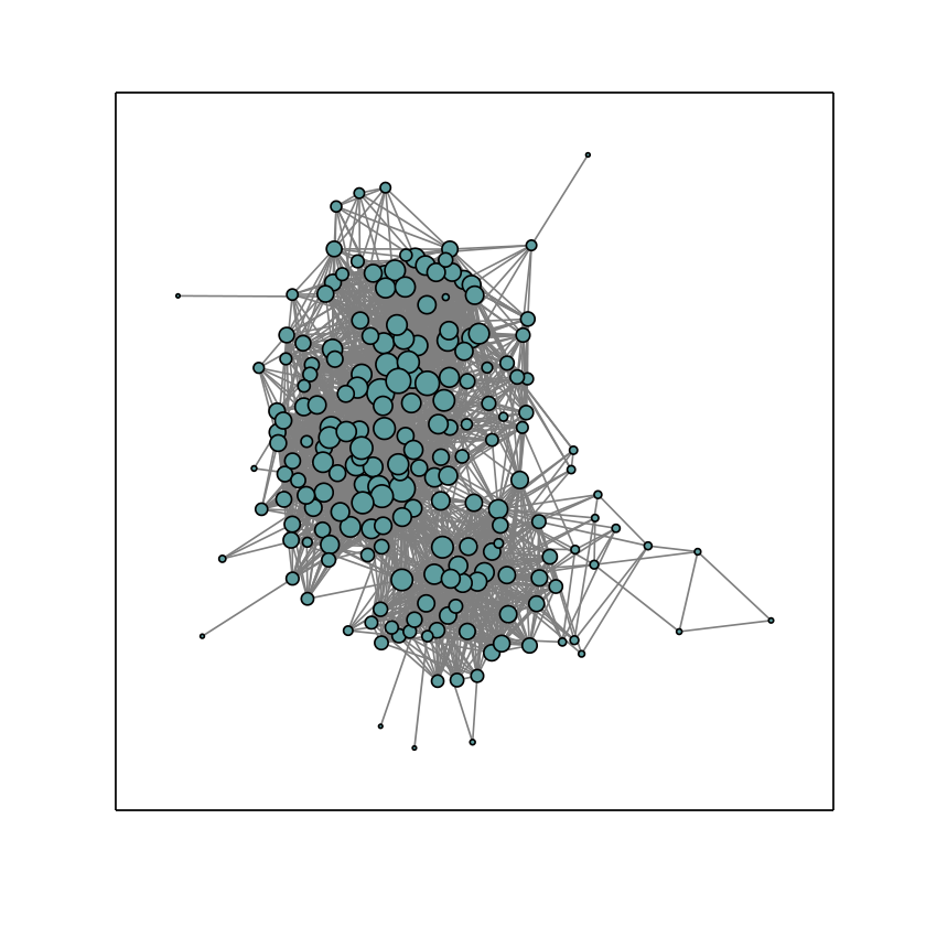
In Figure 2(a-c), node sizes are scaled with their values and the computed centralities give, as expected, the same ranking as effective conductance.
In general, (10) requires modulus computations in all of , while (15) only needs modulus computations in .
Shell modulus centrality can handle fairly large networks, e.g. 100,000 edges. The algorithm used here computes (3) using an active set dual method quadratic programming [15]. It’s theoretically enough to consider at most active constraints [16]. Violated (active) constraints are found using Dijkstra’s algorithm and the constraint matrix is updated using the Cholesky decomposition.
In the following, we focus on approximating (15) efficiently, while incorporating most of the benefits of shell modulus in a scalable framework.
I.1 Bounding from above
First, we provide an upper bound that is known in the complex analysis literature as Ahlfors estimate [17, Chapter 4, Equations 4-6], and in the context of electrical networks goes under the name of Nash-Williams inequality [18]. Given an egonetwork , we consider the set of edges that connect a shell to the next shell , for :
We call the sets shell connecting sets. Since is a minimization problem (3), we get an upper bound simply by choosing an appropriate admissible density . Here, we pick the best admissible density that is constant for all edges in each shell connecting set. After computing the minimized energy of this density, we obtain the following upperbound:
Theorem 2 (Ahlfors upperbound).
Shell modulus is bounded by the following inequality
| (16) |
Proof.
Since (3) is a minimization problem, an upper bound for the shell modulus can be found by picking an appropriate density . Here we will restrict ourselves to densities that are constant on the shell connecting sets . Let
Then we solve the following minimization problem:
| (17) | ||||||
where . By Cauchy-Schwarz inequality
and thus the minimum in 17 is greater than . However, when takes the form:
the minimum is achieved for
∎
I.2 Bounding from below
To provide a lower bound for shell modulus, we focus on geodesic paths (shortest walks). These are usually the most important pathways of influence between the ego and other nodes. Classical measures of centrality, such as closeness centrality and betweenness centrality, are based uniquely on shortest paths [19].
When collecting the egocentric data around an ego , one can take care to avoid forming cycles, and the resulting egonetwork becomes a tree. So assuming is a tree contained in , we can use -monotonicity to get a lower bound, i.e., if , then [5].
Moreover, if we write for the shell modulus of all walks in starting at the root and reaching depth-level , this can be analytically calculated.
Theorem 3.
can be calculated using the following recursive formula.
| (18) |
where are the children of and represents the subtree formed from by keeping only and its descendants.
To prove Equation (18), let be a rooted shortest tree at with vertex set , and edge set . Every density gives a weighted distance on the tree defined by
We define the set of admissible densities Adm, for walks starting from root (ego) to leaves at depth , denoted by
with modulus
Assuming has at least one child, let be the children. Each child induces two rooted subtrees (Figure 3). Let represent the subtree (still rooted at ) formed from by pruning all of ’s children other than along with their descendants, and let represent the subtree (now rooted at ) formed by removing from .
The following lemma is an immediate consequence of the parallel rule of modulus: Given two families and , suppose that and and we have , then .
Lemma 4.
The modulus of is related to the moduli of the as follows.
By Lemma 4, we may restrict ourselves to the case that has a single child . In this case, the serial rule for modulus allows us to reduce the problem to finding the modulus of . This is explained in the following lemma.
Lemma 5.
The modulus of is related to the modulus of as follows.
| (19) |
Proof.
If is a leaf of , then is the minimizer for the modulus. Otherwise, by considering the density, , on the edge from to , the optimization effectively decouples. In order for to be admissible, it is necessary that for every leaf of at depth . For , define the parameterized set of admissible densities, for every leaf
and the parameterized modulus problem
where represents the set of edges in the subtree . It is straightforward to verify that
and, thus
| (20) |
The infimum, given by (19), is attained when
∎
II Shell Degree
In conclusion, Ahlfors’ upper bound (16) considers all edges in the shell connecting sets even if they are not on the shortest paths, such as edge in Figure 4(a). On the other hand, when using the ego-tree approximation, we inevitably lose valuable information hidden in the edges that where discarded. For example, in Figure 4(b-c), to form a tree we need to solve the child custody problem between parents and and child . In particular, the lower bound calculation will discard at least one edge. Moreover, this leads to multiple possible lower bounds, e.g., in Figure 4(b) and for Figure 4(d).
As a compromise between the Ahlfors upper bound and the tree modulus lower bound, we propose a measure we call shell degree. Fix a depth and consider a tree rooted at the ego , whose leaves are all contained in the shell , and such that the geodesics from the root to take exactly hops. Let be the union of all such trees found by breadth first search. For instance, in Figure 4(d) we show in that case. Note that we discarded nodes that are not on the geodesic paths from to .
Since, in general, we cannot use the recursion (18) on , we instead compute the upper bound (16). Namely, we consider the shell connecting sets for and define the generalized shell degree to be the following expression:
| (21) |
Observe that the first summand of (21) is the ordinary degree of the ego and thus our formula acts as a generalization of degree which takes into account information about the shells around the ego. For example, we have , , in Figure 4(d). For , .
We illustrate the differences between (21) with (15), (16), and (18) in Table 1 for the egonetwork in Figure 4.
| Quantity | total | |||
|---|---|---|---|---|
| Lowerbound | ||||
| Upperbpund | ||||
| Shell Degree | ||||
We can compute the summands in (21) with Algorithm 1. Normalization is unnecessary for shell degree, as in the case of degree, which is critical when comparing centrality of different egos and there is no information about connections between their ego-networks.
In short, we keep track of ancestral relations from the ego to nodes in each shells, and discard nodes that do not have any descendants in shell ; leading to required information about and thus we can find summands in (21). The overall time complexity of calculating (21) depends on the graph search in step 4 of Algorithm 1 and keeping the information of ancestral relationships, i.e, for an ego network size , algorithm performance is in .
We illustrate the performance of shell degree compared to the Ahlfors upper bound and the Tree modulus lower bound for conventional random network models such as Erdős-Rényi networks, scale-free (Barabasi-Albert model [20]), Spatial (geometric model in the unit square [21]), and small world (Watts-Strogatz model [22]). Figure 5 shows that shell degree gives a better approximation for than the Ahlfors and Tree modulus estimates.
We see that for egocentric network data with medium sizes and order of neighborhood, shell degree performs extremely well. However, it is possible to produce pathological network examples for which all of the estimates for shell modulus get worse as , see Appendix B for more details.
III Applications of shell degree for targeted immunization strategies
Targeted immunizations in computer networks and human populations can greatly impact the overall outcome of spreading processes [23, 24, 25]. Mitigating an epidemic with random immunization of nodes, requires vaccinating over of the population and thus identifying a good set of target nodes has attracted much attention [26, 27].
Most of the methods for finding good sets of nodes to immunize require global knowledge of the network, making them impossible to use in some practical situations. Therefore, scientists prefer algorithms that are agnostic relative to the global structure of the network. For example, acquaintance immunization chooses random neighbors of randomly picked nodes [28]. In what follows, we illustrate the immunization performance of the approximation of the egocentric version of effective conductance that we call shell degree. We assume , i.e., knowledge of neighbors together with neighbors of neighbors are available. The efficacy of immunization is compared to the popular egocentric measure of acquaintance centrality, and to sociocentric indices such as effective conductance, and betweenness and eigenvector centrality.
We consider the epidemic model “susceptible, infected, recovered” (SIR) that represents infectious processes that are not reversible. Susceptible nodes (S) in the network become infected (I) proportionally to the infectious rate and the number of infected neighbors, and eventually they rest in state (R) after a recovery period of days on average (see Figure 6). We assume a constant , i.e., nodes stay in state (I) an average of 10 days. To model widespread diseases such as the flu that are caused by close contacts, the infectious rate is chosen to have reproduction number , where is the average degree of the network [27].
After updating the contact networks with the immunized nodes, we assess the performance of each strategy. In our experiments, all nodes are initially susceptible and the infectious process starts from a randomly chosen patient zero. The performance of immunization strategies are monitored by measuring the epidemic final size, i.e., number of nodes in state (R) after there is no more (I) nodes.
We simulate the process times for each immunization strategy and each immunization coverage. The simulations are done with GEMFsim, that employs event-based exact stochastic simulation [29] for US power grid and PGP networks, and the friendship network for Princeton University extracted from Facebook [30]. Salathe et. al. [27] suggest considering interactions of individuals in the same dormitory or same year and major, for the Facebook friendship networks, to capture potential physical networks–this makes the networks extremely modular.
In Figure 7, each bar shows the difference of number of cases in the outbreak immunized with the two strategies shown on y-axis for a network. Positive difference (shown in red) means the alternate strategy performs better than shell degree and negative difference (shown in blue) means the shell degree gives better immunization and prevents more cases. We test the significance of comparisons of the obtained results using the nonparametric Mann-Whitney test with [31] and statistically non-significant conclusions are shown by shaded colors.
Effective conductance and betweenness centralitities perform better than shell degree for small immunization coverages. However, using sociocentric centrality measures to design targeted immunization strategies can overlook an important issue, namely, that after removing a fraction of the nodes in the network, the initial ranking by these measures is no longer valid. On the other hand, this is not as dramatic for egocentric measures such as degree, acquaintance, and the egocentric version of effective conductance and the resulting ranking is more robust after changes in the network [10]. Sociocentric measures generally struggle with this fact and thus searching for a good egocentric measure is critical. Therefore, with increasing immunization coverage, shell degree performs better (or similarly) compared to other methods. For strongly modular networks, e.g. the Princeton friendship network, closeness centrality measures are generally less efficient compared to betweenness centrality measures. However, in this case, shell degree is performing better than both eigenvector centrality and acquaintance immunization.
IV Conclusions
In summary, we studied effective conductance centrality in the language of modulus of families of walks and in the context of egocentric networks. We compared our method to its well-known sociocentric counterpart and illustrated the advantages of our approach. For undirected networks, shell modulus can be computed by solving a Laplacian system similar to [33]. Moreover, for directed multi-edge networks, we propose approximations that carry the same benefits of the original definition while being easier to compute and scalable. Finally, we introduced a generalization of degree called shell degree. Applications of these tools illustrate the advantages of the proposed measures, for instance to guide epidemic mitigation strategies under limited knowledge of the overall network.
Acknowledgments
Authors are thankful to NSF grants DMS-1515810 and CIF-1423411.
References
- [1] K. Stephenson and M. Zelen, Social networks 11, 1 (1989).
- [2] D. J. Klein and M. Randić, Journal of mathematical chemistry 12, 81 (1993).
- [3] H. Shakeri, Complex network analysis using modulus of families of walks, Ph.D. thesis, Kansas State University (2017).
- [4] H. Shakeri, P. Poggi-Corradini, N. Albin, and C. Scoglio, Phys. Rev. E 95, 012316 (2017).
- [5] H. Shakeri, P. Poggi-Corradini, C. Scoglio, and N. Albin, Journal of Computational and Applied Mathematics 307, 307 (2016).
- [6] R. J. Duffin, J. Math. Anal. Appl. 5, 200 (1962).
- [7] N. Albin, M. Brunner, R. Perez, P. Poggi-Corradini, and N. Wiens, Conformal Geometry and Dynamics of the American Mathematical Society 19, 298 (2015).
- [8] P. Van Mieghem, K. Devriendt, and H. Cetinay, Physical Review E 96, 032311 (2017).
- [9] J. A. Carrasco, B. Hogan, B. Wellman, and E. J. Miller, Environment and Planning B: Planning and Design 35, 961 (2008).
- [10] E. Costenbader and T. W. Valente, Social networks 25, 283 (2003).
- [11] B. Zemljič and V. Hlebec, Social Networks 27, 73 (2005).
- [12] A. Davis, B. B. Gardner, and M. R. Gardner, Deep South: A social anthropological study of caste and class (Univ of South Carolina Press, 2009).
- [13] D. Lusseau, K. Schneider, O. J. Boisseau, P. Haase, E. Slooten, and S. M. Dawson, Behavioral Ecology and Sociobiology 54, 396 (2003).
- [14] P. M. Gleiser and L. Danon, Advances in complex systems 6, 565 (2003).
- [15] D. Goldfarb and A. Idnani, Mathematical programming 27, 1 (1983).
- [16] N. Albin and P. Poggi-Corradini, The Journal of Analysis 24, 183 (2016).
- [17] L. V. Ahlfors, Conformal invariants: topics in geometric function theory (McGraw-Hill Book Co., New York-Düsseldorf-Johannesburg, 1973) pp. ix+157, mcGraw-Hill Series in Higher Mathematics.
- [18] R. Lyons and Y. Peres, Probability on trees and networks, Vol. 42 (Cambridge University Press, 2016).
- [19] L. C. Freeman, Social networks 1, 215 (1978).
- [20] A.-L. Barabási and R. Albert, Science 286, 509 (1999).
- [21] M. Penrose, Random geometric graphs, 5 (Oxford University Press, 2003).
- [22] D. J. Watts and S. H. Strogatz, nature 393, 440 (1998).
- [23] R. Pastor-Satorras and A. Vespignani, Physical Review E 65, 036104 (2002).
- [24] A. E. Motter and Y.-C. Lai, Physical Review E 66, 065102 (2002).
- [25] M. Zhao, T. Zhou, B.-H. Wang, and W.-X. Wang, Physical Review E 72, 057102 (2005).
- [26] Y. Chen, G. Paul, S. Havlin, F. Liljeros, and H. E. Stanley, Physical review letters 101, 058701 (2008).
- [27] M. Salathé and J. H. Jones, PLoS Comput Biol 6, e1000736 (2010).
- [28] R. Cohen, S. Havlin, and D. Ben-Avraham, Physical review letters 91, 247901 (2003).
- [29] F. D. Sahneh, A. Vajdi, H. Shakeri, F. Fan, and C. Scoglio, arXiv preprint arXiv:1604.02175 (2016).
- [30] A. L. Traud, P. J. Mucha, and M. A. Porter, Physica A: Statistical Mechanics and its Applications 391, 4165 (2012).
- [31] H. B. Mann and D. R. Whitney, The annals of mathematical statistics , 50 (1947).
- [32] M. Boguñá, R. Pastor-Satorras, A. Díaz-Guilera, and A. Arenas, Physical review E 70, 056122 (2004).
- [33] W. Ellens, F. Spieksma, P. Van Mieghem, A. Jamakovic, and R. Kooij, Linear algebra and its applications 435, 2491 (2011).
- [34] D. Spielman, Lecture Notes, Yale University , 740 (2009).
Appendix A Ahlfors upper bound for Erdős-Rényi networks
We want to estimate the expected Ahlfors upper bound in Erdős-Rényi in the connected regime:
We can use the concavity property of Ahlfors bound and get
we would like to estimate .
- •
First, note that is . So:
from the binomial distribution.
- •
Now, given we must toss variables distribute as , because the ego and the first shell are now out of consideration. So
Therefore, computing the second moment of we get:
- •
Given and we must toss a certain number of random variables, where is the number of nodes in the second shell. However, this number is not easy to calculate because it depends on the interaction at the previous step. For instance, if all the binomial variables in the previous step are equal to zero, then . But for higher values of it becomes quite complicated.
In particular, we will have
A.1 Lower bound for
First, we will estimate from below. Given an ego , Spielman [34] sets
and then shows that for ,
He first finds that
| (22) |
and then applies the theory of Chernoff bounds. Note that by simply taking the expectation in (22) we get
This gives geometric growth for :
| (23) |
In our case, since every must toss biased coins, we get
Again, we can take expectations and get
Using (23), we get
A.2 Upper bound for
To get an upper bound we can compare the growth in the Erdős-Rényi graph with the growth for a Galton-Watson branching process with offspring distribution . This will be larger because there are no collisions and we always toss the maximum number of coins. If is the population at time , then
where and we get that
A.2.1 Upper bound for the Ahlfors estimate
We can apply this to our estimate of the average Ahlfors upper bound and get that:
Appendix B Behavior of shell modulus estimates when
B.1 Modulus on the complete graph
Verifying that a metric is extremal for -modulus can be done using Beurling’s criterion (proof in [16]).
Theorem 6 (Beurling’s Criterion for Extremality).
Let be a simple graph, a family of walks on , and . Then, a density is extremal for , if there is a subfamily with for all , such that for all :
| (24) |
The complete graph is a simple graph on nodes, where every node is connected to each other, see Figure 8.

Figure 9 depicts the extremal density for in .

In formulas, for every , and , otherwise is zero. To verify Beurling’s criterion, consider the subfamily of simple paths consisting of and for any . We get that
Take complete graphs .
B.2 Modulus on a chain of complete graphs
Constant sizes
For , assume that , and pick a pair of distinct nodes . Then, for , glue to . We denote the resulting graph by .
For convenience, for , we write , so that the shell at level is . Then, fix , and for , define the following density on :
For , and , set
Observe that the support of can be decomposed as the disjoint union of paths. To see this, enumerate each . Then, for , let
Finally set
One can check that is a Beurling subfamily for the shell modulus . So
which is roughly . Also note that for we recover the degree of . If we sum we get
The Ahlfors upper bound gives
The generalized shell degree, gives
Increasing sizes
Now we repeat the construction above, but this time, setting , we have and, for , we assume that , for an increasing sequence of positive integers .
Then, fix , and for , define the following density on :
For , and , set
Now form paths. Set
As before, enumerate each . Now, , so we can group the edges for into groups of edges. Each such group will then flow through a different node in , and then we repeat. The claim is that this gives rise to a Beurling family of paths . By construction, they all have length equal to . We only need to check Beurling’s criterion. So suppose satisfies
Then is equal to:
And if we write , and collect terms, this equals
which is , because for every
So we get
Now choose . Then
Also
So
And
On the other hand the shell degree is