HoloScope: Topology-and-Spike Aware Fraud Detection
Abstract.
As online fraudsters invest more resources, including purchasing large pools of fake user accounts and dedicated IPs, fraudulent attacks become less obvious and their detection becomes increasingly challenging. Existing approaches such as average degree maximization suffer from the bias of including more nodes than necessary, resulting in lower accuracy and increased need for manual verification. Hence, we propose HoloScope, which uses information from graph topology and temporal spikes to more accurately detect groups of fraudulent users. In terms of graph topology, we introduce “contrast suspiciousness,” a dynamic weighting approach, which allows us to more accurately detect fraudulent blocks, particularly low-density blocks. In terms of temporal spikes, HoloScope takes into account the sudden bursts and drops of fraudsters’ attacking patterns. In addition, we provide theoretical bounds for how much this increases the time cost needed for fraudsters to conduct adversarial attacks. Additionally, from the perspective of ratings, HoloScope incorporates the deviation of rating scores in order to catch fraudsters more accurately. Moreover, HoloScope has a concise framework and sub-quadratic time complexity, making the algorithm reproducible and scalable. Extensive experiments showed that HoloScope achieved significant accuracy improvements on synthetic and real data, compared with state-of-the-art fraud detection methods.
Keywords:
Graph Mining, Fraud Detection, Burst and Drop1. Introduction
Online fraud has become an increasingly serious problem due to the high profit it offers to fraudsters, which can be as much as $5 million from 300 million fake “views” per day, according to a report of Methbot (Ops, 2016) on Dec 2016. Meanwhile, to avoid detection, fraudsters can manipulate their geolocation, internet providers, and IP address, via large IP pools (852,992 dedicated IPs). Suppose a fraudster has accounts or IPs, and wants to rate or click objects (e.g., products) at least 200 times, as required by their customers. The edge density of the fraudulent block is then . We thus see that with enough user accounts or IPs, the fraudsters can serve as many customers as they need while keeping density low. This presents a difficult challenge for most existing fraud detection methods.
Current dense block detection methods (Charikar, 2000; Shin et al., 2016b; Shin et al., 2017) maximize the arithmetic or geometric average degree. We use “fraudulent density” to indicate the edge density that fraudsters create for the target objects. However, those methods have a bias of including more nodes than necessary, especially as the fraudulent density decreases, which we verified empirically. This bias results in low precision, which then requires intensive manual work to verify each user. Fraudar (Hooi et al., 2016) proposed an edge weighting scheme based on inverse logarithm of objects’ degrees to reduce this bias, which was inspired by IDF (Sparck Jones, 1972; Robertson, 2004). However, their weighting scheme is fixed globally and affects both suspicious and normal edges, lowering the precision of Fraudar, which can be seen from results on semi-real (with injected labels) and real data (see Fig. 1).


Accurately detecting fraudulent blocks of lower density requires aggregating more sources of information. Consider the attribute of the creation time of edges: fraudulent attacks tend to be concentrated in time, e.g., fraudsters may surge to retweet a message, creating one or more sudden bursts of activity, followed by sudden drops after the attack is complete. Sudden bursts and drops have not been directly considered together in previous work.
Tensor based methods (Jiang et al., 2015; Shin et al., 2016b; Shin et al., 2017) incorporate edge attributes into a multi-way tensor formulation, e.g., IPs, rating scores and time. However, those methods rely on time-binning to incorporate temporal information, and then treat time bins independently, which loses information about bursts and drops, which our approach captures.
Therefore, we propose HoloScope, which combines suspicious signals from graph topology, temporal bursts and drops, and rating deviation. Our graph topology-based weighting scheme dynamically reweights objects according to our beliefs about which users are suspicious. Temporally, HoloScope detects suspicious spikes of bursts and drops, which increases the time cost needed for fraudsters to conduct an attack. In terms of rating deviation, our approach takes into account how much difference there is between an object’s ratings given by suspicious users and non-suspicious users.
In summary, our contributions are:
- •
Unification of signals: we make holistic use of several signals, namely connectivity (i.e., topology), temporal bursts and drops, and rating deviation in a systematic way.
- •
Theoretical analysis of fraudsters’ obstruction: we show that if the fraudsters use less than an upper bound of time for an attack, they will cause a suspicious drop or burst. In other words, HoloScope obstructs fraudsters by increasing the time they need to perform an attack.
- •
Effectiveness: we achieved higher accuracy than the competitors on semi-real and real datasets. In fact, HoloScope using only topology information (HS-) outperformed the graph-based competitors (see Fig. 1(a)), while HoloScope (HS) using all attributes achieved further improvement, and outperformed the tensor-based competitors (see Fig. 1(b) and 1(c)).
- •
Scalability: HoloScope runs in subquadratic time in the number of nodes, under reasonable assumptions. Fig. 2 shows that its running time increases near-linearly with the number of edges.
In addition, in Microblog, Sina Weibo11 1 The largest Microblog service in China, http://www.weibo.com data, HoloScope achieved higher F-measure than the competitors in detecting the ground truth labels, with high precision and recall. The code of HoloScope is open-sourced for reproducibility 22 2 https://github.com/shenghua-liu/HoloScope.
|
Fraudar (Hooi et al., 2016) |
SpokEn (Prakash et al., 2010) |
CopyCatch (Beutel et al., 2013) |
CrossSpot (Jiang et al., 2015) |
BP-based methods (Pandit et al., 2007; Akoglu et al., 2013) |
M-Zoom/D-Cube (Shin et al., 2016b; Shin et al., 2017) |
HoloScope | |
| scalability | ✓ | ✓ | ✓ | ✓ | ✓ | ✓ | ✓ |
| camouflage | ✓ | ? | ✓ | ✓ | ✓ | ||
| hy-community | ? | ? | ✓ | ||||
| spike-aware | ? | ✓ |
2. Related Works
Most existing works study anomaly detection based on the density of blocks within adjacency matrices (Prakash et al., 2010; Jiang et al., 2014), or multi-way tensors (Shin et al., 2016b; Shin et al., 2017). (Gibson et al., 2005) and CoreScope (Shin et al., 2016a) proposed to use Shingling and K-core algorithms respectively to detect anomalous dense block in huge graphs. Taking into account the suspiciousness of each edge or node in a real life graph potentially allows for more accurate detection. Fraudar (Hooi et al., 2016) proposed to weight edges’ suspiciousness by the inverse logarithm of objects’ indegrees, to discount popular objects. (Araujo et al., 2014) found that the degrees in a large community follow a power law distribution, forming hyperbolic structures. This suggests penalizing high degree objects to avoid unnecessarily detecting the dense core of hyperbolic community.
In addition to topological density, EdgeCentric (Shah et al., 2015) studied the distribution of rating scores to find the anomaly. In terms of temporal attribute, the identification of burst period has been studied in (Kumar et al., 2005). A recent work, Sleep Beauty (SB) (Ke et al., 2015) more intuitively defined the awakening time for a paper’s citation burst for burst period. (Yang and Leskovec, 2011) clustered the temporal patterns of text phrases and hash tags in Twitter. Meanwhile, (Günnemann et al., 2014b; Günnemann et al., 2014a) modeled the time stamped rating scores with Bayesian model and autoregression model respectively for anomalous behavior detection. Even though (Xie et al., 2012; Li et al., 2016; Fei et al., 2013) have used bursty patterns to detect review spam, a sudden drop in temporal spikes has not been considered yet.
However, aggregating suspiciousness signals from different attributes is challenging. (Cormack et al., 2009) proposed RRF (Reciprocal Rank Fusion) scores for combining different rank lists in information retrieval. However, RRF applies to ranks, not suspiciousness scores.
CrossSpot (Jiang et al., 2015), a tensor-based algorithm, estimated the suspiciousness of a block using a Poisson model. However, it did not take into account the difference between popular and unpopular objects. Moreover, although CrossSpot, M-Zoom (Shin et al., 2016b) and D-Cube (Shin et al., 2017) can consider edge attributes like rating time and scores via a multi-way tensor approach, they require a time-binning approach. When time is split into bins, attacks which create bursts and drops may not stand out clearly after time-binning. The problem of choosing bin widths for histograms was studied by Sturges (Sturges, 1926) assuming an approximately normal distribution, and Freedman-Diaconis (Freedman and Diaconis, 1981) based on statistical dispersion. However, the binning approaches were proposed for the time series of a single object, which is not clear for different kinds of objects in a real life graph, namely, popular products and unpopular products should use different bin sizes.
Belief propagation (Pandit et al., 2007) is another common approach for fraud detection which can incorporate some specific edge attributes, like sentiment (Akoglu et al., 2013). However, its robustness against adversaries which try to hide themselves is not well understood.
CopyCatch (Beutel et al., 2013) detected lockstep behavior by maximizing the number of edges in blocks constrained within time windows. However, this approach ignores the distribution of edge creation times within the window, and does not capture bursts and drops directly.
Finally, we summarize our competitors compared to our HoloScope in Table 1. We use “hy-community” to indicate whether the method can avoid detecting the naturally-formed hyperbolic topology which is unnecessary for fraud detection. HoloScope is the only one which considers temporal spikes (sudden bursts and drops and multiple bursts) and hyperbolic topology, in a unified suspiciousness framework.
3. Proposed Approach
The definition of our problem is as follows.
Problem 1 (informal definition).
Given quadruplets (, , , , where is the time that a rates an , and is the categorical rating scores.
- -
Find a group of suspicious users, and suspicious objects or its rank list with suspiciousness scores,
- -
to optimize the metric under the common knowledge of suspiciousness from topology, rating time and scores.
To make the problem more general, and are optional. For example, in Twitter, we have triples, where retweets a message at . In a static following network, we have pairs , with following .
As discussed in previous sections, our metric should capture the following basic traits:
Trait 1 (Engagement).
Fraudsters engage as much firepower as possible to boost customers’ objects, i.e., suspicious objects.
Trait 2 (Less Involvement).
Suspicious objects seldom attract non-fraudulent users to connect with them.
Trait 3 (Spikes: Bursts and Drops).
Fraudulent attacks are concentrated in time, sometimes over multiple waves of attacks, creating bursts of activity. Conversely, the end of an attack corresponds to sudden drops in activity.
Trait 4 (Rating Deviation).
High-rating objects seldom attract extremely low ratings from normal users. Conversely, low-rating objects seldom attract extremely high ratings from normal users.
Thus we will show in the following sections, that our proposed metric can make holistic use of several signals, namely topology, temporal spikes, and rating deviation, to locate suspicious users and objects satisfying the above traits. That is the reason we name our method as HoloScope (HS).
3.1. HoloScope metric
To give a formal definition of our metric, we describe the quadruplets (, , , ) as a bipartite and directed graph , which is the source node set, is the sink node set, and connections is the directed edges from to . Generally, graph is a multigraph, i.e., multiple edges can be present between two nodes. Multiple edges mean that a user can repeatedly comment or rate on the same product at a different time, as common in practice. Users can also retweet message multiple times in the Microblog . Each edge can be associated with rating scores (), and timestamps, for which the data structure is introduced in Subsection 3.1.2.
Our HoloScope metric detects fraud from three perspectives: topology connection, timestamps, and rating score. To easily understand the framework, we first introduce the HoloScope in a perspective of topology connection. Afterwards, we show how we aggregate the other two perspectives into the HoloScope. We first view as a weighted adjacency matrix , with the number of multiple edges (i.e., edge frequency) as matrix elements.
Our goal is to find lockstep behavior of a group of suspicious source nodes who act on a group of sink nodes . Based on Trait 1, the total engagement of source nodes to sink nodes can be basically measured via density measures. There are many density measures, such as arithmetic and geometric average degree. Our HoloScope metric allows for any such measure. However, as the average degree metrics have a bias toward including too many nodes, we use a measure denoted by as the basis of the HoloScope, defined as:
| (1) |
where is the total edge frequency from source nodes to a sink node . can also be viewed as an engagement from to , or ’s lockstep on , which is defined as
| (2) |
where constant are the global suspiciousness on an edge, and is the element of adjacency matrix , i.e., the edge frequency between a node pair . The edge frequency becomes a binary in a simple graph. The global suspiciousness as a prior can come from the degree, and the extra knowledge on fraudsters, such as duplicated review sentences and unusual behaving time.
To maximize , the suspicious source nodes and the suspicious sink nodes are mutually dependent. Therefore, we introduce contrast suspiciousness in an informal definition:
Definition 3.1 (contrast suspiciousness).
The contrast suspiciousness denoted as is defined as the conditional likelihood of a sink node that belongs to (the suspicious object set), given the suspicious source nodes .
A visualization of the contrast suspiciousness is given in Fig. 3. The intuitive idea behind contrast suspiciousness is that in the most case, we need to judge the suspiciousness of objects by currently chosen suspicious users , e.g., an object is more suspicious if very few users not in are connected to it (see Trait 2); the sudden burst of an object is mainly caused by (see Trait 3); or the rating scores from to an object are quite different from other users (see Trait 4). Therefore, such suspiciousness makes use of the contrasts between users in and users not in or the whole set.

Finally, instead of maximizing , we maximize the following expectation of suspiciousness over the probabilities :
| (3) |
where for simplicity we write to mean . is the probability of being a normal sink node. We dynamically calculate the contrast suspiciousness for all the objects, after every choice of source nodes .
Using this overall framework for our proposed metric , we next show how to satisfy the remaining Traits. To do this, we define contrast suspiciousness in a way that takes into account various edge attributes. This will allow greater accuracy particularly for detecting low-density blocks.
3.1.1. HS-: Less involvement from others.
Based on Trait 2, a sink node should be more suspicious if it only attracts connections from the suspicious source nodes , and less from other nodes. Mathematically, we capture this by defining
| (4) |
where is the weighted indegree of sink node . Similar to , the edges are weighted by global suspiciousness. measures the involvement ratio of in the activity of sink node . The scaling function is our belief about how this ratio relates to suspiciousness, and we choose the exponential form , where base .
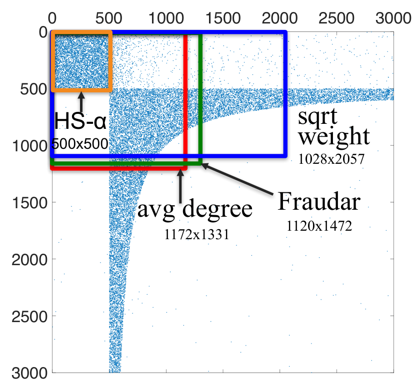

As previous work showed, large communities form hyperbolic structures, which is generated in our synthetic data (see the lower-right block in Fig. 4(a)), and also exists in real BeerAdvocate data (see Fig. 4(b)). For clarity, our HoloScope method are denoted as HS- when it is only applied on a connection graph. The results of the synthetic data show that HS- detected the exact dense rectangular block (), while the other competitors included a lot of non-suspicious nodes from the core part of hyperbolic community resulting in low accuracy. In the beer review data from the BeerAdvocate website, testing on different fraudulent density (see Fig. 1(a)), our HS- remained at high accuracy, while the other methods’ accuracy drops quickly when the density drops below 70%.
The main idea is that HS- can do better because it dynamically adjusts the weights for sink nodes, penalizing those sink nodes that also have many connections from other source nodes not in . In contrast, although Fraudar proposed to penalize popular sink nodes based their indegrees, these penalties also scaled down the weights of suspicious edges. The Fraudar (green box) only improved the unweighted “average degree” method (red box) by a very limited amount. Moreover, with a heavier penalty, the “sqrt weight” method (blue box) achieved better accuracy on source nodes but worse accuracy on sink nodes, since those methods used globally fixed weights, and the weights of suspicious were penalized as well. Hence the hyperbolic structure pushes those methods to include more nodes from its core part.
In summary, our HS- using dynamic contrast suspiciousness can improve the accuracy of fraud detection in ‘noisy’ graphs (containing hyperbolic communities), even with low fraudulent density.


3.1.2. Temporal bursts and drops
Timestamps for edge creation are commonly available in most real settings. If two subgroups of Microblog users have the same number of retweets to a message, can we say they have the same suspiciousness? As an example shown in Fig. 5(a), the red line is the time series (histogram of time bins) of the total retweets of a message in Microblog, Sina Weibo. The blue dotted line and green dashed line are the retweeting time series respectively from user groups and . The two series have the same area under the time series curves, i.e., the same number of retweets. However, considering that fraudsters tend to surge to retweet a message to reduce the time cost, the surge should create one or more sudden bursts, along with sudden drops. Therefore, the suspiciousness of user groups and become quite different even though they have the same number of retweets, which cannot be detected solely based on connections in the graph. Thus we include the temporal attribute into our HoloScope framework for defining contrast suspiciousness.
Denote the list of timestamps of edges connected to a sink node as . To simplify notation, we use without subscript when talking about a single given sink node . Let ={(, ), (, ), , (, )} as the time series of , i.e., the histogram of . The count is the number of timestamps in the time bin , with bin size . The bin size of histogram is calculated according to the maximum of Sturges criteria and the robust Freedman-Diaconis’ criteria as mentioned in related works. It is worth noticing that the HoloScope can tune different bin sizes for different sink nodes, e.g., popular objects need fine-grained bins to explore detailed patterns. Hence, the HoloScope is more flexible than tensor based methods, which use a globally fixed bin size. Moreover, the HoloScope can update the time series at a low cost when is increasing.
To consider the burst and drop patterns described in Trait 3, we need to decide the start point of a burst and the end point of a drop in time series . Let the burst point be (, ), having the maximum value . According to the definition in previous work “Sleeping Beauty”, we use an auxiliary straight line from the beginning to the burst point to decide the start point, named the awakening point of the burst. Fig. 5(b) shows the time series (red polygonal line) of a message from Sina Weibo, the auxiliary straight line (black dotted line) from the lower left point (, ) to upper right point (, ), and the awakening point for the maximum point (, ), which is defined as the point along the time series which maximizes the distance to . As the dotted line perpendicular to suggests in this figure, the awakening point satisfies
| (5) |
Finding the awakening point for one burst is not enough, as multiple bursts may be present. Thus, sub-burst points and the associated awakening points should be considered. We then propose a recursive algorithm in Alg. 1 for such a purpose.
After finding awakening and burst points, the contrast suspiciousness of burst awareness satisfies , where is the involvement ratio of source nodes in in multiple bursts. Let the collection of timestamps from to sink node be . Then,
| (6) |
where is the slope from the output of algorithm. Here is used as a weight based on how steep the current burst is. This definition of suspiciousness satisfies Trait 3. It is worth noticing that the algorithm only needs to be executed once. With the preprocessed awakening and burst points, the contrast suspiciousness of edges connected to has complexity, where is the degree of sink node . Hence the complexity for overall sink nodes are .
In fact, sudden drops are also a prominent pattern of fraudulent behavior as described in Trait 3, since after creating the attack is complete, fraudsters usually stop their activity sharply. To make use of the suspicious pattern of a sudden drop, we define the as the end of a drop. As Fig. 5(b) suggests, another auxiliary straight line is drawn from the highest point (, ) to the last point (, ). The dying point (, ) can be found by maximizing the distance to this straight line. Thus we can discover the “sudden drop” by the absolute slope value = between the burst point and the dying point. Since there may be several drops in a fluctuated time series , we choose the drop with the maximum fall. To find the maximum fall, we also need a recursive algorithm, similar to Alg. 1:
1) Find a maximum point (, ), and the corresponding dying point (, ) by definition; 2) Calculate the current drop slope , and the drop fall = ; 3) Recursively find drop slope and drop fall for the left and right parts of , i.e., and respectively.
As a result, the algorithm returns the maximum drop fall , and its drop slope , which it has found recursively. Finally, we use the weighted drop slope as a global suspiciousness in equation (2), to measure the drop suspiciousness. Each edge connected to the sink node is assigned the same drop suspiciousness. We use a logarithm scale for smoothing those edge weights.
With this approach to detect bursts and drops, we now show that this provides a provable time obstruction for fraudsters.
Theorem 3.2.
Let be the number of edges that fraudsters want to create for an object. If the fraudsters use time less than , then they will be tracked by a suspicious burst or drop, where is the size of time bins, and and are the slopes of normal rise and decline respectively.
Proof.
The most efficient way to create edges is to have one burst and one drop, otherwise more time is needed. As shown in Fig. 5(c), in order to minimize the slope, every point in the time series should in line with the two auxiliary straight lines to the highest point , separately from the awakening and dying points. Otherwise, the slopes will exceed the normal values and . Hence we only consider the triangle with the auxiliary lines as its two edges. It is worth noticing that a trapezoid whose legs have the same slopes as the triangle’s edges cannot have a shorter time cost. Then
Here and are the number of time bins before and after the burst. is the total number of rating edges, and consider some edges from normal users. Thus, solving the above equations, we have
∎
3.1.3. Rating deviation and aggregation
We now consider edges with categorical attributes such as rating scores, text contents, etc. For each sink node , we use the KL-divergence between the distributions separately from the suspicious source nodes and the other nodes, i.e., . We use for KL-divergence instead of the whole source nodes , in order to avoid the trivial case where most of the rating scores are from . The rating deviation is scaled into by the maximum value before being passed into function to compute contrast suspiciousness. The neutral scores can be ignored in the KL-divergence for the purpose of detecting fraudulent boosting or defamation. Moreover, rating deviation is meaningful when both and have the comparable numbers of ratings. Thus, we weighted by a balance factor, , .
To make holistic use of different signals, i.e., topology, temporal spikes, and rating deviation, we need a way to aggregate those signals together. We have tried to use RRF (Reciprocal Rank Fusion) scores from Information Retrieval, and wrapped the scores with and without scaling function . Compared to RRF score, we found that a natural way of joint probability by multiplying those signals together:
| (7) |
was the most effective way to aggregate. In a joint probability, we can consider the absolute suspicious value of each signal, as opposite to the only use of ranking order. Moreover, being wrapped with , the signal values cannot be canceled out by multiplying a very small value from other signals. A concrete example is that a suspicious spike can still keep a high suspiciousness score by multiplying a very small score from low fraudulent density.
Moreover, HoloScope dynamically updates the contrast suspiciousness . Thus the sink nodes being added with camouflage will have a very low contrast suspiciousness, with respect to the suspicious source nodes . This offers HoloScope the resistance to camouflage.
3.2. Algorithm
Before designing the full algorithm for large scale datasets, we firstly introduce the most important sub-procedure in Alg. 2.
At the beginning, this greedy shaving procedure starts with an initial set as input. It then greedily deletes source nodes from , according to users’ scores :
which can be interpreted as how many suspicious nodes that user is involved in. So the user is less suspicious if he has a smaller score, with respect to the current contrast suspiciousness , where we use to denote a vector of contrast suspiciousness of all sink nodes. We build a priority tree to help us efficiently find the user with minimum score. The priority tree updates the users’ scores and maintains the new minimum as the priorities change. With removing source nodes , the contrast suspiciousness change, in which we then update users’ scores . The algorithm keeps reducing until it is empty. The best maximizing objective and are returned at the end.
Since awakening and burst points have been already calculated for each sink node as an initial step before the procedure, the calculation of the contrast suspicious for a sink node only needs time. With source node as the -th one removed from by the procedure, , and the out degree as , the complexity is
| (8) |
where is the set of edges connected to source nodes .
With the procedure, our scalable algorithm can be designed so as to generate candidate suspicious source node sets. In our implementation, we use singular vector decomposition (SVD) for our algorithm. Each top singular vector gives a spectral view of high connectivity communities. However, those singular vectors are not associated with suspiciousness scores. Thus combined with the top singular vectors, our fast greedy algorithm is given in Alg. 3.
Theorem 3.3 (Algorithm complexity).
In the graph , given and , the complexity of algorithm is subquadratic, i.e., in little-o notation, if the size of truncated user set , where .
Proof.
The algorithm executes in a constant iterations. is assigned to in every procedure. Then . In the adjacency matrix of the graph, we consider the submatrix with as rows and as columns. If the fraudulent dense block is in submatrix , then we assume that the block has at most columns. Excluding the dense block, the remaining part of is assumed to have the same density with the whole matrix . Therefore, the total number of edges in is
Then based on equation (8), the algorithm complexity is
Therefore, if , then the complexity is subquadratic . ∎
In real life graph, , so if the complexity of algorithm is subquadratic. Therefore, without loss of performance and efficiency, we can limit for truncating an ordered in the algorithm for a large dataset.
In algorithm for HS-, SVD on adjacency matrix is used to generate initial blocks for the procedure. Although we can still use SVD on for HS with holistic attributes, yet considering attributes of timestamps and rating scores may bring more benefits. Observing that not every combination of # of stars, timestamps and product ids has a value in a multi-way tenor representation, we can only choose every existing triplets (, , ) as one column, and as rows, to form a new matrix. The above transformation is called the of a tensor, which outputs a new matrix. With proper time bins, e.g., one hour or day, and re-clustering of , the flattening matrix becomes more dense and contains more attribute information. Thus we use such a flattening matrix with each column weighted by the sudden-drop suspiciousness for our algorithm.
4. Experiments
| Data Name | #nodes | #edges | time span |
| BeerAdvocate (McAuley and Leskovec, 2013b) | 26.5K x 50.8K | 1.07M | Jan 08 - Nov 11 |
| Yelp | 686K x 85.3K | 2.68M | Oct 04 - Jul 16 |
| Amazon Phone & Acc (McAuley and Leskovec, 2013a) | 2.26M x 329K | 3.45M | Jan 07 - Jul 14 |
| Amazon Electronics (McAuley and Leskovec, 2013a) | 4.20M x 476K | 7.82M | Dec 98 - Jul 14 |
| Amazon Grocery (McAuley and Leskovec, 2013a) | 763K x 165K | 1.29M | Jan 07 - Jul 14 |
| Amazon mix category (Mukherjee et al., 2012) | 1.08M x 726K | 2.72M | Jan 04 - Jun 06 |
| Data Name | metrics* | source nodes | sink nodes | ||||||
| M-Zoom | D-Cube | CrossSpot | HS | M-Zoom | D-Cube | CrossSpot | HS | ||
| BeerAdvocate | auc | 0.7280 | 0.7353 | 0.2259 | 0.9758 | 0.6221 | 0.6454 | 0.1295 | 0.9945 |
| F90% | 0.5000 | 0.5000 | – | 0.0333 | 0.5000 | 0.5000 | – | 0.0333 | |
| Yelp | auc | 0.9019 | 0.9137 | 0.9916 | 0.9925 | 0.9709 | 0.8863 | 0.0415 | 0.9950 |
| F90% | 0.2500 | 0.2000 | 0.0200 | 0.0143 | 0.0250 | 1.0000 | – | 0.0100 | |
| Amazon | auc | 0.9246 | 0.8042 | 0.0169 | 0.9691 | 0.9279 | 0.8810 | 0.0515 | 0.9823 |
| Phone & Acc | F90% | 0.1667 | 0.5000 | – | 0.0200† | 0.1429 | 0.1000 | – | 0.0200† |
| Amazon | auc | 0.9141 | 0.9117 | 0.0009 | 0.9250 | 0.9142 | 0.7868 | 0.0301 | 0.9385 |
| Electronics | F90% | 0.2000 | 0.1250 | – | 0.1000 | 0.1000 | 0.5000 | – | 0.1250 |
| Amazon | auc | 0.8998 | 0.8428 | 0.0058 | 0.9250 | 0.8756 | 0.8241 | 0.0200 | 0.9621 |
| Grocery | F90% | 0.1667 | 0.5000 | – | 0.1000 | 0.1250 | 0.2500 | – | 0.1000 |
| Amazon | auc | 0.9001 | 0.8490 | 0.5747 | 0.9922 | 0.9937 | 0.9346 | 0.0157 | 0.9950 |
| mix category | F90% | 0.2500 | 0.5000 | 0.2000† | 0.0167 | 0.0100 | 0.2000 | – | 0.0100 |
- •
* we use the two metrics: the area under the curve (abbrev as low-case “auc”) of the accuracy curve as drawn in Fig. 1(b), and the lowest density that the method can detect in high accuracy().
- •
† one of the above fraudulent density was not detected in high accuracy.
In the experiments, we only consider the significant multiple bursts for fluctuated time series of sink nodes. We keep those awakening-burst point pairs with the altitude difference at least 50% of the largest altitude difference in the time series. Table 2 gives the statistics of our six datasets which are publicly available for academic research 33 3 Yelp dataset is from https://www.yelp.com/dataset_challenge . Our extensive experiments showed that the performance was insensitive to scaling base , and became very stable when larger than 32. Hence we choose in the following experiments.
4.1. Evaluation on different injection density
In the experiments, we mimic the fraudsters’ behaviors and randomly choose 200 objects that has no more than 100 indegree as the fraudsters’ customers, since less popular objects are more likely to buy fake ratings. On the other hand, the fraudulent accounts can come from the hijacked user accounts. Thus we can uniformly sample out a number of users from the whole user set as fraudsters. To test on different fraudulent density, the number of sampled fraudsters ranges from 200 to 20000. Those fraudsters as a whole randomly rate each of the 200 products for 200 times, and also create some biased camouflage on other products. As a results, the fraudulent density ranges from 1.0 to 0.01 for testing. The rating time was generated for each fraudulent edge: first randomly choosing a start time between the earliest and the latest creation time of the existing edges; and then plus a randomly and biased time interval from the intervals of exiting creation time, to mimic the surge of fraudsters’ attacks. Besides, a high rating score, e.g. 4 or 4.5, is randomly chosen for each fraudulent edge44 4 the injection code is also open-sourced for reproducibility.
Fig. 1(b) shows the results of HoloScope HS on the BeerAdvocate data. When the fraudulent density decreases from the right to the left along the horizontal axis, HS can keep as high F-measure on accuracy as more than 80% before reaching 0.025 in density, better by far than the competitors. Since HS returns suspiciousness scores for sink nodes, we measure their accuracy using AUC (the area under the ROC curve), where ROC stands for receiver operating characteristic. For the detection of suspicious objects, HS achieved more than 0.95 in AUC for all the testing injection density, with a majority of tests reaching to 1.0.
In order to give a comparison on all six data sets with different injection density, we propose to use the two metrics: a low-case “auc” and the lowest density, described in the notes of Table 3. The table reports the fraud detection results of our HoloScope (HS) and competitors on the six datasets. Since the accuracy curve stops at 0.01 (the minimum testing density); and we add zero accuracy at zero density, the ideal value of auc is 0.995. The auc on source and sink nodes are reported separately. As the table suggests, our HS achieved the best auc among the competitors, and even reached the ideal auc in two cases. Since the HS outputs the suspiciousness scores for sink nodes, we used the area under the upper-case AUC (similar to F-measure) accuracy curve along all testing density. Although it is sometimes unfair to compare F-measure with AUC, since the smallest value of AUC is around 0.5, yet the high auc values can indicate the high F-measure values on our top suspicious list.
Furthermore, we compare the lowest density in Table 3. The better a method is, the lower density it should be able to detect well. As we can see, HS has the smallest detection density in most cases, which can be as small as 0.0143 on source nodes, and reached the minimum testing density of 0.01 on sink nodes. That means we can detect fraudsters in high accuracy even if they use 14 thousand accounts to create 200 200 fake edges for 200 objects. The fraudulent objects can also be detected accurately, even if 20 thousand fraudsters are hired to create 200 fake edges for each object.
4.2. Evaluation on Sina Weibo with real labels
We also did experiments on a large real dataset from Sina Weibo, which has 2.75 million users, 8.08 million messages, and 50.1 million edges in Dec 2013. The user names and ids, and message ids are from the online system. Thus we can check their existence status in the system to evaluate the experiments. If the messages or the users were deleted from the system, we treat them as the basis for identifying suspicious users and messages. Since it is impossible to check all of the users and messages, we firstly collected a candidate set, which is the union of the output sets from the HS and the baseline methods. The real labels are from the candidate set by checking the status whether they still exists in Sina Weibo (checked in Feb. 2017). We used a program on the API service of Sina Weibo to check the candidate user and message id lists, finally resulting in 3957 labeled users and 1615 labeled messages.
The experimental results in Fig. 1(c) show that HS achieved high F-measure on accuracy, which detected 3781 labeled users higher than M-Zoom’s 1963 labeled users. The F-measure of HS improved about 30% and 60%, compared with M-Zoom and D-Cube respectively. CrossSpot biased to include a large amount of users in their detection results, which detected more than 100 labeled users but with extremely low precision, i.e., less than 1%. That is the reason CrossSpot got the lowest F-measure, which is less than 1.5%. For labeled messages, the HS achieved around 0.8 in AUC, while M-Zoom and D-Cube got lower recall, and CrossSpot still suffered very low F-measure with higher recall. Therefore, our HoloScope outperformed the competitors in real-labeled data as well.
4.3. Scalability
To verify the complexity, we choose two representative datasets: BeerAdvocate data which has the highest volume density, and Amazon Electronics which has the most edges. We truncated the two datasets according to different time ranges, i.e., from the past 3 months, 6 months, or several years to the last day, so that the generated data size increases. Our algorithm is implemented in Python. As shown in Fig. 2, the running time of our algorithm increases almost linearly with the number of the edges.
5. Conclusion
We proposed a fraud detection method, HoloScope, on a bipartite graph which can have timestamps and rating scores. HoloScope has the following advantages: 1) Unification of signals: we make holistic use of several signals, namely topology, temporal spikes, and rating deviation in our suspiciousness framework in a systematic way. 2) Theoretical analysis of fraudsters’ obstruction: we showed that if the fraudsters use less than an upper bound of time to rate an object, they will cause a suspicious drop or burst. In other words, our HoloScope can obstruct fraudsters and increases their time cost. 3) Effectiveness: we achieved higher accuracy on both semi-real and real datasets than the competitors, achieving good accuracy even when the fraudulent density is low. 4) Scalability: while HoloScope needs to dynamically update the suspiciousness of objects, the algorithm is sub-quadratic in the number of nodes, under reasonable assumptions.
References
- Akoglu et al. (2013) Leman Akoglu, Rishi Chandy, and Christos Faloutsos. 2013. Opinion Fraud Detection in Online Reviews by Network Effects. ICWSM 13 (2013), 2–11.
- Araujo et al. (2014) Miguel Araujo, Stephan Günnemann, Gonzalo Mateos, and Christos Faloutsos. 2014. Beyond blocks: Hyperbolic community detection. In Joint European Conference on Machine Learning and Knowledge Discovery in Databases. Springer, 50–65.
- Beutel et al. (2013) Alex Beutel, Wanhong Xu, Venkatesan Guruswami, Christopher Palow, and Christos Faloutsos. 2013. Copycatch: stopping group attacks by spotting lockstep behavior in social networks. In Proceedings of the 22nd international conference on World Wide Web. ACM, 119–130.
- Charikar (2000) Moses Charikar. 2000. Greedy approximation algorithms for finding dense components in a graph. In International Workshop on Approximation Algorithms for Combinatorial Optimization. Springer, 84–95.
- Cormack et al. (2009) Gordon V Cormack, Charles LA Clarke, and Stefan Buettcher. 2009. Reciprocal rank fusion outperforms condorcet and individual rank learning methods. In Proceedings of the 32nd international ACM SIGIR conference on Research and development in information retrieval. ACM, 758–759.
- Fei et al. (2013) Geli Fei, Arjun Mukherjee, Bing Liu, Meichun Hsu, Malu Castellanos, and Riddhiman Ghosh. 2013. Exploiting Burstiness in Reviews for Review Spammer Detection. ICWSM 13 (2013), 175–184.
- Freedman and Diaconis (1981) David Freedman and Persi Diaconis. 1981. On the histogram as a density estimator: L 2 theory. Probability theory and related fields 57, 4 (1981), 453–476.
- Gibson et al. (2005) David Gibson, Ravi Kumar, and Andrew Tomkins. 2005. Discovering large dense subgraphs in massive graphs. In Proceedings of the 31st international conference on Very large data bases. VLDB Endowment, 721–732.
- Günnemann et al. (2014a) Nikou Günnemann, Stephan Günnemann, and Christos Faloutsos. 2014a. Robust multivariate autoregression for anomaly detection in dynamic product ratings. In Proceedings of the 23rd international conference on World wide web. ACM, 361–372.
- Günnemann et al. (2014b) Stephan Günnemann, Nikou Günnemann, and Christos Faloutsos. 2014b. Detecting anomalies in dynamic rating data: A robust probabilistic model for rating evolution. In Proceedings of the 20th ACM SIGKDD international conference on Knowledge discovery and data mining. ACM, 841–850.
- Hooi et al. (2016) Bryan Hooi, Hyun Ah Song, Alex Beutel, Neil Shah, Kijung Shin, and Christos Faloutsos. 2016. Fraudar: bounding graph fraud in the face of camouflage. In Proceedings of the 22nd ACM SIGKDD International Conference on Knowledge Discovery and Data Mining. ACM, 895–904.
- Jiang et al. (2015) Meng Jiang, Alex Beutel, Peng Cui, Bryan Hooi, Shiqiang Yang, and Christos Faloutsos. 2015. A general suspiciousness metric for dense blocks in multimodal data. In Data Mining (ICDM), 2015 IEEE International Conference on. IEEE, 781–786.
- Jiang et al. (2014) Meng Jiang, Peng Cui, Alex Beutel, Christos Faloutsos, and Shiqiang Yang. 2014. Inferring strange behavior from connectivity pattern in social networks. In Pacific-Asia Conference on Knowledge Discovery and Data Mining. Springer, 126–138.
- Ke et al. (2015) Qing Ke, Emilio Ferrara, Filippo Radicchi, and Alessandro Flammini. 2015. Defining and identifying Sleeping Beauties in science. Proceedings of the National Academy of Sciences 112, 24 (2015), 7426–7431.
- Kumar et al. (2005) Ravi Kumar, Jasmine Novak, Prabhakar Raghavan, and Andrew Tomkins. 2005. On the bursty evolution of blogspace. World Wide Web 8, 2 (2005), 159–178.
- Li et al. (2016) Huayi Li, Geli Fei, Shuai Wang, Bing Liu, Weixiang Shao, Arjun Mukherjee, and Jidong Shao. 2016. Modeling Review Spam Using Temporal Patterns and Co-bursting Behaviors. arXiv preprint arXiv:1611.06625 (2016).
- McAuley and Leskovec (2013a) Julian McAuley and Jure Leskovec. 2013a. Hidden factors and hidden topics: understanding rating dimensions with review text. In Proceedings of the 7th ACM conference on Recommender systems. ACM, 165–172.
- McAuley and Leskovec (2013b) Julian John McAuley and Jure Leskovec. 2013b. From amateurs to connoisseurs: modeling the evolution of user expertise through online reviews. In Proceedings of the 22nd international conference on World Wide Web. ACM, 897–908.
- Mukherjee et al. (2012) Arjun Mukherjee, Bing Liu, and Natalie Glance. 2012. Spotting fake reviewer groups in consumer reviews. In Proceedings of the 21st international conference on World Wide Web. ACM, 191–200.
- Ops (2016) White Ops. 2016. The Methbot Operation. http://go.whiteops.com/rs/179-SQE-823/images/WO_Methbot_Operation_WP.pdf. (2016). [Online; accessed Jan-7-2017].
- Pandit et al. (2007) Shashank Pandit, Duen Horng Chau, Samuel Wang, and Christos Faloutsos. 2007. Netprobe: a fast and scalable system for fraud detection in online auction networks. In Proceedings of the 16th international conference on World Wide Web. ACM, 201–210.
- Prakash et al. (2010) B Aditya Prakash, Ashwin Sridharan, Mukund Seshadri, Sridhar Machiraju, and Christos Faloutsos. 2010. Eigenspokes: Surprising patterns and scalable community chipping in large graphs. In Pacific-Asia Conference on Knowledge Discovery and Data Mining. Springer, 435–448.
- Robertson (2004) Stephen Robertson. 2004. Understanding inverse document frequency: on theoretical arguments for IDF. Journal of documentation 60, 5 (2004), 503–520.
- Shah et al. (2015) Neil Shah, Alex Beutel, Bryan Hooi, Leman Akoglu, Stephan Gunnemann, Disha Makhija, Mohit Kumar, and Christos Faloutsos. 2015. EdgeCentric: Anomaly Detection in Edge-Attributed Networks. arXiv preprint arXiv:1510.05544 (2015).
- Shin et al. (2016a) Kijung Shin, Tina Eliassi-Rad, and Christos Faloutsos. 2016a. CoreScope: Graph Mining Using k-Core Analysis-Patterns, Anomalies and Algorithms. ICDM.
- Shin et al. (2016b) Kijung Shin, Bryan Hooi, and Christos Faloutsos. 2016b. M-Zoom: Fast Dense-Block Detection in Tensors with Quality Guarantees. In Joint European Conference on Machine Learning and Knowledge Discovery in Databases. 264–280.
- Shin et al. (2017) Kijung Shin, Bryan Hooi, Jisu Kim, and Christos Faloutsos. 2017. D-Cube: Dense-Block Detection in Terabyte-Scale Tensors. In Proceedings of the 10th ACM International Conference on Web Search and Data Mining (WSDM ’17). ACM.
- Sparck Jones (1972) Karen Sparck Jones. 1972. A statistical interpretation of term specificity and its application in retrieval. Journal of documentation 28, 1 (1972), 11–21.
- Sturges (1926) Herbert A Sturges. 1926. The choice of a class interval. J. Amer. Statist. Assoc. 21, 153 (1926), 65–66.
- Xie et al. (2012) Sihong Xie, Guan Wang, Shuyang Lin, and Philip S Yu. 2012. Review spam detection via temporal pattern discovery. In Proceedings of the 18th ACM SIGKDD international conference on Knowledge discovery and data mining. ACM, 823–831.
- Yang and Leskovec (2011) Jaewon Yang and Jure Leskovec. 2011. Patterns of temporal variation in online media. In Proceedings of the fourth ACM international conference on Web search and data mining. ACM, 177–186.