Bayesian Ensembles of Binary-Event Forecasts: When Is It Appropriate to Extremize or Anti-Extremize?

Our definition of extremizing is inspired by the definitions of sharpness in Winkler and Jose (2008) and Ranjan and Gneiting (2010). Sharper, or more extreme forecasts, are those farther away from their marginal event frequencies. Winkler and Jose (2008) state, “If climatology $c$ is used as the baseline probability for probability of precipitation forecasts, sharpness should be viewed in terms of shifts from $c$ toward zero or one instead of shifts from 0.5 toward zero or one.” In forecasting rain in Phoenix, Arizona where the historical daily frequency of rain is about $10\%$, a forecast of $40\%$ would naturally be considered more extreme than a forecast of $30\%$.

For the following definition, we assume the average forecast is not equal to either the prior-predictive probability (i.e., the forecast based on the prior information only) or the aggregate forecast.

This definition differs from other definitions in the literature. For example, Baron et al. 2014, Satopää et al. (2014), and Satopää et al. (2016) say the aggregate forecast extremizes the average forecast if it is farther away from one-half in the same direction as the average forecast. Under this definition, a forecast of $40\%$ for rain in Phoenix would be considered less extreme than a forecast of $30\%$.

Below we introduce an information structure that describes the information the decision maker and experts have in order to make their forecasts. In this setting, each of $k\geq 2$ experts issues a probability forecast for the binary event $y$ given her private sample information $\boldsymbol{x}_{i}$ and the shared sample information $\boldsymbol{x}_{s}$. The event $y$ equals 1 if the event occurs, or it equals 0 if the event does not occur. We denote expert $i$’s forecast $P(y=1|\boldsymbol{x}_{i},\boldsymbol{x}_{s})$ by $p_{i}$. After hearing from his $k\geq 2$ experts, the decision maker aggregates the experts’ forecasts into a single forecast.

A decision maker’s aggregate forecast is a Bayesian ensemble, denoted by $\hat{p}$, if it is the posterior-predictive probability $P(y=1|p_{1},\ldots,p_{k})$ derived from the joint distribution of $(p_{1},\ldots,p_{k},y)$ using Bayes’ Theorem. This aggregate forecast is optimal because using any other forecast would yield a worse score when evaluated by a proper scoring rule (Gneiting and Raftery 2007). Later in this section we compare several Bayesian ensembles to the average forecast, $\bar{p}=(1/k)\sum_{i=1}^{k}p_{i}$, to see when these ensembles extremize (or anti-extremize) the average forecast.

Suppose there is an exchangeable sequence of data points:

Expert $i$ sees the private sample $\boldsymbol{x}_{i}=(x_{N_{i-1}+1},\ldots,x_{N_{i}})$ of size $n_{i}$ for $i=1,\ldots,k$, where $N_{i}=\sum_{l=1}^{i}n_{l}$. The shared information—known to all the experts, but not the decision maker—is the sample $\boldsymbol{x}_{s}=(x_{N_{k}+1},\ldots,x_{N_{k}+n_{s}})$ of size $n_{s}$.

The final data point $x_{N_{k}+n_{s}+1}$, abbreviated as $x$, is related to the binary event $y$, which is what the decision maker ultimately cares about. If $x$ is in the event occurrence set $A$, then $y$ equals 1; otherwise, $y$ equals 0. For example, if $x$ is a Bernoulli random variable, the set $A$ might simply be $\{1\}$. Alternatively, if $x$ is a normal random variable, the set $A$ might be the interval $(0,\infty)$.

Data points in the sequence are independent and identically distributed according to a likelihood from a regular, one-parameter exponential family with probability mass or density function $f(x_{j}|\theta)=a(x_{j})b(\theta)\exp(c(\theta)h(x_{j}))$. The parameter $\theta$ is distributed according to a conjugate prior $f(\theta)=[K(\tau_{0},\tau_{1})]^{-1}[b(\theta)]^{\tau_{0}}\exp(c(\theta)\tau_{1})$, where $\tau_{0}$ and $\tau_{1}$ are the prior’s hyperparameters and $K(\tau_{0},\tau_{1})$ is its normalizing constant. The joint distribution of $(\theta,\boldsymbol{x}_{1},\ldots,\boldsymbol{x}_{k},\boldsymbol{x}_{s},x)$ and the event occurrence set $A$ are common knowledge among the decision maker and the experts. The prior/likelihood pair of distributions that describes this joint distribution is called a conjugate pair (Raiffa and Schlaifer 1961, Bernardo and Smith 2000). Hence we call the Bayesian ensemble that a conjugate pair generates a conjugate-pair Bayesian ensemble.

Based on these assumptions, the following function generates a set of predictive distributions—one for the prior-predictive, one for each expert’s posterior-predictive, and one for the decision maker’s posterior-predictive. We call this function the predictive generating function:

where $n$ is the relevant sample size and $t$ is the relevant sufficient statistic (Bernardo and Smith 2000). Note that when the random variable $x$ is discrete, the integral in (2), and other integrals like it throughout the paper, naturally become sums. With $n=0$ and $t=\tau_{1}$, $F_{0}(\tau_{1})$ is everyone’s prior-predictive probability $P(y=1)$, denoted by $p_{0}$. With $n=n_{i}+n_{s}$ and $t=t_{i}+t_{s}$ where $t_{i}=\sum_{j=N_{i-1}+1}^{N_{i}}h(x_{j})$ and $t_{s}=\sum_{j=N_{k}+1}^{N_{k}+n_{s}}h(x_{j})$, $F_{n_{i}+n_{s}}(\tau_{1}+t_{i}+t_{s})$ is expert $i$’s posterior-predictive probability $P(y=1|\boldsymbol{x}_{i},\boldsymbol{x}_{s})$.

With $n=N_{k}+n_{s}$ and $t=\sum_{i=1}^{k}t_{i}+t_{s}$, $F_{N_{k}+n_{s}}(\tau_{1}+\sum_{i=1}^{k}t_{i}+t_{s})$ is the decision maker’s posterior-predictive probability $P(y=1|\boldsymbol{x}_{1},\ldots,\boldsymbol{x}_{k},\boldsymbol{x}_{s})$, as if he had access to all the experts’ private and shared information. In reality, the decision maker only hears $p_{i}$ from expert $i$, so the best he can do is infer $(t_{1},\ldots,t_{k},t_{s})$, the sufficient statistics for $(\boldsymbol{x}_{1},\ldots,\boldsymbol{x}_{k},\boldsymbol{x}_{s})$, from $(t_{1}+t_{s},\ldots,t_{k}+t_{s})$. He can learn each $t_{i}+t_{s}$ from $p_{i}$ if $F_{n}$ is invertible. If it is invertible, then $t_{1}+t_{s}=F_{n_{i}+n_{s}}^{-1}(p_{i})-\tau_{1}$.

In the case of private information only ($n_{s}=0$), the conjugate-pair Bayesian ensemble is a generalized additive model in the experts’ probabilities and a generalized linear model in the experts’ sufficient statistics. For this result, we need the following two definitions. A generalized additive model links the conditional expectation of a quantity of interest $y$ to an additive function of some covariates $(q_{1},\ldots,q_{k})$: $E[y|q_{1},\ldots,q_{k}]=g^{-1}(g_{0}+g_{1}(q_{1})+\cdots+g_{k}(q_{k}))$ where $g$ is the link function, $g_{0}$ is a constant, and each $g_{i}$ for $i=1,\ldots,k$ is a smooth function (Hastie and Tibshirani 1986). A generalized linear model is a general additive model where each $g_{i}$ is a linear function (Nelder and Wedderburn 1972). Proofs of this and other results appear in the Appendix.

This result provides a large class of Bayesian ensembles. The class is as large as the class of regular, one-parameter exponential families. Any ensemble in this class is a generalized additive model of experts’ probabilities that first transforms the experts’ probabilities into their corresponding information states, then linearly combines these information states, and finally transforms the combined information states back into the probability space.

Below we provide four examples of conjugate-pair Bayesian ensembles. Our first example appears in Dawid et al. (1995), and our third example is a variant of the models studied in Ranjan and Gneiting (2010) and Satopää et al. (2016). The other two examples are new. For details on the derivation of each example’s ensemble, e.g., each example’s $\tau_{1}$, $h(x_{j})$, and $F_{n}(t)$, see the Appendix.

The ensembles in Examples 2.3 and 2.5 are depicted in Figure 1a and 1c, respectively. In both figures, we hold $p_{1}$ fixed and vary $p_{2}$. For Figure 1a, we assume $\alpha=\beta=1$, two experts each privately see two data points, and expert 1 reports $p_{1}=3/4$. For Figure 1c, we assume $\sigma=\sigma_{0}=1$, $\theta_{0}=-1.25$, two experts each privately see two data points, and expert 1 reports $p_{1}=F_{n_{1}}(\tau_{1})=F_{2}(-1.25)\approx 0.36$.

With exchangeable experts (i.e., each $n_{i}=n_{1}$), the following strict inequality holds for the beta/Bernoulli ensemble in Example 2.3:

for $\bar{p}<p_{0}$. Similarly, for $\bar{p}>p_{0}$, the inequality in (5) is reversed. Thus, with private information only, the beta/Bernoulli ensemble always extremizes the average forecast. The probit ensemble, however, sometimes does not. Its region of anti-exremizing (in gray) is sizeable.

The intuition for why a Bayesian ensemble tends to extremize the average forecast is that the experts’ forecasts each have some weight on the prior information, but when their forecasts are combined, the aggregate forecast only needs that weight once. This intuition explains the coefficient $-(k-1)$ in front of the term $F_{0}^{-1}(p_{0})$ in (3). In other words, extremizing tends to be the result of removing the redundant weight on the prior information. Because the experts’ probabilities are first non-linearly transformed inside the probit ensemble, it does not always extremize the average forecast. In the next subsection, we compare these two ensembles to their shared information counterparts to see what effect this information has on extremizing/anti-extremizing.

The following result generalizes Proposition 4 to include the presence of shared information.

In the presence of shared information, the decision maker can, at most, deduce each expert’s sufficient statistic $t_{1}+t_{s}$ from $p_{1}$: $t_{1}+t_{s}=F_{n_{i}+n_{s}}^{-1}(p_{i})-\tau_{1}$. So, in the integral (or sum) in (6), $f(t_{s}|p_{1},\ldots,p_{k})$ is equal to $f(t_{s}|t_{1}+t_{s},\ldots,t_{k}+t_{s})$, which is not always tractable. The example below illustrates a situation where this conditional distribution is quite simple to evaluate.

In Figure 1, we compare Example 7’s ensemble with private and shared information to Example 2.3’s ensemble with private information only. In both examples, the experts see two data points the decision maker does not see. Turning one piece of private information into shared information, as we move from Figure 1a to Figure 1b, we see a reduction in the degree of extremizing. In Figure 1b, we also see a point of anti-extremizing (in gray) when $p_{2}=0.5$.

The conditional distribution $f(t_{s}|p_{1},\ldots,p_{k})$ is not always the point mass we see in Example 7. If $p_{1}$ were 1/2 there, then the decision maker could be uncertain about the event $x_{3}=1$ and the Bayesian ensemble would be a mixture. In this case, the sum in (6) would contain two terms when expert 2 reports $1/2$, rather than the single term in (7). In general, this integral (or sum) is difficult to evaluate. For the normal-normal pair though, the Bayesian ensemble is not a mixture and has a tractable form.

Similar to the probit ensemble with private information only, the ensemble in the result above is a linear combination of $(\Phi^{-1}(p_{0}),\Phi^{-1}(p_{1}),\ldots,\Phi^{-1}(p_{k}))$ inside the standard normal cdf. Therefore, we call the ensemble in (8) a probit ensemble as well. The two probit ensembles differ only in the weights in their respective linear combinations. These weights determine the degree of extremizing, as the next example illustrates.

For other settings of the conjugate-pair ensembles above, we get similar results. The ensembles tend to extremize the average forecast, although not always, even when there is no shared information. As more of the information is shared, the degree of extremizing reduces and the region of anti-extremizing enlarges. Anti-extremizing emerges (or increases) because of the reduction in the overall sample size the decision maker uses to aggregate the experts’ forecast, as the experts share more information and see less information privately. The smaller sample size means the decision maker is less confident in his aggregate forecast.

The conjugate-pair ensembles above, because they are optimal aggregators under some reasonable assumptions, suggest an important structural property we would like to see in any aggregation method. An aggregation method should incorporate the prior-predictive probability $p_{0}$. The existing methods in Ranjan and Gneiting (2010), Turner et al. (2014), Baron et al. (2014), Satopää et al. (2014), and Satopää et al. (2016), however, assume $p_{0}$ is equal to one-half or do not incorporate $p_{0}$. In many applications though, such as in the two empirical studies of Section 4, $p_{0}$ (or the base rate of the $y$’s in a training set) will be far from one-half.

Ranjan and Gneiting (2010), Turner et al. (2014), and Baron et al. (2014) propose transformations of the linear opinion pool $p_{\mathit{LOP}}=\sum_{i=1}^{k}w_{i}p_{i}$ where $w_{i}>0$ for $i=1,\ldots,k$, and $\sum_{i=1}^{k}w_{i}=1$. Ranjan and Gneiting (2010) study the beta-transformed linear opinion pool (BLOP): $p_{\mathit{BLOP}}=F_{\mathit{Be}(\alpha,\beta)}(p_{\mathit{LOP}})$ where $F_{\mathit{Be}(\alpha,\beta)}$ is the cdf of the beta distribution. Turner et al. (2014) and Baron et al. (2014) use the Karmarkar equation $p_{\mathit{LOP}}^{a}/(p_{\mathit{LOP}}^{a}+(1-p_{\mathit{LOP}})^{a})$ to extremize the linear opinion pool. We call this aggregator the Karmarkar-transformed linear opinion pool (KLOP), denoted by $p_{\mathit{KLOP}}$. Both methods involve s-shaped transformations of the linear opinion pool. These two methods, fit to the same data, will be almost identical. For example, it is difficult to distinguish the Karmarkar-transformed linear opinion pool with $a=2.5$ from the beta-transformed linear opinion pool with $\alpha=\beta=5$; see Figure 2a where $p_{\mathit{LOP}}=\bar{p}$ and $p_{1}=1/2$.

Satopää et al. (2014) and Turner et al. (2014) propose the logit aggregator, a variant of the logarithmic opinion pool (French 1980, Dawid et al. 1995). This aggregator is a generalized additive model without an intercept: $p_{\mathit{logit}}=F_{\mathit{Lo}(0,1)}(\sum_{i=1}^{k}(a/k)F_{\mathit{Lo}(0,1)}^{-1}(p_{i}))$ where $F_{\mathit{Lo}(l,\psi)}(z)=1/(1+e^{-(z-l)/\psi})$ is the cdf of the logistic distribution with location $l$ and scale $\psi$ and $F_{\mathit{Lo}(l,\psi)}^{-1}(p)=l+\psi\log(p/(1-p))$ is the inverse of its cdf. Ranjan and Gneiting (2010) and Satopää et al. (2016) study versions of the probit ensemble in Example 2.5 with $p_{0}=1/2$. When $p_{0}=1/2$, the probit ensemble reduces to a generalized additive model with no intercept. These two ensembles are depicted in Figure 2b. The probit ensemble $\hat{p}$ in Figure 2b has the same settings as the one in Figure 1c (except for $\theta_{0}=0$). This probit ensemble and the logit aggregator with $a=1.25$ are virtually indistinguishable.

Interestingly, both the logit aggregator and the probit ensemble in Figure 2b involve inverse s-shaped functions. In the next section, we will see that negative correlation between experts’ information states results in an s-shaped probit ensemble. The experts’ information states according to the probit ensemble of Proposition 2.9 are always positively correlated (see $v_{i,j}$ in the Proof of Proposition 2.9). Because negative correlation among experts is rare in practice, this result calls into question the use of s-shaped ensembles.

Below we propose a family of inverse link functions to use when fitting the generalized probit ensemble to data. The family is based on the exponential-power distribution, also known as a generalized error or generalized Gaussian distribution (Subbotin 1923, Box and Tiao 1973, Mineo and Ruggieri 2005, Zhang et al. 2012). This family contains the normal and Laplace distributions as special cases. Before we give the family’s general form, we look at the example of the normal distribution.

To estimate this probit ensemble’s coefficients $\beta_{i}^{\prime}=\beta_{i}\sqrt{1+v_{i}}$ from data, one can fit a generalized linear model of $y$ on $(\Phi^{-1}(p_{1}),\ldots,\Phi^{-1}(p_{k}))$ using a standard normal inverse link function.

For the ensemble based on the exponential-power distribution, the inside function is $F_{z_{0}+\sqrt{v_{i}}x_{0}}$, which is not tractable (Soury and Alouini 2015). Nonetheless, we can approximate this inside function closely by matching the first two moments. We choose $v_{i}^{\prime}$ in $\sqrt{1+v_{i}^{\prime}}z_{\mathit{EP}(0,1,\eta)}$ so that the variance of this random variable equals the variance of $z_{\mathit{EP}(0,1,\eta)}+\sqrt{v_{i}}x_{0}$. Their means are both zero by construction. Consequently, the approximate generalized probit ensemble with an exponential-power inverse link function, denoted by $\tilde{p}$, is given by

This ensemble is useful in applications because one can estimate the coefficients $\beta_{i}^{\prime}=\beta_{i}\sqrt{1+v_{i}^{\prime}}$ by fitting a generalized linear model of $y$ on $(F_{\mathit{EP}(0,1,\eta)}^{-1}(p_{1}),\ldots,F_{\mathit{EP}(0,1,\eta)}^{-1}(p_{k}))$ using the exponential-power inverse link function $F_{\mathit{EP}(0,1,\eta)}$. For $\eta=2$, the exponential-power distribution becomes the normal distribution, and the resulting ensemble is a probit ensemble. For $\eta=1$, the exponential-power distribution becomes the Laplace distribution. For $\eta$ strictly less (greater) than 2, the distribution has fat (thin) tails. As $\eta\rightarrow\infty$, the distribution of $z_{\mathit{EP}(l,\psi,\eta)}$ goes to a uniform distribution on $(l-\psi,l+\psi)$ and the resulting ensemble approaches a linear ensemble, like the one in the beta/Bernoulli ensemble of Example 2.3.

In Figure 3, we show several approximate generalized probit ensembles of two exchangeable experts’ forecasts. We plot these ensembles as a function of $p_{2}$ with $p_{1}=1/2$, $\alpha=1$, $\sigma=1/20$, and $\rho=3/4$. The weights on these positively correlated experts are $\beta_{1}=\beta_{2}=0.57$. Figure 3a depicts three approximate generalized probit ensembles: the ensemble with $\eta=1$, the probit ensemble ($\eta=2$), and the ensemble with $\eta=4$. As the power parameter increases, the ensemble becomes more linear. Also, we see in Figure 3b that the ensemble of positively correlated experts is inverse s-shaped, while the ensemble of negatively correlated ($\rho=-1/2$) experts is s-shaped.

In the machine learning literature, forecast aggregation is known as stacking (Wolpert 1992, Breiman 1996, Smyth and Wolpert 1999, Džeroski and Ženko 2004). The idea is that the predictions from several base models become features in a second-stage stacker model. Breiman (1996) and Smyth and Wolpert (1999), for example, both consider stacker models that are linear opinion pools of base models’ probabilities. They choose optimal weights in a linear opinion pool that maximize the likelihood on a training set.

For each study, we trained three base models using the covariates available in the datasets. Each base model is a leading statistical or machine learning algorithm or part of a competition-winning ensemble. The first model is a regularized logistic regression (RLR), the lasso proposed by Tibshirani (1996). The second model is the random forest (RF) introduced by Breiman (2001). The third model is the extreme gradient boosted trees model called xgboost (XGB) (Chen and Guestrin 2016). This model is an extension of the gradient boosted trees model introduced by Friedman (2001). We could add more more base models to our ensemble, but our goal here is to demonstrate the plausibility of our approach. The xgboost model, by itself, represents a difficult benchmark to beat. It was a part of 17 winning solutions published on Kaggle in 2015, and it was used by every team in the top 10 at KDD Cup 2015 (Chen and Guestrin 2016).

To ensure that an ensemble was trained on out-of-sample probabilities from the base models, we employed a two-step process for building a stacker model. First, we randomly split the data into 10 equal folds and used these folds for both steps. In Step 1, the base models were fit to the first nine folds of data using the available covariates (e.g., credit score and loan-to-value) and the outcomes of the binary event of interest (e.g., loan defaults). Then the base models were used to predict the binary event of interest in the tenth fold. Next the base models were trained on Folds 1-8 and 10 and used to predict the binary events of interest in the Fold 9. This process continued until each fold was held out once and out-of-sample predictions were made for it. In Step 2, an ensemble, or stacker model, was trained on the out-of-sample predictions made by the base models in Step 1. For example, a stacker model was trained on Folds 1-9 and tested (or evaluated) on Fold 10. This training and testing of a stacker model was done 10 times, with each fold serving as the hold-out sample once. For more details on how these models were trained and tested, see the supplemental materials. All data and code are available from the authors.

To evaluate out-of-sample forecasts, we use three different scoring rules: (i) the log score ($\mathit{LS}$), (ii) the asymmetric log score ($\mathit{ALS}$), and (iii) the area under the curve ($\mathit{AUC}$). The first scoring rule is negatively oriented (lower score is better), and the second and third scoring rules are positively oriented (higher score is better). The log score of a probability forecast $p$ for a binary event $y$ is given by $\mathit{LS}(p,y)=-(y\log(p)+(1-y)\log(1-p))$ for $0<p<1$. This score is consistent with maximum likelihood estimation; the model (or ensemble) with the lowest average log score maximizes the log-likelihood. The asymmetric log score of a probability forecast $p$ for a binary event $y$ is given by $\mathit{ALS}(y,p)=(\mathit{LS}(c,y)-\mathit{LS}(p,y))/\mathit{LS}(c,I_{p>c})$ where $I_{p>c}$ equals 1 if $p>c$ and equals 0 otherwise (Winkler 1994). This score is “adjusted for the difficulty of the forecast task …with the value of $c\in(0,1)$ adapted to reflect a baseline probability” (Gneiting and Raftery 2007, p. 365). In the results we report below, $c$ is taken to be the base rate of occurrence of $y$ (denoted $\bar{y}$) in the training set. The area under the curve is a popular score in the machine-learning community (Hand and Till 2001).

Table 1 reports the average scores of out-of-sample predictions from the three base models ($p_{\mathit{RLR}}$, $p_{\mathit{RF}}$, and $p_{\mathit{XGB}}$), four existing aggregation models (the linear opinion pool with equal weights $\bar{p}$, the linear opinion pool with optimal weights $p_{\mathit{OLOP}}$, the beta-transformation of the linear opinion pool with optimal weights $p_{\mathit{BLOP}}$, the logit aggregator $p_{\mathit{logit}}$), and the best approximate generalized probit ensemble with an exponential-power inverse link function, $\tilde{p}$ in (11). The best $\tilde{p}$ has the power parameter $\eta^{*}$ that minimizes the average log loss out-of-sample. The estimates of $\eta^{*}$ are $40$ and $9$ in the two studies, respectively. In both studies, the best approximate generalized probit ensemble outperforms all other models on average over the 10 cross-validation folds.

After performing 10-fold cross validation for each study, we estimate the coefficients in the generalized linear model for the best approximate generalized probit ensemble on the entire dataset. Table 2 lists these estimates. Not surprisingly, the ensemble puts the most weight on the best base model: xgboost. We also report in Table 2 the base rate at which the binary events occur in each dataset. In addition, we provide the percentage of times in out-of-sample forecasting that the best approximate generalized probit ensemble extremizes the average forecast.

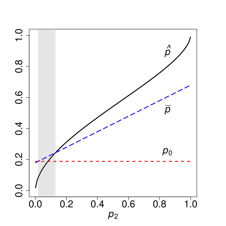
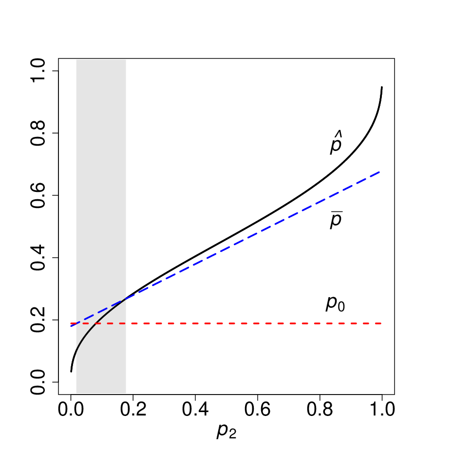
Figure 4 depicts the best approximate generalized probit ensemble as a function of the best base model’s forecasts, with the other two base models’ forecasts set to twice the base rate in their respective dataset. For these settings, the ensembles lie somewhere in between all weight on the best base model (xgboost) and equal weights on the base models. In each plot, we also highlight the anti-extremizing region in gray. In addition, because the estimated power parameters are high in these studies, we can see that the ensembles are nearly linear over much of the domain of $p_{\mathit{XGB}}$.

By Bernardo and Smith (2000, Prop. 5.5), expert $i$’s forecast of $x$ given $\boldsymbol{x}_{i}$ is given by

where $t_{i}=\sum_{j=N_{i-1}+1}^{N_{i}}h(x_{j})$ is the sufficient statistic for $\boldsymbol{x}_{i}$. Expert $i$’s forecast of $(y|\boldsymbol{x}_{i})$ is given by $P(y=1|\boldsymbol{x}_{i})=\int_{x\in A}f(x|\boldsymbol{x}_{i})\,dx$. Hence, $p_{i}=P(y=1|\boldsymbol{x}_{i})=F_{n_{i}}(\tau_{1}+t_{i})$. The decision maker, if he had direct access to the experts’ samples, would form the following forecast of $(y|\boldsymbol{x}_{1},\ldots,\boldsymbol{x}_{k})$:

The decision maker knows all the sample sizes because of the common knowledge assumption. The prior-predictive probability is given by

By the assumption that $F_{n}(t)$ is strictly monotonic in $t$, we can invert $F_{n}(t)$. By substitution according to $\tau_{1}=F_{0}^{-1}(p_{0})$ and $t_{i}=F_{n_{i}}^{-1}(p_{i})-\tau_{1}$ into (12), we have the result.

The Bernoulli distribution is a regular, one-parameter exponential family with pmf

where $a(x_{j})=1$, $b(\theta)=1-\theta$, $c(\theta)=\log(\frac{\theta}{1-\theta})$, and $h(x_{j})=x_{j}$. Its conjugate prior has the pdf

References

- Ahuja and Nash (1967) Ahuja, J C, S W Nash. 1967. The generalized Gompertz-Verhulst family of distributions. Sankhyā: The Indian Journal of Statistics, Series A 29(2) 141–156.
- Ariely et al. (2000) Ariely, D, W T Au, R H Bender, D V Budescu, C B Dietz, H Gu, T S Wallsten, G Zauberman. 2000. The effects of averaging subjective probability estimates between and within judges. Journal of Experimental Psychology Applied 6(2) 130–146.
- Baron et al. (2014) Baron, J, B A Mellers, P E Tetlock, E Stone, L H Ungar. 2014. Two reasons to make aggregated probability forecasts more extreme. Decision Analysis 11(2) 133–145.
- Bernardo and Smith (2000) Bernardo, J M, A F M Smith. 2000. Bayesian Theory. John Wiley & Sons, Ltd, Chichester, England.
- Box and Tiao (1973) Box, G E P, G C Tiao. 1973. Bayesian Inference in Statistical Inference. Adison-Wesley, Reading, MA.
- Breiman (1996) Breiman, L. 1996. Bagging predictors. Machine Learning 24(2) 123–140.
- Breiman (2001) Breiman, L. 2001. Random forests. Machine Learning 45(1) 5–32.
- Chen et al. (2004) Chen, K, L R Fine, B A Huberman. 2004. Eliminating public knowledge biases in information-aggregation mechanisms. Management Science 50 983––994.
- Chen and Guestrin (2016) Chen, T, C Guestrin. 2016. Xgboost: A scalable tree boosting system. Proceedings of the 22nd ACM SIGKDD International Conference on Knowledge Discovery and Data Mining. ACM, 785–794.
- Chipman et al. (2007) Chipman, Hugh A., Edward I. George, Robert E. Mcculloch. 2007. Bayesian ensemble learning. P B Schölkopf, J C Platt, T Hoffman, eds., Advances in Neural Information Processing Systems 19. MIT Press, Cambridge, MA, 265–272.
- Clemen (1987) Clemen, R T. 1987. Combining overlapping information. Management Science 33(3) 373–380.
- Clemen and Winkler (1986) Clemen, R T, R L Winkler. 1986. Combining economic forecasts. Journal of Business & Economic Statistics 4(1) 39–46.
- Dawid et al. (1995) Dawid, A P, M H DeGroot, J Mortera. 1995. Coherent combination of experts’ opinions. Test 4(2) 263–313.
- DeGroot (1974) DeGroot, M H. 1974. Reaching a consensus. Journal of the American Statistical Association 69(345) 118–121.
- DeGroot and Mortera (1991) DeGroot, M H, J Mortera. 1991. Optimal linear opinion pools. Management Science 37(5) 546–558.
- Džeroski and Ženko (2004) Džeroski, S, B Ženko. 2004. Is combining classifiers with stacking better than selecting the best one? Machine Learning 54(3) 255–273.
- Erev et al. (1994) Erev, I, T S Wallsten, D V Budescu. 1994. Simultaneous over-and underconfidence: The role of error in judgment processes. Psychological Review 101(3) 519–527.
- French (1980) French, S. 1980. Updating of belief in the light of someone else’s opinion. Journal of the Royal Statistical Society, Series A 143(1) 43–48.
- French (1986) French, S. 1986. Calibration and the expert problem. Management Science 32(3) 315–321.
- Friedman (2001) Friedman, J H. 2001. Greedy function approximation: A gradient boosting machine. Annals of Statistics 29(5) 1189–1232.
- Genest and Zidek (1986) Genest, C, J V Zidek. 1986. Combining probability distributions: A critique and an annotated bibliography. Statistical Science 1(1) 114–135.
- Gneiting and Raftery (2007) Gneiting, T, A E Raftery. 2007. Strictly proper scoring rules, prediction, and estimation. Journal of the American Statistical Association 102(477) 359–378.
- Hand and Till (2001) Hand, D J, R J Till. 2001. A simple generalisation of the area under the ROC curve for multiple class classification problems. Machine Learning 45(2) 171–186.
- Hastie and Tibshirani (1986) Hastie, T, R Tibshirani. 1986. Generalized additive models. Statistical Science 1(3) 297–318.
- Hora (2004) Hora, S C. 2004. Probability judgments for continuous quantities: Linear combinations and calibration. Management Science 50(5) 597–604.
- IARPA (2018) IARPA. 2018. Geopolitical forecasting challenge. https://www.iarpa.gov/challenges/gfchallenge.html.
- Karmarkar (1978) Karmarkar, U S. 1978. Subjectively weighted utility: A descriptive extension of the expected utility model. Organizational Behavior and Human Performance 21(1) 61–72.
- Kim et al. (2001) Kim, O, S C Lim, K W Shaw. 2001. The inefficiency of the mean analyst forecast as summary of forecast of earnings. Journal of Accounting Research 39 329–335.
- Larrick and Soll (2006) Larrick, R P, J B Soll. 2006. Intuitions about combining opinions: Misappreciation of the averaging principle. Management Science 52(1) 111–127.
- Lindley et al. (1979) Lindley, D V, A Tversky, R V Brown. 1979. On the reconciliation of probability assessments. Journal of the Royal Statistical Society, Series A 142(2) 146–180.
- Marinovic et al. (2013) Marinovic, I, M Ottaviani, P N Sorensen. 2013. Forecasters’ objectives and strategies. G Elliott, A Timmermann, eds., Handbook of Economic Forecasting, vol. 2. Elsevier, Amsterdam, Netherlands, 690–720.
- McConway (1981) McConway, K J. 1981. Marginalization and linear opinion pools. Journal of the American Statistical Association 76(374) 410–414.
- Mellers et al. (2014) Mellers, B, L Ungar, J Baron, J Ramos, B Gurcay, K Fincher, S E Scott, D Moore, P Atanasov, S A Swift, T Murray, E Stone, P E Tetlock. 2014. Psychological strategies for winning a geopolitical forecasting tournament. Psychological Science 25(5) 1106–1115.
- Mineo and Ruggieri (2005) Mineo, A M, M Ruggieri. 2005. A software tool for the exponential power distribution: The normalp package. Journal of Statistical Software 12(4) 1–24.
- Morris (1974) Morris, P A. 1974. Decision analysis expert use. Management Science 20(9) 1233–1241.
- Murphy and Winkler (1987) Murphy, A H, R L Winkler. 1987. A general framework for forecast verification. Monthly Weather Review 115(7) 1330–1338.
- Nelder and Wedderburn (1972) Nelder, J A, R W M Wedderburn. 1972. Generalized linear models. Journal of the Royal Statistical Society, Series A 135(3) 370–385.
- Raiffa and Schlaifer (1961) Raiffa, H, R Schlaifer. 1961. Applied Statistical Decision Theory. Harvard Business School, Boston, MA.
- Ranjan and Gneiting (2010) Ranjan, R, T Gneiting. 2010. Combining probability forecasts. Journal of the Royal Statistical Society: Series B (Statistical Methodology) 72(1) 71–91.
- Satopää et al. (2014) Satopää, V A, J Baron, D P Foster, B A Mellers, P E Tetlock, L H Ungar. 2014. Combining multiple probability predictions using a simple logit model. International Journal of Forecasting 30 344–356.
- Satopää et al. (2016) Satopää, V A, R Pemantle, L H Ungar. 2016. Modeling probability forecasts via information diversity. Journal of the American Statistical Association 111(516) 1623–1633.
- Shlomi and Wallsten (2010) Shlomi, Y, T S Wallsten. 2010. Subjective recalibration of advisors’ probability estimates. Psychonomic Bulletin & Review 17(4) 492–498.
- Smyth and Wolpert (1999) Smyth, P, D Wolpert. 1999. Linearly combining density estimators via stacking. Machine Learning 36(1-2) 59–83.
- Soury and Alouini (2015) Soury, H, M S Alouini. 2015. New results on the sum of two generalized Gaussian random variables. 2015 IEEE Global Conference on Signal and Information Processing (GlobalSIP). IEEE, 1017–1021.
- Stone (1961) Stone, M. 1961. The opinion pool. The Annals of Mathematical Statistics 32(4) 1339–1342.
- Subbotin (1923) Subbotin, M T. 1923. On the law of frequency of error. Matematicheskii Sbornik 31(2) 296–301.
- Tetlock and Gardner (2016) Tetlock, P, D Gardner. 2016. Superforecasting: The Art and Science of Prediction. Broadway Books, New York, NY.
- Tibshirani (1996) Tibshirani, R. 1996. Regression shrinkage and selection via the lasso. Journal of the Royal Statistical Society, Series B 58(1) 267–288.
- Turner et al. (2014) Turner, B M, M Steyvers, E C Merkle, D V Budescu, T S Wallsten. 2014. Forecast aggregation via recalibration. Machine Learning 95(3) 261–289.
- West and Harrison (1997) West, M, J Harrison. 1997. Bayesian Forecasting and Dynamic Models, 2nd ed.. Springer, New York, NY.
- Winkler (1968) Winkler, R L. 1968. The consensus of subjective probability distributions. Management Science 15(2) B61–B75.
- Winkler (1994) Winkler, R L. 1994. Evaluating probabilities: Asymmetric scoring rules. Management Science 40(11) 1395–1405.
- Winkler and Jose (2008) Winkler, R L, V R R Jose. 2008. Comments on: Assessing probabilistic forecasts of multivariate quantities, with an application to ensemble predictions of surface winds. Test 17 251––255.
- Winkler and Poses (1993) Winkler, R L, R M Poses. 1993. Evaluating and combining physicians’ probabilities of survival in an intensive care unit. Management Science 39(12) 1526–1543.
- Wolpert (1992) Wolpert, D H. 1992. Stacked generalization. Neural Networks 5(2) 241–259.
- Zhang et al. (2012) Zhang, Z, S Wang, D Liu, M I Jordan. 2012. EP-GIG priors and applications in Bayesian sparse learning. Journal of Machine Learning Research 13 2031–2061.