First-principles molecular transport calculation for the benzenedithiolate molecule

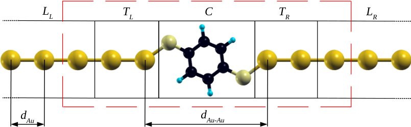
The system we are considering consists of a central region (C) attached to left and right leads, see figure 1. To determine the tight-binding (TB) parameters of the system we employ the pseudopotential plane-wave code Quantum Espresso [33]. The unit cell, red dashed line in figure 1, consists of the central region, left and right transition layers ($T_{L}$, $T_{R}$), also called buffer regions, and the surface part of the remaining leads ($L_{L}$,$L_{R}$). The size of the transition layers is chosen such that the electronic properties of the outermost atoms in the unit cell do not change anymore when the unit cell is increased. This ensures that the central region has negligible impact on the periodicity of the remaining leads [34, 35].

For all DFT calculations in this paper we have used the Perdew Zunger (PZ) exchange correlation functional within the local density approximation (LDA) and non-relativistic ultrasoft pseudopotentials from the Standard Solid-State Pseudopotentials (SSSP) library (PSlibrary 0.3.1) [37].

We have used Maximally Localized Wannier Functions (MLWF) [38, 39] to get localized orbitals and to set up the TB Hamiltonian [34, 35]. All Wannier transformations are done with wannier90 [40] which produces orthogonal MLWF. Therefore the derivation of the NEGF formalism in section 2.2 is demonstrated only for orthogonal bases. A derivation for non-orthogonal bases in the coherent regime can be found in [41]. In the localized basis the Hamilton operator of the unit cell is then given by

$${\mathop{\hat{H}}}=\left(\begin{array}[]{ccccc}{\mathop{\hat{H}}}_{L_{L}}&{\mathop{\hat{V}}}_{L_{L}T_{L}}&&&{\mathop{\hat{V}}}_{L_{L}L_{R}}\\ {\mathop{\hat{V}}}_{L_{L}T_{L}}^{\dagger}&{\mathop{\hat{H}}}_{T_{L}}&{\mathop{\hat{V}}}_{T_{L}C}&\\ &{\mathop{\hat{V}}}_{T_{L}C}^{\dagger}&{\mathop{\hat{H}}}_{C}&{\mathop{\hat{V}}}_{CT_{R}}&\\ &&{\mathop{\hat{V}}}_{CT_{R}}^{\dagger}&{\mathop{\hat{H}}}_{T_{R}}&{\mathop{\hat{V}}}_{T_{R}L_{R}}\\ {\mathop{\hat{V}}}_{L_{L}L_{R}}^{\dagger}&&&{\mathop{\hat{V}}}_{T_{R}L_{R}}^{\dagger}&{\mathop{\hat{H}}}_{L_{R}}\\ \end{array}\right)\;.$$

(3)

The outermost atoms of the unit cell are periodically continued and form the non-interacting leads ($L_{L}$, $L_{R}$) in the TB model. In this way we determine all single-particle parameters of the Hamiltonian.

We describe the electron-electron interaction by an extended Hubbard Hamiltonian in the central region, which has the form

$${\mathop{\hat{H}}}_{C}={\mathop{\hat{H}}}_{0}+{\mathop{\hat{H}}}_{1}$$

(4)

where ${\mathop{\hat{H}}}_{0}$ is the single-particle part and ${\mathop{\hat{H}}}_{1}$ the interaction part of the model Hamiltonian. We neglect correlation effects in the leads ($L_{L}$,$T_{L}$,$L_{R}$,$T_{R}$) and we expect correlation effects to be important only in the central region, because on the molecule the wave functions are more localized. The single-particle part of the model Hamiltonian in the central region in second quantization is given by

$${\mathop{\hat{H}}}_{0}=\sum_{ij}^{N}\tilde{t}_{ij}{{\mathop{\hat{a}_{i}^{\dagger}}}}{\mathop{\hat{a}}}_{j}\;.$$

(5)

The indices $i=\{\bar{i},\sigma\}$ and $j=\{\bar{j},\sigma^{\prime}\}$ include the wave function indices $\bar{i}$ and $\bar{j}$ and the spins $\sigma$ and $\sigma^{\prime}$. The operator ${{\mathop{\hat{a}_{i}^{\dagger}}}}$ creates an electron on orbital $\Psi_{i}({\bf r})$ which we obtain by the MLWF construction. The hopping parameters $\tilde{t}_{ij}$ are

$$\tilde{t}_{ij}=\{QEQ^{\dagger}\}_{\bar{i}{\bar{j}}}\;,$$

(6)

where $Q$ is the matrix which diagonalizes the TB Hamiltonian and $E$ are the corresponding eigenenergies. The interaction part of the model Hamiltonian is given by

$${\mathop{\hat{H}}}_{1}=\frac{1}{2}\sum_{i\neq j}^{N}U_{ij}{\mathop{\hat{n}}}_{i}{\mathop{\hat{n}}}_{j}\;.$$

(7)

The density-density term form of the Hubbard model is only justified if the non-density-density term is small which also requires that the orbitals are maximally localized. The interaction parameters $U_{ij}$ are calculated via

$$U_{ij}=\int d^{3}r\int d^{3}r^{\prime}\left|\Psi_{i}({\bf r})\right|^{2}\left|\Psi_{j}({\bf r^{\prime}})\right|^{2}U({\bf r},{\bf r^{\prime}})$$

(8)

with the screened Coulomb potential

$$U({\bf r},{\bf r^{\prime}})=\frac{1}{4\pi\epsilon_{0}\eta|{\bf r}-{\bf r^{\prime}}|}$$

(9)

where $\eta$ is the screening. According to [19] we set the screening to be constant. The Random Phase Approximation (RPA) [42] would be a possibility to determine the screening consistently.

The electron correlations already included in DFT, have to be subtracted in order to avoid double counting. Here we choose the around mean-field approximation (AMF) [43], because it generally gives good results for weakly correlated systems. That is, we have subtracted the Hartree term $\Delta t_{\bar{i}\bar{i}}$ of the interaction part from the bare hopping $\tilde{t}_{ij}$. This approach is justified as follows. If we apply the LDA approximation to the model Hamiltonian we end up with the same band structure as that is obtained from the original band structure calculation. The double counting correction leads to modified hopping parameters $\tilde{t}_{ij}\to t^{C}_{ij}$ with

$$t_{\bar{i}{\bar{j}}}^{C}=\tilde{t}_{\bar{i}{\bar{j}}}-\Delta t_{\bar{i}\bar{i}}\delta_{\bar{i}{\bar{j}}}\;.$$

(10)

The Hartree term is given by

	$\displaystyle\Delta t_{\bar{i}\bar{i}}$	$\displaystyle\approx U_{\bar{i}\bar{i}}n_{\bar{i}}^{0}+\sum_{{\bar{m}}\neq\bar{i}}2U_{\bar{i}{\bar{m}}}n_{\bar{m}}^{0}$			(11)
		$\displaystyle=\sum_{\bar{k}}^{N_{occ}}\sum_{\bar{m}}\left|\{Q^{\dagger}\}_{{\bar{k}}{\bar{m}}}\right|^{2}\left(U_{\bar{i}\bar{i}}\delta_{\bar{i}{\bar{m}}}+2U_{\bar{i}{\bar{m}}}(1-\delta_{\bar{i}{\bar{m}}})\right)$

where $n_{\bar{i}}^{0}$ is the equilibrium population of the $i$-th orbital obtained in the DFT calculation. The model Hamiltonian for the central region has finally the form

$${\mathop{\hat{H}}}_{C}=\sum_{ij}^{N}t^{C}_{ij}{{\mathop{\hat{a}_{i}^{\dagger}}}}{\mathop{\hat{a}}}_{j}+\frac{1}{2}\sum_{i\neq j}^{N}U_{ij}{\mathop{\hat{n}}}_{i}{\mathop{\hat{n}}}_{j}\;.$$

(12)

The full self-consistent non-equilibrium transport calculation could be done by feeding the non-equilibrium potential, obtained from the non-equilibrium densities in the transport calculation, back into DFT and repeat this procedure until self-consistency is reached [44, 45, 46].

We have used the Keldysh formalism [47] to compute the current through the central region. In steady-state the two-time Green’s function depends only on the time difference and can be treated efficiently in frequency space. The steady-state current from the left transition layer to the central region can be calculated by integrating over the real part of the Keldysh Green’s function

$$I=\frac{e}{h}\int_{-\infty}^{\infty}d\omega\sum_{\begin{array}[]{c}i\in T_{L}\\ j\in C\end{array}}\Re\left(V_{ij}\mathcal{G}^{k}_{ij}(\omega)\right)\;.$$

(13)

Here, $i$ and $j$ denote the orbitals within the clusters $T_{L}$ and $C$, see figure 1, for calculating the current between the left transition layer and the central region. In this paper we employ non-equilibrium cluster perturbation theory (n-CPT) [48, 9] to compute the Keldysh Green’s function $\mathcal{G}$ of the interacting non-equilibrium system required in (13). Within n-CPT, (13) reduces to the well-known Landauer-Büttiker formula [49].

$$I=\frac{e}{h}\int_{-\infty}^{\infty}d\omega\left(f_{R}(\omega)-f_{L}(\omega)\right)T(\omega)$$

(14)

$T(\omega)$ denotes the transmission function

$$T(\omega)=\Tr\left({\bf\Gamma}_{L}\bm{\mathcal{G}}^{r}_{CC}{\bf\Gamma}_{R}\bm{\mathcal{G}}^{a}_{CC}\right)\;,$$

(15)

where ${\bm{\Gamma}}_{\nu}$ with $\nu\in\{L,R\}$ is the anti-hermitian part of the hybridization function

$${\bm{\Delta}}^{r}_{\nu}={\bf R}_{\nu}-\frac{i}{2}{\bm{\Gamma}}_{\nu}\;.$$

(16)

We denote matrices with bold faced letters and for simplicity of the notation, we have omitted the $\omega$ arguments. To this end, the entire system is decomposed into the device ($C$), e.g. the BDT molecule, and the two leads, which are further decomposed into $L_{L}$ plus $T_{L}$ on the left side and $L_{R}$ plus $T_{R}$ on the right. We calculate the full Green’s function for indices of the central region ${\bm{\mathcal{G}}}_{CC}$ within the CPT approximation, i.e. we use the following Dyson equation

	$\displaystyle\big(\bm{{\mathcal{G}}}_{CC}^{r,a}\big)^{-1}$	$\displaystyle=\big({\bf g}_{CC}^{r,a}\big)^{-1}-\sum_{\nu\in\{L,R\}}\underbrace{{\bf V}_{CT_{\nu}}{\bf G}_{T_{\nu}T_{\nu}}^{r,a}{\bf V}_{T_{\nu}C}}_{{\bf\Delta}_{\nu}^{r,a}}$			(17)
		$\displaystyle=\big({\bf g}_{CC,0}^{r,a}\big)^{-1}-{\bf\Sigma}^{r,a}-\sum_{\nu\in\{L,R\}}{\bf\Delta}_{\nu}^{r,a}\;.$

In CPT the Green’s function ${\bf g}^{r,a}_{CC}$ of the isolated central cluster is required. From the Dyson equation

$$\big({\bf g}^{r,a}_{CC}\big)^{-1}=\big({\bf g}^{r,a}_{CC,0}\big)^{-1}-{\bm{\Sigma}}^{r,a}$$

(18)

it is clear that in the interacting case, the CPT approximation is equivalent to approximating the self-energy by that of the isolated cluster. Therefore it is important to cut the system in a way that the coupling between the transition layers and the central region is weak compared to the hopping parameters within the central region. The Green’s function of the isolated central cluster can be calculated using the Lehmann representation

	$\displaystyle\left\{{\bf g}^{r}_{CC}\right\}_{ij}=$	$\displaystyle\bra{\Omega}{\mathop{\hat{a}}}_{i}\frac{1}{\omega+i0^{+}-{\mathop{\hat{H}}}_{C}+E_{0}}{{\mathop{\hat{a}_{j}^{\dagger}}}}\ket{\Omega}$			(19)
		$\displaystyle+\bra{\Omega}{{\mathop{\hat{a}_{j}^{\dagger}}}}\frac{1}{\omega+i0^{+}+{\mathop{\hat{H}}}_{C}-E_{0}}{\mathop{\hat{a}}}_{i}\ket{\Omega}\;.$

If the system is not too far away from the equilibrium situation, it will still be a good approximation to consider only excitations from the ground state to higher states and hence the corresponding self-energy.

The Green’s function of the isolated left lead with indices restricted to the transition region ${\bf G}_{T_{L}T_{L}}$ is needed in (17). We will also need ${\bf G}_{T_{R}T_{R}}$. To calculate ${\bf G}_{T_{\nu}T_{\nu}}$ for $\nu\in\{L,R\}$ we once more introduce a cluster decomposition of the leads into part $L_{\nu}$ and $T_{\nu}$, introduced before. The exact Dyson equation for this decomposition yields

$$\left({\bf G}_{T_{\nu}T_{\nu}}\right)^{-1}=\left({\bf g}_{T_{\nu}T_{\nu}}\right)^{-1}-{\bf V}_{T_{\nu}L_{\nu}}\;{\bf g}_{L_{\nu}L_{\nu}}\;{\bf V}_{L_{\nu}T_{\nu}}.$$

(20)

where ${\bf g}_{T_{L}T_{L}}$ stands for the Green’s function of the isolated transition region, which can be computed easily, as the matrix dimension is small. ${\bf g}_{L_{\nu}L_{\nu}}$ on the other hand represents the Green’s function of the isolated semi-infinite part $L_{\nu}$ of lead $\nu$ that is composed of identical unit cells. The hopping elements ${\bf V}_{T_{\nu},L_{\nu}}$ couple only to the unit cell near to the transition region in each lead and therefore only the surface part of ${\bf g}_{L_{\nu}L_{\nu}}$ is required, which can be determined iteratively by using the method of Sancho et al. [50]. An alternative technique for calculating the hybridization function is to use complex absorbing potentials [51].

A bias voltage $V_{b}$ drives the system out of equilibrium and enters the calculation as a shift of the on-site energies and the chemical potential by $-V_{b}/2$ for the left lead and by $+V_{b}/2$ for the right lead. In the Landauer-Büttiker formula $V_{b}$ enters also in the Fermi functions. A gate voltage $V_{g}$ can be applied by shifting the on-site energies of $\tilde{t}_{\bar{i}{\bar{j}}}$.

The spectral density and the conductivity are important quantities for our analyses and they are defined as

	$\displaystyle A_{\nu\nu}(\omega)$	$\displaystyle=-\frac{1}{\pi}\Im\Tr\left({\bf g}^{r}_{\nu\nu}(\omega)\right)$			(21)
	$\displaystyle G$	$\displaystyle=\frac{dI}{dV_{b}}\;.$			(22)

In a first step we have applied the DFT+NEGF formalism to a system consisting of a BDT molecule sandwiched between two gold chains, schematically drawn in figure 1. As shown below in the case of monoatomic gold chains it is possible to include all lead atoms in the Wannier transformation in a controlled way. In mechanically controllable break junctions (MCBJ) or with an scanning tunnelling microscope (STM) the formation of monoatomic gold chains was demonstrated under elongation of the junction by several authors [52, 44, 53, 54, 55]. In a first step we have performed DFT calculations ¹¹ 1 We used a cut-off energy for the wavefunction of $E_{\rm cowf}=64~$Ry and the charge density of $E_{con}=512~$Ry, the Methfessel-Paxton smearing technique with the smearing parameter $E_{\rm tsm}=0.01~$Ry, the vacuum distance $d_{\rm vac}=12~$Å  and $32$ k-points. for the periodic chain of monoatomic gold atoms. All the parameters are converged with respect to the total energy within $5~$meV. In order to find the equilibrium geometry, we have calculated the total energy of the chain for different distances $d_{Au}$ between the gold atoms. We find an optimal distance of $d_{Au}=2.515~$Å  which is close to the LDA result $2.51~$Å  in [56].

The band structure of the Au chain in an interval around $E_{F}$ is shown in the left panel of figure 2. The $\Gamma$-$X$ axis is always the axis along the gold chain in reciprocal space. The 6p bands are at higher energies. The 6s and 5d bands coincide exactly with the Wannier bands, which demonstrates the properness of the Wannier transformation. The dotted lines represent the inner and the outer energy window needed to disentangle the 6s and 5d bands from the 6p band in the Wannier transformation. In figure 2 tight binding (TB1) means that only hopping processes to nearest neighbour gold atoms are taken into account. The 6s band and the 5d bands separate into the two bands corresponding to the $d_{xz}$ and the $d_{yz}$ orbital (Channel 1) and four bands corresponding to orbitals with inversion symmetry with respect to the $xy$-plane (Channel 2). The definition of the coordinate system is according to figure 5. Each symmetry channel will only couple to orbitals of the same symmetry and therefore transport takes place in two separated channels. The TB1 approximation turns out to be a good approximation for the channel 1 bands, which are mainly interesting for transport. The right panel of figure 2 is the calculated equilibrium ($V_{b}=0$) transmission function for TB1 and is similar to the results obtained in [56]. In the coherent regime the transmission function is proportional to the number of bands at a certain energy.

After having calculated the Hamiltonian of the monoatomic Au chain, we considered the full system, including BDT ²² 2 We used a cut-off energy for the wavefunction of $E_{\rm cowf}=100~$Ry and the charge density of $E_{con}=400~$Ry, the Methfessel-Paxton smearing technique with the smearing parameter $E_{\rm sm}=0.001~$Ry, the vacuum distance $d_{\rm vac}=18~$Å  and $1$ k-point.. The BDT molecule can assume different geometry configurations between the two semi-infinite gold chains. In the line configuration the BDT molecule is forced to be on the gold chain axis. In the atop configuration the BDT molecule slightly hops out of the gold chain axis, while it twists out of the axis in the twisted configuration as shown in figure 1. There are also mixed configurations between atop and twisted, called atop-twisted and twisted-twisted. In order to determine the energetically favourable configuration, we compute the total energy as function of the distance between the gold atoms near to the BDT molecule $d_{Au-Au}$, namely the gap between the two (left and right) semi-infinite gold chains, for different configurations, see figure 1 and 3. The distance between the gold atoms was fixed $d_{Au}$ during the geometry optimizations.

At $d_{Au-Au}\approx 8.1$ the BDT molecule rearranges into thienothiophene. It occurs that the twisted configuration of the BDT atom is energetically most favoured and, consequently, we have chosen this configuration for the ensuing transport calculations. The optimized distance is $d_{Au-Au}=9.16~$Å. We have chosen 6 gold atoms per unit cell, which ensures that the eigenvalues of the atoms at the outer edges of the unit cell (see figure 1) are converged. We have chosen the size such that the changes in eigenenergies are less than $0.05~$eV.

The left panel in figure 4 depicts a comparison of the band structure obtained with the full plane wave basis and with the Wannier basis. The Wannier transformation is performed only at the $\Gamma$-point. In the Wannier transformation we picked out 47 bands, 35 corresponding to the 6 gold atoms and there are 12 BDT bands within this energy range. At the $\Gamma$-point the PWSCF bands coincide exactly with the Wannier levels, which demonstrates again the properness of the Wannier transformation. The obtained Wannier basis functions of the gold atoms coincide with the Wannier basis functions of the pure gold chain, which shows that the disentanglement procedure of the 6s and 5d bands from the 6p bands is done correct. Projections of the wavefunctions onto orthogonalized atomic wavefunctions show whether the Wannier levels belong to the gold leads and the transition layers or to the BDT molecule. The right panel presents the eigenlevels of the decoupled BDT molecule, the eigenenergies of ${\mathop{\hat{H}}}_{C}$. As mentioned above and outlined in [6, 29] transport takes place in separated channels. Channel 1 (blue dashed) consists of $p_{z}$-like BDT orbitals and channel 2 (cyan) of $p_{xy}$-like BDT orbitals. Each channel couples only to the corresponding channel in the gold leads.

The eigenorbitals of channel 1 are shown in figure 5. The shape of the orbitals can be explained by the symmetry of the benzene molecule, which has the point group $D_{6h}$. LUMO+2 is the $B_{2g}$-orbital, LUMO+1 and LUMO are the $E_{2u}$-orbitals, HOMO-4 is the $A_{2u}$-orbital and the others are a mixture of the benzene $E_{1g}$- and the sulfur $p_{z}$-orbitals.

Due to the fact that only the HOMO level is close to the Fermi energy it is the level mainly contributing to transport which is in general the case in systems with thiol-anchoring groups [58]. The HOMO orbital is an unsaturated sulfur $p$-orbital and can also be compared to [59, 31]. Passivating the unsaturated sulfur $p$-orbitals would shift the HOMO level away from the Fermi energy and produce lower conductances [16]. Charge transport through channel 1 is blocked due to the fact that there are no empty states with $p_{z}$-like symmetry in the monoatomic gold chain (only a $sd$-hybridized orbital belonging to channel 2 is above the Fermi level in figure 2). The levels corresponding to channel 2 are more than $2~$eV below the Fermi energy. Therefore, transport in this channel is due to the broadening of the leads and the current-voltage characteristic nearly linear. The conductivity for the BDT molecule connected with monoatomic Au chains is almost constant and in the order of $0.01~G_{0}$ for biasvoltages bellow $4~$V which is in the order of the experimental values of $0.01~G_{0}$ [23, 24, 25, 26]. But using gold tips or bulk-like gold as leads [29, 6] produces empty states with $p_{z}$-like symmetry and activates channel 1 which raises the conductance. Therefore the theoretical LDA result for the Au-BDT-Au system with bulk-like leads is $0.28~G_{0}$ [16].

Since channel 1 contains the HOMO-orbital and the typical benzene $p_{z}$ orbitals it would be the most important channel if supported by the leads. The coupling between leads and the channels depends on the geometry of the junction and therefore as mentioned above gold tips or bulk-like gold as leads [29, 6] activate channel 1. Also the use of platinum instead of gold opens channel 1 because platinum has one electron less than gold and therefore also orbitals with $p_{z}$-like symmetry contribute to transport.

In order to activate channel 1 we have replaced the gold atoms by platinum ones in our calculations ³³ 3 We used a cut-off energy for the wavefunction of $E_{cowf}=60~$Ry and the charge density of $E_{con}=200~$Ry, the Methfessel-Paxton smearing technique with the smearing parameter $E_{sm}=0.005~$Ry, the vacuum distance $d_{vac}=12~$Å  and $60$ k-points.. The optimized distance between the platinum atoms $d_{Pt}=2.328~$Å  is comparable to the value of $2.34~$Å  in [60]. The plane-wave pseudopotential band structure, Wannier bands and TB1 bands along with the transmission function are shown in figure 6. In the Pt chain not just channel 2 but also channel 1 bands contribute to the equilibrium transmission at the Fermi energy.

We now consider the Pt-BDT-Pt system ⁴⁴ 4 We used a cut-off energy for the wavefunction of $E_{cowf}=80~$Ry and the charge density of $E_{con}=320~$Ry, the Methfessel-Paxton smearing technique with the smearing parameter $E_{sm}=0.005~$Ry, the vacuum distance $d_{vac}=15~$Å  and $1$ k-point..

The optimized distance between the Pt atoms near to the BDT molecule is $d_{Pt-Pt}=8.58~$Å. It is necessary to take at least 8 platinum atoms per unit cell to ensure that the influence of the BDT molecule on the lead platinum atoms is negligible. The comparison of the PW band structure with the Wannier bands is given in the left panel of figure 7. In the Wannier transformation we retained 62 bands, 47 corresponding to the 8 platinum atoms and there are 15 BDT bands within this energy range. The right panel presents the decoupled levels of the BDT molecule and is comparable to figure 4 disregarding 3 more levels in channel 2 needed to get all the platinum levels in the calculation. In the following we will only discuss channel 1 because due to the level alignment the current in channel 2 is an order of magnitude smaller. The orbitals of channel 1 look similar to the ones in the Au-BDT-Au calculation in figure 5. The orbitals in figure 8 are the localized Wannier orbitals of the BDT molecule in the Pt-BDT-Pt calculation. These are the 8 orbitals entering the TB model for the central region. They all have $p_{z}$ symmetry.

The matrix form of the TB Hamiltonian of the central region, in the basis of the localized orbitals in figure 8, and the coupling matrices to the leads that have been used in the calculations are given in section A. The Fermi energy in the transport Hamiltonian is adjusted such that the local DOS of channel 1 of the atom further away from the BDT molecule has the same filling as in the pure atom chain.

The plot in the middle of figure 9 shows the spectral density $A_{CC}(\omega)$ of the isolated central cluster, namely the isolated BDT molecule. The curves labelled by DFT+CPT represent the result for the correlated system, which will be explained in section 3.4. The peaks in the DFT+NEGF result are at $-0.4~$eV, $-2.0~$eV and $-2.3~$eV. As discussed above the HOMO level closer to the Fermi level ($-0.4~$eV) is mainly responsible for the transport.

The spectral density at the surface atom of the left and the right lead is shown in the left and the right panel of figure 9. The spectral density of a homogeneous multiorbital chain is a superposition of semi-circles, see $A_{LL}(\omega)$ and $A_{RR}(\omega)$. Coupling the homogeneous chains to the the transition layers changes the semi-circular structure of the spectral density. The spectral densities $A_{TLi}(\omega)$ and $A_{TRi}(\omega)$ are located $i$ atoms away from the last point of the transition region, i.e. points with larger $i$ are closer to the central regions. We nicely see, how the spectral function gradually changes from the multi-circular structure of the homogeneous chain to the structure of the spectral densities $A_{TL3}(\omega)$ and $A_{TR3}(\omega)$, which consists of peaks at $-1.6$ and $-0.5$ and a spike at about $-1.3$. The grey shaded area indicates the filling. The remarkable point is that the spectral function of the transition region, that enters the transmission function and therefore the current, has a complex structure that will even change when a voltage is applied. As demonstrated by Cuniberti et al. [61, 4] low dimensional leads can affect the conductance due to the finite band width and the structure in the DOS. If the DOS is nearly constant one can use the wide-band limit (WBL) approximation which works well for systems with bulk metal electrodes [62]. However the DOS of a one-dimensional chain has Van Hove singularities near the band edge and the WBL approximation does not work. The key message therefore is that the details of the leads in such a molecular device are of crucial importance for the transport properties. This adds to the observation that the symmetry of the molecular orbitals and the leads can lead to selection rules as far as transport channels are concerned.

Next we present various aspects of the charge stability of the Pt-BDT-Pt system. The stability diagram computed with the DFT+NEGF formalism is presented in figure 10. We have restricted the bias voltage to $-3~$V$<V_{b}<3~$V, because otherwise we would have to include platinum $p$-orbitals, and likewise we have restricted the gate voltage to the interval $-2~$V$<V_{g}<2~$V, otherwise channel 2 becomes important. All diagrams are calculated at an inverse lead temperature of $\beta=300~1/$eV, which enters in the Fermi functions of the leads. The conductance at $V_{b}=V_{g}=0$ is $0.52~G_{0}$ and is considerable higher than the experimental ($0.01~G_{0}$ [23, 24, 25, 26]) and theoretical LDA ($0.28~G_{0}$ [16]) values of Au-BDT-Au systems. Beside the influence of the different contact material the formation of monoatomic chains results in large increases in the conductance [31, 52, 63]. The distance $d_{Pt-Pt}$ is also small compared to experimental values, where the monoatomic chains arise under applying stress to the leads. This results in a higher coupling strength between the leads and the central region.

Most strikingly, the stability diagram in figure 10 does not show the usual structure of crossing straight lines, resulting in rhombic patterns. The only such structure is the pair of straight lines starting at the left edge of the diagram with $V_{g}=0.8$ and $V_{g}=1.3$, respectively. They correspond to the level at $-2.3~$eV. At $V_{b}=3$ the Fermi energy of the right leads is shifted to $\mu=-1.5$. Above the Fermi level the remaining DOS of unoccupied states has a width of $\Delta E_{empty}=0.5$ eV, see figure 9. Hence, the transport window of the right lead is $(-1.5,-1.0)$ eV. With $V_{g}=0.8$ the level, which was originally at $-2.3$ eV is shifted to the lower edge of the transport window and with $V_{g}=1.3$ it is shifted to the upper edge. This constant distance between the lines is an effect of the band edge according to which a positive conductance is always followed by a negative one. In our case the distance between the lines along the $V_{b}$-axis is $\Delta V_{b}=2\Delta E_{empty}=1~$eV. The factor two results from the fact that half of the bias voltage is applied to each lead. The slope of the lines is constant and equal to $\pm 1/2$. If the leads are shifted with $\pm V_{b}/2$, one needs $2V_{b}$ to compensate a shift in $V_{g}$. As a consequence of weak coupling of this level to the leads the effects can be seen so clearly.

The levels at $-2.0~$eV and $-0.4~$eV produce a similar structure but at different energies. The structure can be explained by a ”band edge effect” and a ”supporting effect”. To explain the ”supporting effect” we have projected out the level at $-0.4~$eV. The resulting charge stability diagram is depicted in figure 11. Comparison to the full calculation illustrates that in a broad range of $V_{g}$ it is enough to use a single-level model for describing the transport through the BDT molecule and suggests approaches based on a single-level model [64].

The structure in the stability diagram is a consequence of the strong coupling to the leads. In the present case the leads within channel 1 consist again of two nearly decoupled channels, the ”supporting channel” and the ”conducting channel”. The real (imaginary) part $R^{L}$ ($\Gamma^{L}$) of the retarded left lead hybridization function $\Delta^{L,r}$ for these two channels are shown in figure 12.

Only the ”conducting channel” has states above the Fermi level. The real part $R^{L}$ shifts the levels in the central region. $R^{L}$ of the ”supporting channel” has anti-resonances at $\omega_{1}=-0.5~$eV and $\omega_{2}=-1.6~$eV. The spike at $-1.3~$eV is due to the small coupling between the channels in the leads and its influence is negligible. The imaginary part $\Gamma^{L}$ broadens all the levels and has maxima at the anti-resonances in $R^{L}$. By the ”supporting effect” we mean that at every $V_{b}$, where the positive branch of an antiresonance of $R_{L}$ hits the transport window of the opposite lead, the energy level in the central region will be shifted up to higher energies and therefore one needs smaller $V_{g}$ to compensate this and the conductivity structure in the stability diagram bends down, see figure 11. The blue dashed lines show the case where the positive branches of the anti-resonances of $R_{L}$ hit the upper edge of the opposite lead,

	$\displaystyle\omega_{1}-\frac{V_{b}}{2}$	$\displaystyle=\Delta E_{empty}+\frac{V_{b}}{2}$			(23)
	$\displaystyle\omega_{2}-\frac{V_{b}}{2}$	$\displaystyle=\Delta E_{empty}+\frac{V_{b}}{2}\;,$			(24)

and act as limit where the effect is maximal. The same effect with opposite sign happens if a negative branch of an antiresonance of $R_{L}$ hits the transport window of the opposite lead, there the conductivity structure in the stability diagram bends up. The red dashed line in figure 11 shows the case where the negative branch of the anti-resonances of $R_{L}$ hits the lower edge of the transport window, the Fermi energy, of the opposite lead,

$$\omega_{2}-\frac{V_{b}}{2}=+\frac{V_{b}}{2}\;.$$

(25)

There the structure in the stability diagram is maximally bent up. This effect explains the appearance of more than one maximum in the current voltage characteristic even if there is only a single level in the central region.

Between $-\Delta E_{empty}<V_{b}<\Delta E_{empty}$ is the usual structure of a stability diagram, but smeared out due to the coupling of the leads. Disabling the supporting channel produces the stability diagram in figure 13 where the structure can be explained just by the ”band edge effect”.

After having discussed the properties of the single-particle part of the Hamiltonian, we now include many-body effects using the DFT+CPT method. The interaction parameters $U_{ij}$ entering the model Hamiltonian in (12) are determined by numerical integration of (8) and listed in section A. We take a constant screening parameter $\eta=1.5$ as proposed by Ryndyk et al. [19]. The values obtained in our calculation for the nearest neighbour hopping between the carbon atoms within benzene in (27) and the on-site Hubbard interaction in (29) are comparable to those reported in [65].

In table 1 the lowest many-body eigenenergies of the isolated central region are listed. The ground state ($10_{g}$) is in the $10$-particle sector and is a singlet state. The other low-lying states in the $10$-particle sector have singlet or triplet symmetry. The lowest eigenenergies in the $9$-particle sector are doublet states.

Including interaction in principle shifts levels and spectral weight away from the Fermi energy and produces additional peaks and therefore signatures in the current-voltage characteristic at higher voltages. Therefore the benzene band gap increases compared to the LDA calculation [66] and can cause a reduction of the current. As suggested by [3, 32] the gap also widens in calculations based on the self-interaction correction (SIC) in DFT. In our transport system adding the full interaction the HOMO level is shifted down to $-0.6~$eV, see DFT+CPT result in figure 9. The peaks obtained by this calculation can be identified with excitations obtained by a true many-body calculation for the effective Hubbard model. There is a peak at $-0.6~$eV corresponding to the excitation from the $10_{g}$ to the $9_{g}$ state. The next peak is at $-2.1~$eV and corresponds to the excitation from the $10_{g}$ to the $9^{\prime}$ state. This excitation needs more energy than we have taken into account in our Wannier basis and are therefore negligible.

The stability diagram obtained by including electron-electron correlations within CPT does not change qualitatively for $V_{g}<0.6~$eV, see figure 14. The drastic change at $V_{g}=0.6~$eV is an artefact of CPT. Equation (19) is solved once for each $V_{g}$ independent of the applied $V_{b}$. At $V_{g}=0.6~$eV the HOMO level gets depleted and therefore the particle sector changes. We expect that using more sophisticated non-equilibrium approaches like the ME+CPT calculation [20] the drastic change at $V_{g}=0.6~$eV should disappear. The conductance at $V_{b}=V_{g}=0$ of $0.86~G_{0}$ is higher than the result obtained with LDA even though the HOMO is shifted down in energy and has less spectral weight. In the DFT+CPT calculation the spectral weight on the HOMO level is lower but distributed in a way that there is more weight in the orbitals near to the leads which causes the higher conductance. Thygesen et al. [16] have obtained the same trend at the BDT molecule connected with gold tips and studied with LDA and GW.

In contrast to Ryndyk et al. [19] the lead coupling effects overcome the influence of strong electron correlations in our transport system because of stronger coupling between leads and BDT due to the geometry of the transport system.

References

- [1] Joachim C and Ratner M A 2005 PNAS 102 8801
- [2] Cuevas J C and Scheer E 2010 Molecular electronics: an introduction to theory and experiment vol 1 (World Scientific)
- [3] Pontes R B, Rocha A R, Sanvito S, Fazzio A and da Silva A J R 2011 ACS Nano 5 795–804
- [4] Cuniberti G, Großmann F and Gutiérrez R 2002 The Role of Contacts in Molecular Electronics Advances in Solid State Physics vol 42
- [5] Kim Y, Hellmuth T J, Bürkle M, Pauly F and Scheer E 2011 ACS Nano 5 4104–4111
- [6] Di Ventra M, Pantelides S T and Lang N D 2000 Phys. Rev. Lett. 84 979–982
- [7] Khomyakov P A and Brocks G 2004 Phys. Rev. B 70 195402
- [8] Balzer M and Potthoff M 2011 Phys. Rev. B 83 195132
- [9] Nuss M, Heil C, Ganahl M, Knap M, Evertz H G, Arrigoni E and von der Linden W 2012 Phys. Rev. B 86 245119
- [10] Knap M, von der Linden W and Arrigoni E 2011 Phys. Rev. B 84 115145
- [11] Breuer H and Petruccione F 2007 The Theory of Open Quantum Systems (Oxford University Press)
- [12] Arrigoni E, Knap M and von der Linden W 2013 Phys. Rev. Lett. 110 086403
- [13] Dorda A, Nuss M, von der Linden W and Arrigoni E 2014 Phys. Rev. B 89 165105
- [14] Dorda A, Ganahl M, Evertz H G, von der Linden W and Arrigoni E 2015 Phys. Rev. B 92 125145
- [15] Hedin L 1965 Phys. Rev. 139 A796–A823
- [16] Strange M, Rostgaard C, Häkkinen H and Thygesen K S 2011 Phys. Rev. B 83 115108
- [17] Thygesen K S and Rubio A 2008 Phys. Rev. B 77 115333
- [18] Jacob D 2015 Journal of Physics: Condensed Matter 27 245606
- [19] Ryndyk D A, Donarini A, Grifoni M and Richter K 2013 Phys. Rev. B 88 085404
- [20] Nuss M, Dorn G, Dorda A, von der Linden W and Arrigoni E 2015 Phys. Rev. B 92 125128
- [21] Reed M A, Zhou C, Muller C J, Burgin T P and Tour J M 1997 Science 278 252–254
- [22] Lörtscher E, Weber H B and Riel H 2007 Phys. Rev. Lett. 98 176807
- [23] Song H, Kim Y, Jang Y H, Jeon g H, Reed M A and Takhee L 2009 Nature 462 1039–1043
- [24] Xiao X, Xu B and Tao N J 2004 Nano Letters 4 267–271
- [25] Tsutsui M, Taniguchi M and Kawai T 2009 Nano Letters 9 2433–2439
- [26] Kiguchi M, Nakamura H, Takahashi Y, Takahashi T and Ohto T 2010 The Journal of Physical Chemistry C 114 22254–22261
- [27] Xie Z, Baldea I, Smith C E, Wu Y and Frisbie C D 2015 ACS Nano 9 8022–8036
- [28] Kim Y, Pietsch T, Erbe A, Belzig W and Scheer E 2011 Nano Letters 11 3734–3738
- [29] Kondo H, Kino H, Nara J, Ozaki T and Ohno T 2006 Phys. Rev. B 73 235323
- [30] Xue Y, Datta S and Ratner M A 2001 The Journal of Chemical Physics 115 4292–4299
- [31] Souza A d M, Rungger I, Pontes R B, Rocha A R, da Silva A J R, Schwingenschloegl U and Sanvito S 2014 Nanoscale 6 14495–14507
- [32] Toher C and Sanvito S 2007 Phys. Rev. Lett. 99 056801
- [33] Giannozzi P, Baroni S, Bonini N, Calandra M, Car R, Cavazzoni C, Ceresoli D, Chiarotti G L, Cococcioni M, Dabo I, Dal Corso A, de Gironcoli S, Fabris S, Fratesi G, Gebauer R, Gerstmann U, Gougoussis C, Kokalj A, Lazzeri M, Martin-Samos L, Marzari N, Mauri F, Mazzarello R, Paolini S, Pasquarello A, Paulatto L, Sbraccia C, Scandolo S, Sclauzero G, Seitsonen A P, Smogunov A, Umari P and Wentzcovitch R M 2009 Journal of Physics: Condensed Matter 21 395502
- [34] Calzolari A, Marzari N, Souza I and Buongiorno Nardelli M 2004 Phys. Rev. B 69 035108
- [35] Shelley M, Poilvert N, Mostofi A A and Marzari N 2011 Computer Physics Communications 182 2174–2183
- [36] Kokalj A 2003 Computational Materials Science 28 155–168
- [37] Corso A D 2014 Computational Materials Science 95 337–350
- [38] Marzari N and Vanderbilt D 1997 Phys. Rev. B 56 12847–12865
- [39] Souza I, Marzari N and Vanderbilt D 2001 Phys. Rev. B 65 035109
- [40] Mostofi A A, Yates J R, Pizzi G, Lee Y S, Souza I, Vanderbilt D and Marzari N 2014 Computer Physics Communications 185 2309–2310
- [41] Krstić P S, Zhang X G and Butler W H 2002 Phys. Rev. B 66 205319
- [42] Bohm D and Pines D 1953 Phys. Rev. 92 609–625
- [43] Karolak M, Ulm G, Wehling T, Mazurenko V, Poteryaev A and Lichtenstein A 2010 Journal of Electron Spectroscopy and Related Phenomena 181 11–15
- [44] Qian Z, Li R, Hou S, Xue Z and Sanvito S 2007 The Journal of Chemical Physics 127 194710
- [45] Kurth S, Stefanucci G, Almbladh C O, Rubio A and Gross E K U 2005 Phys. Rev. B 72 035308
- [46] Taylor J, Guo H and Wang J 2001 Phys. Rev. B 63 245407
- [47] Ryndyk D A, Gutiérrez R, Song B and Cuniberti G 2009 Springer Verlag Springer Series on Chemical Physics 93 213
- [48] Sénéchal D 2008 ArXiv e-prints (Preprint 0806.2690)
- [49] Meir Y and Wingreen N S 1992 Phys. Rev. Lett. 68 2512–2515
- [50] Sancho M P L, Sancho J M L and Rubio J 1984 Journal of Physics F: Metal Physics 14 1205
- [51] Driscoll J A and Varga K 2008 Phys. Rev. B 78 245118
- [52] French W R, Iacovella C R, Rungger I, Souza A M, Sanvito S and Cummings P T 2013 Nanoscale 5 3654–3659
- [53] Coura P Z, Legoas S B, Moreira A S, Sato F, Rodrigues V, Dantas S O, Ugarte D and Galvão D S 2004 Nano Letters 4 1187–1191
- [54] Yanson A I, Bollinger G Rubio, van den Brom H E, Agrait N and van Ruitenbeek J M 1998 Nature 395 783–785
- [55] Ohnishi H, Kondo Y and Takayanagi K 1998 Nature 395 780–783
- [56] Sclauzero G, Dal Corso A and Smogunov A 2012 Phys. Rev. B 85 165411
- [57] Momma K and Izumi F 2011 Journal of Applied Crystallography 44 1272–1276
- [58] Zotti L A, Kirchner T, Cuevas J C, Pauly F, Huhn T, Scheer E and Erbe A 2010 Small 6 1529–1535
- [59] Rangel T, Rignanese G M and Olevano V 2015 Beilstein Journal of Nanotechnology 6 1247–1259
- [60] Sclauzero G, Dal Corso A, Smogunov A and Tosatti E 2008 Phys. Rev. B 78 085421
- [61] Cuniberti G, Fagas G and Richter K 2002 Chemical Physics 281 465 – 476
- [62] Verzijl C J O, Seldenthuis J S and Thijssen J M 2013 The Journal of Chemical Physics 138 094102
- [63] Sergueev N, Tsetseris L, Varga K and Pantelides S 2010 Phys. Rev. B 82 073106
- [64] Baldea I 2015 Phys. Chem. Chem. Phys. 17 20217–20230
- [65] Bursill R J, Castleton C and Barford W 1998 Chemical Physics Letters 294 305–313
- [66] Neaton J B, Hybertsen M S and Louie S G 2006 Phys. Rev. Lett. 97 216405