跳到论文正文
W Papers独立论文阅读器 arXiv:1705.01426 论文正文 计算阅读时间 · 0%
引用这篇论文根据当前论文元数据生成,正式投稿前建议核对。


License: arXiv.org perpetual non-exclusive license
arXiv:1705.01426v2 [cs.RO] 12 Nov 2017

A Nonlinear Model Predictive Control Scheme for Cooperative Manipulation with Singularity and Collision Avoidance

Alexandros Nikou    Christos Verginis    Shahab Heshmati-alamdari    Dimos V. Dimarogonas ††thanks: Alexandros Nikou, Christos Verginis and Dimos V. Dimarogonas are with the ACCESS Linnaeus Center, School of Electrical Engineering, KTH Royal Institute of Technology, SE-100 44, Stockholm, Sweden and with the KTH Center for Autonomous Systems. Email: {anikou, cverginis, dimos}@kth.se. Shahab Heshmati-alamdari is with the Control Systems Lab, Department of Mechanical Engineering, National Technical University of Athens, 9 Heroon Polytechniou Street, Zografou 15780, Athens, Greece. Email: {shahab}@mail.ntua.gr. This work was supported by the H2020 ERC Starting Grant BUCOPHSYS, the EU H2020 AEROWORKS project, the EU H2020 Co4Robots project, the Swedish Foundation for Strategic Research (SSF), the Swedish Research Council (VR) and the Knut och Alice Wallenberg Foundation (KAW).
Abstract

This paper addresses the problem of cooperative transportation of an object rigidly grasped by NN robotic agents. In particular, we propose a Nonlinear Model Predictive Control (NMPC) scheme that guarantees the navigation of the object to a desired pose in a bounded workspace with obstacles, while complying with certain input saturations of the agents. Moreover, the proposed methodology ensures that the agents do not collide with each other or with the workspace obstacles as well as that they do not pass through singular configurations. The feasibility and convergence analysis of the NMPC are explicitly provided. Finally, simulation results illustrate the validity and efficiency of the proposed method.

Index Terms: 
Multi-Agent Systems, Cooperative control, Cooperative Manipulation, Nonlinear Model Predictive Control, Collision Avoidance.

I Introduction

Over the last years, multi-agent systems have gained a significant amount of attention, due to the advantages they offer with respect to single-agent setups. In the case of robotic manipulation and object transportation, difficult tasks involving heavy payloads as well as challenging maneuvers necessitate the employment of multiple robots. Fig. 1 depicts a system of two robotic mobile manipulators (KUKA youBots), each comprising of a moving base and a robotic arm of 5 Degrees of Freedom (DOF).

Early works related to cooperative manipulation develop control architectures where the robotic agents communicate and share information with each other as well as completely decentralized schemes, where each agent uses only local information or observers, avoiding potential communication delays [1, 2, 3, 4, 5, 6, 7]. Impedance and force/motion control constitutes the most common methodology used in the related literature [1, 8, 9, 10, 11, 12, 13, 14, 15, 16]. However, most of the aforementioned works employ force/torque sensors to acquire knowledge of the manipulator-object contact forces/torques, which, however, may result to performance decline due to sensor noise or mounting difficulties. Recent technological advances allow to manipulator grippers to grasp rigidly certain objects (see e.g., [17]), which, as shown in this work, can render the use of force/torque sensors unnecessary.

Furthermore, in manipulation tasks, such as pose/force or trajectory tracking, collision with obstacles of the environment has been dealt with only by exploiting the extra degrees of freedom that appear in over-actuated robotic agents. Potential field-based algorithms may suffer from local minima and navigation functions [18] cannot be extended to multi-agent second order dynamical systems in a trivial way. Moreover, these methods usually result in high control input values near obstacles that need to be avoided, which might conflict the saturation of the actual motor inputs.

Refer to caption
Fig. 1: Two ground vehicles (KUKA youBots) consisting of a moving base and a attached manipulator with 55 DOF.

Another important property that concerns robotic manipulators is the singularities of the Jacobian matrix, which maps the joint velocities of the agent to a 66D vector of generalized velocities. Such singular kinematic configurations, that indicate directions towards which the agent cannot move, must be always avoided, especially when dealing with task-space control in the end-effector [19]. In the same vein, representation singularities can also occur in the mapping from coordinate rates to angular velocities of a rigid body.

In this work, we aim to address the problem of cooperative manipulation of an object in a bounded workspace with obstacles. In particular, given NN agents that rigidly grasp an object, we design control inputs for the navigation of the object to a final pose, while avoiding inter-agent collisions as well as collisions with obstacles. Moreover, we take into account constraints that emanate from control input saturation as well kinematic and representation singularities.

For the design of a stabilizing feedback control law for each robot, such that the desired specifications are met, while satisfying constraints on the controls and the states, one would ideally look for a closed loop solution for the feedback law satisfying the constraints while optimizing the performance. However, typically the optimal feedback law cannot be found analytically, even in the unconstrained case, since it involves the solution of the corresponding Hamilton-Jacobi-Bellman partial differential equations. One approach to circumvent this problem is the repeated solution of an open-loop optimal control problem for a given state. The first part of the resulting open-loop input signal is implemented and the whole process is repeated. Control approaches using this strategy are referred to as Nonlinear Model Predictive Control (NMPC) (see e.g. [20, 21, 22, 23, 24, 25, 26, 27, 28, 29, 30, 31, 32, 33, 34]) which we aim to use in this work for the problem of the constraint cooperative manipulation of an object which is rigidly grasped by NN agents. To the best of the authors’ knowledge, this problem has not been addressed in the related literature.

The remainder of the paper is structured as follows. Section II provides preliminary background. The system dynamics and the formal problem statement are given in Section III. Section IV discusses the technical details of the solution and Section V is devoted to a simulation example. Finally, conclusions and future work are discussed in Section VI.

II Notation and Preliminaries

The set of positive integers is denoted as ℕ\mathbb{N} and the real nn-coordinate space, with n∈ℕn\in\mathbb{N}, as ℝn\mathbb{R}^{n}; ℝ≥0n\mathbb{R}^{n}_{\geq 0} and ℝ>0n\mathbb{R}^{n}_{>0} are the sets of real nn-vectors with all elements nonnegative and positive, respectively. The notation ℝ≥0n×n\mathbb{R}^{n\times n}_{\geq 0} and ℝ>0n×n\mathbb{R}^{n\times n}_{>0}, with n∈ℕn\in\mathbb{N}, stands for positive semi-definite and positive definite matrices, respectively. Moreover, ∥x∥\lVert x\rVert is the Euclidean norm of a vector x∈ℝnx\in\mathbb{R}^{n}. Given a set SS, we denote by |S||S| its cardinality and by SN=S×⋯×SS^{N}=S\times\dots\times S its NN-fold Cartesian product. Given the sets S1,S2S_{1},S_{2}, the set difference and the Minkowski addition are denoted by \,⊕\backslash,\oplus, respectively, and are defined by S1\S2={s:s∈S1​and​s2∉S2}S_{1}\backslash S_{2}=\{s:s\in S_{1}\ \text{and}\ s_{2}\notin S_{2}\} and S1⊕S2={s1+s2:s1∈S1,s2∈S2}S_{1}\oplus S_{2}=\{s_{1}+s_{2}:s_{1}\in S_{1},s_{2}\in S_{2}\}, respectively. The n×nn\times n identity matrix and the n×mn\times m matrix with zero entries, are denoted by InI_{n}, 0n×m0_{n\times m} and 𝟙n\mathbbm{1}_{n}, respectively, with n,m∈ℕn,m\in\mathbb{N}. The largest singular value of matrix A∈ℝn×mA\in\mathbb{R}^{n\times m} is denoted as σmax​(A)\sigma_{\max}(A).

The vector connecting the origins of coordinate frames {A}\{A\} and {B\{B} expressed in frame {C}\{C\} coordinates in 33-D space is denoted as pB/AC=[xB/A,yB/A,zB/A]⊤∈ℝ3p^{\scriptscriptstyle C}_{\scriptscriptstyle B/A}=[x_{\scriptscriptstyle B/A},y_{\scriptscriptstyle B/A},z_{\scriptscriptstyle B/A}]^{\top}\in\mathbb{R}^{3}. Given a∈ℝ3,S⁡(a)a\in\mathbb{R}^{3},S(a) is the skew-symmetric matrix defined according to S⁡(a)​b=a×bS(a)b=a\times b. We further denote as ηA/B=[ϕA/B,θA/B,ψA/B]⊤∈𝕋3⊆ℝ3\eta_{\scriptscriptstyle A/B}=[\phi_{\scriptscriptstyle A/B},\theta_{\scriptscriptstyle A/B},\psi_{\scriptscriptstyle A/B}]^{\top}\in\mathbb{T}^{3}\subseteq\mathbb{R}^{3} the xx-yy-zz Euler angles representing the orientation of frame {A}\{A\} with respect to frame {B}\{B\}, with ϕA/B,ψA/B∈[−π,π]\phi_{\scriptscriptstyle A/B},\psi_{\scriptscriptstyle A/B}\in[-\pi,\pi] and θA/B∈[−π2,π2]\theta_{\scriptscriptstyle A/B}\in[-\tfrac{\pi}{2},\tfrac{\pi}{2}], where 𝕋3\mathbb{T}^{3} is the 33-D torus; Moreover, RAB∈S​O​(3)R^{\scriptscriptstyle B}_{\scriptscriptstyle A}\in SO(3) is the rotation matrix associated with the same orientation and S​O​(3)SO(3) is the 33-D rotation group. The angular velocity of frame {B}\{B\} with respect to {A}\{A\}, expressed in frame {C}\{C\} coordinates, is denoted as ωB/AC∈ℝ3\omega^{\scriptscriptstyle C}_{{\scriptscriptstyle B/A}}\in\mathbb{R}^{3} and it holds that R˙AB=S⁡(ωB/AA)​RAB\dot{R}^{\scriptscriptstyle B}_{\scriptscriptstyle A}=S(\omega^{\scriptscriptstyle A}_{\scriptscriptstyle B/A})R^{\scriptscriptstyle B}_{\scriptscriptstyle A}. We further define the sets 𝕄=ℝ3×𝕋3\mathbb{M}=\mathbb{R}^{3}\times\mathbb{T}^{3}, 𝒩={1,…,N}\mathcal{N}=\{1,\dots,N\}. We define also the set

𝒪z\displaystyle\mathcal{O}_{z} ≜𝒪⁡(cz,β1,z,β2,z,β3,z)\displaystyle\triangleq\mathcal{O}(c_{z},\beta_{1,z},\beta_{2,z},\beta_{3,z})
={p∈ℝ3:(p−cz)⊤​P​(p−cz)≤1},\displaystyle=\left\{p\in\mathbb{R}^{3}:(p-c_{z})^{\top}P(p-c_{z})\leq 1\right\},

as the set of an ellipsoid in 3D, where cz∈ℝ3c_{z}\in\mathbb{R}^{3} is the center of the ellipsoid, β1,z,β2,z,β3,z∈ℝ>0\beta_{1,z},\beta_{2,z},\beta_{3,z}\in\mathbb{R}_{>0} the lengths of its three semi-axes and z≥1z\geq 1 is an index term. The eigenvector of matrix P∈ℝ3P\in\mathbb{R}^{3} define the principal axes of the ellipsoid, and the eigenvalues of PP are: β1,z−2,β2,z−2\beta_{1,z}^{-2},\beta_{2,z}^{-2} and β3,z−2\beta_{3,z}^{-2}. For notational brevity, when a coordinate frame corresponds to an inertial frame of reference {I}\left\{I\right\}, we will omit its explicit notation (e.g., pB=pB/II,ωB=ωB/II,RA=RAIp_{\scriptscriptstyle B}=p^{\scriptscriptstyle I}_{\scriptscriptstyle B/I},\omega_{\scriptscriptstyle B}=\omega^{\scriptscriptstyle I}_{\scriptscriptstyle B/I},R_{\scriptscriptstyle A}=R^{\scriptscriptstyle I}_{\scriptscriptstyle A}, etc.). Finally, all vector and matrix differentiations will be with respect to an inertial frame {I}\{I\}, unless otherwise stated.

Definition 1.

([35]) A continuous function f:[0,α]→ℝ≥0,α∈ℝ>0f:[0,\alpha]\to\mathbb{R}_{\geq 0},\alpha\in\mathbb{R}_{>0} is said to belong to class 𝒦\mathcal{K}, if is strictly increasing and f⁡(0)=0f(0)=0.

Lemma 1.

([36]) Let γ\gamma be a continuous, positive definite function and xx be an absolutely continuous function on ℝ\mathbb{R}. If the following holds:

  • •

    ‖x⁡(⋅)‖<∞,‖x˙​(⋅)‖<∞\|x(\cdot)\|<\infty,\|\dot{x}(\cdot)\|<\infty,

  • •

    limt→∞∫0tγ⁡(x⁡(s))​𝑑s<∞\displaystyle\lim_{t\to\infty}\int_{0}^{t}\gamma(x(s))ds<\infty.

Then, it holds that: limt→∞‖x⁡(t)‖=0\lim_{t\to\infty}\|x(t)\|=0.

III Problem Formulation

Consider a bounded and convex workspace 𝒲⊆ℝ3\mathcal{W}\subseteq\mathbb{R}^{3} consisting of NN robotic agents rigidly grasping an object, as shown in Fig. 2, and ZZ obstacles described by the ellipsoids 𝒪z,z∈𝒵={1,…,Z}\mathcal{O}_{z},z\in\mathcal{Z}=\{1,\dots,Z\}. The free space is denoted as 𝒲free=𝒲\⋃z∈𝒵𝒪z\mathcal{W}_{\text{free}}=\mathcal{W}\backslash\bigcup_{z\in\mathcal{Z}}\mathcal{O}_{z}. The agents are considered to be fully actuated and they consist of a base that is able to move around the workspace (e.g., mobile or aerial vehicle) and a robotic arm. The reference frames corresponding to the ii-th end-effector and the object’s center of mass are denoted with {Ei}\left\{E_{i}\right\} and {O}\left\{O\right\}, respectively, whereas {I}\left\{I\right\} corresponds to an inertial reference frame. The rigidity of the grasps implies that the agents can exert any forces/torques along every direction to the object. We consider that each agent ii knows the position and velocity only of its own state as well as its own and the object’s geometric parameters. Moreover, no interaction force/torque measurements or on-line communication is required.

Refer to caption
Fig. 2: Two robotic arms rigidly grasping an object with the corresponding frames.

III-A System model

III-A1 Robotic Agents

We denote by qi:ℝ≥0→ℝniq_{i}:\mathbb{R}_{\geq 0}\to\mathbb{R}^{n_{i}} the joint space variables of agent i∈𝒩i\in\mathcal{N}, with ni=nαi+6n_{i}=n_{\alpha_{i}}+6, qi​(t)=[pBi⊤​(t),ηBi⊤​(t),αi⊤​(t)]⊤q_{i}(t)=[p^{\top}_{\scriptscriptstyle B_{i}}(t),\eta^{\top}_{\scriptscriptstyle B_{i}}(t),\alpha^{\top}_{i}(t)]^{\top}, where pBi=[xBi,yBi,zBi]⊤:ℝ≥0→ℝ3,ηBi=[ϕBi,θBi,ψBi]⊤:ℝ≥0→𝕋3⊆ℝ3p_{\scriptscriptstyle B_{i}}=[x_{\scriptscriptstyle B_{i}},y_{\scriptscriptstyle B_{i}},z_{\scriptscriptstyle B_{i}}]^{\top}:\mathbb{R}_{\geq 0}\to\mathbb{R}^{3},\eta_{\scriptscriptstyle B_{i}}=[\phi_{\scriptscriptstyle B_{i}},\theta_{\scriptscriptstyle B_{i}},\psi_{\scriptscriptstyle B_{i}}]^{\top}:\mathbb{R}_{\geq 0}\to\mathbb{T}^{3}\subseteq\mathbb{R}^{3} is the position and Euler-angle orientation of the agent’s base, and αi:ℝ≥0→ℝnαi,nαi>0\alpha_{i}:\mathbb{R}_{\geq 0}\to\mathbb{R}^{n_{\alpha_{i}}},n_{\alpha_{i}}>0, are the degrees of freedom of the robotic arm. The overall joint space configuration vector is denoted as q=[q1⊤,…,qN⊤]⊤∈ℝnq=[q^{\top}_{1},\dots,q^{\top}_{N}]^{\top}\in\mathbb{R}^{n}, with n=∑i∈𝒩nin=\sum_{i\in\mathcal{N}}n_{i}. In addition, we denote as pEi:ℝni→ℝ3,ηEi:ℝni→𝕋3⊆ℝ3p_{\scriptscriptstyle E_{i}}:\mathbb{R}^{n_{i}}\to\mathbb{R}^{3},\eta_{\scriptscriptstyle E_{i}}:\mathbb{R}^{n_{i}}\to\mathbb{T}^{3}\subseteq\mathbb{R}^{3} the position and Euler-angle orientation of agent ii’s end-effector. Let also vi:ℝni×ℝni→ℝ6v_{i}:\mathbb{R}^{n_{i}}\times\mathbb{R}^{n_{i}}\rightarrow\mathbb{R}^{6} denote the velocity of agent ii’s end-effector, with vi​(qi,q˙i)=[p˙Ei⊤,ωEi⊤]⊤v_{i}(q_{i},\dot{q}_{i})=[\dot{p}^{\top}_{\scriptscriptstyle E_{i}},\omega^{\top}_{\scriptscriptstyle E_{i}}]^{\top}, whereas p˙Bi,ωBi:ℝni×ℝni→ℝ3\dot{p}_{\scriptscriptstyle B_{i}},\omega_{\scriptscriptstyle B_{i}}:\mathbb{R}^{n_{i}}\times\mathbb{R}^{n_{i}}\to\mathbb{R}^{3} are the linear and angular velocity, respectively, of the agent’s base.

We consider that each agent i∈𝒩i\in\mathcal{N} has access to its own state qiq_{i} as well as p˙BiBi,ωBiBi\dot{p}^{\scriptscriptstyle B_{i}}_{\scriptscriptstyle B_{i}},\omega^{\scriptscriptstyle B_{i}}_{\scriptscriptstyle B_{i}}, and α˙i\dot{\alpha}_{i} via on-board sensors. Then, p˙Bi,ωBi\dot{p}_{\scriptscriptstyle B_{i}},\omega_{\scriptscriptstyle B_{i}} can be obtained via p˙Bi=RBi​(ηBi)​p˙BiBi\dot{p}_{\scriptscriptstyle B_{i}}=R_{B_{i}}(\eta_{B_{i}})\dot{p}^{\scriptscriptstyle B_{i}}_{\scriptscriptstyle B_{i}}, ωBi=RBi​(ηBi)​ωBiBi\omega_{\scriptscriptstyle B_{i}}=R_{\scriptscriptstyle B_{i}}(\eta_{\scriptscriptstyle B_{i}})\omega^{\scriptscriptstyle B_{i}}_{\scriptscriptstyle B_{i}}, where RBi:𝕋3→S​O​(3)R_{\scriptscriptstyle B_{i}}:\mathbb{T}^{3}\to SO(3) is the rotation matrix of the agent ii’s base. Moreover, η˙Bi\dot{\eta}_{\scriptscriptstyle B_{i}} is related to ωBi\omega_{\scriptscriptstyle B_{i}} via ωBi=JBi​(ηBi)​η˙Bi\omega_{\scriptscriptstyle B_{i}}=J_{\scriptscriptstyle B_{i}}(\eta_{\scriptscriptstyle B_{i}})\dot{\eta}_{\scriptscriptstyle B_{i}}, where JBi:𝕋3→ℝ3×3J_{\scriptscriptstyle B_{i}}:\mathbb{T}^{3}\to\mathbb{R}^{3\times 3}, with

JBi​(ηBi)=[10sin⁡(θBi)0cos⁡(ϕBi)−cos⁡(θBi)​sin⁡(ϕBi)0sin⁡(ϕBi)cos⁡(θBi)​cos⁡(ϕBi)].J_{\scriptscriptstyle B_{i}}(\eta_{\scriptscriptstyle B_{i}})=\begin{bmatrix}1&0&\sin(\theta_{\scriptscriptstyle B_{i}})\\ 0&\cos(\phi_{\scriptscriptstyle B_{i}})&-\cos(\theta_{\scriptscriptstyle B_{i}})\sin(\phi_{\scriptscriptstyle B_{i}})\\ 0&\sin(\phi_{\scriptscriptstyle B_{i}})&\cos(\theta_{\scriptscriptstyle B_{i}})\cos(\phi_{\scriptscriptstyle B_{i}})\end{bmatrix}.

The pose of the iith end-effector can be computed via

pEi​(qi)\displaystyle p_{\scriptscriptstyle E_{i}}(q_{i}) =pBi+RBi​(ηBi)​kpi​(αi),\displaystyle=p_{\scriptscriptstyle B_{i}}+R_{\scriptscriptstyle B_{i}}(\eta_{\scriptscriptstyle B_{i}})k_{p_{i}}(\alpha_{i}),
ηEi​(qi)\displaystyle\eta_{\scriptscriptstyle E_{i}}(q_{i}) =kηi​(ηBi,αi),\displaystyle=k_{\eta_{i}}(\eta_{\scriptscriptstyle B_{i}},\alpha_{i}),

where kpi:ℝnαi→ℝ3,kηi:𝕋3×ℝnαi→𝕋3k_{p_{i}}:\mathbb{R}^{n_{\alpha_{i}}}\to\mathbb{R}^{3},k_{\eta_{i}}:\mathbb{T}^{3}\times\mathbb{R}^{n_{\alpha_{i}}}\to\mathbb{T}^{3} are the forward kinematics of the robotic arm [19]. Then, viv_{i} can be computed as

vi​(qi,q˙i)\displaystyle v_{i}(q_{i},\dot{q}_{i}) =[p˙Ei​(qi,q˙i)ωEi​(qi,q˙i)]\displaystyle=\begin{bmatrix}\dot{p}_{\scriptscriptstyle E_{i}}(q_{i},\dot{q}_{i})\\ \omega_{\scriptscriptstyle E_{i}}(q_{i},\dot{q}_{i})\end{bmatrix}
=[p˙Bi−S⁡(RBi​kpi)​ωBi+RBi​∂kpi∂αiωBi+RBi​JAi​α˙i],\displaystyle=\begin{bmatrix}\dot{p}_{\scriptscriptstyle B_{i}}-S(R_{\scriptscriptstyle B_{i}}k_{p_{i}})\omega_{\scriptscriptstyle B_{i}}+R_{\scriptscriptstyle B_{i}}\tfrac{\partial k_{p_{i}}}{\partial\alpha_{i}}\\ \omega_{\scriptscriptstyle B_{i}}+R_{\scriptscriptstyle B_{i}}J_{\scriptscriptstyle A_{i}}\dot{\alpha}_{i}\end{bmatrix}, (1)

where JAi:ℝnαi→ℝ3×nαiJ_{\scriptscriptstyle A_{i}}:\mathbb{R}^{n_{\alpha_{i}}}\to\mathbb{R}^{3\times n_{\alpha_{i}}} is the angular Jacobian of the robotic arm with respect to the agent’s base. The differential kinematics (1) can be written as

vi​(qi,q˙i)=[p˙Ei​(qi,q˙i)ωEi​(qi,q˙i)]=Ji​(qi)​q˙i,v_{i}(q_{i},\dot{q}_{i})=\begin{bmatrix}\dot{p}_{\scriptscriptstyle E_{i}}(q_{i},\dot{q}_{i})\\ \omega_{\scriptscriptstyle E_{i}}(q_{i},\dot{q}_{i})\end{bmatrix}=J_{i}(q_{i})\dot{q}_{i}, (2)

where Ji:ℝni→ℝ6×niJ_{i}:\mathbb{R}^{n_{i}}\to\mathbb{R}^{6\times n_{i}} is the agent Jacobian matrix, with

Ji​(qi)=[I3−S⁡(RBi​(ηBi)​kpi​(αi))​JBi​(ηBi)RBi​(ηBi)​∂kpi​(αi)∂αi03×3JBi​(ηBi)RBi​(ηBi)​JAi​(qi)].\displaystyle J_{i}(q_{i})=\begin{bmatrix}I_{3}&-S(R_{\scriptscriptstyle B_{i}}(\eta_{\scriptscriptstyle B_{i}})k_{p_{i}}(\alpha_{i}))J_{\scriptscriptstyle B_{i}}(\eta_{\scriptscriptstyle B_{i}})&R_{\scriptscriptstyle B_{i}}(\eta_{\scriptscriptstyle B_{i}})\tfrac{\partial k_{p_{i}}(\alpha_{i})}{\partial\alpha_{i}}\\ 0_{3\times 3}&J_{\scriptscriptstyle B_{i}}(\eta_{\scriptscriptstyle B_{i}})&R_{\scriptscriptstyle B_{i}}(\eta_{\scriptscriptstyle B_{i}})J_{\scriptscriptstyle A_{i}}(q_{i})\end{bmatrix}.
Remark 1.

Note that JBiJ_{\scriptscriptstyle B_{i}} becomes singular at representation singularities, when θBi=±π2\theta_{\scriptscriptstyle B_{i}}=\pm\tfrac{\pi}{2} and JiJ_{i} becomes singular at kinematic singularities defined by the set

𝒬i={qi∈ℝni:det(Ji⊤​Ji)=0},i∈𝒩.\mathcal{Q}_{i}=\{q_{i}\in\mathbb{R}^{n_{i}}:\det(J^{\top}_{i}J_{i})=0\},i\in\mathcal{N}.

In the following, we will aim at guaranteeing that qiq_{i} will always be in the closed set:

𝒬~i={qi∈ℝni:|det(Ji⊤​Ji)|≥ε>0},i∈𝒩,\widetilde{\mathcal{Q}}_{i}=\{q_{i}\in\mathbb{R}^{n_{i}}:\lvert\det(J^{\top}_{i}J_{i})\rvert\geq\varepsilon>0\},i\in\mathcal{N},

for a small positive constant ε\varepsilon.

The joint-space dynamics for agent i∈𝒩i\in\mathcal{N} can be computed using the Lagrangian formulation:

Bi​(qi)​q¨i+Ni​(qi,q˙i)​q˙i+gqi​(qi)=τi−Ji⊤​λi,B_{i}(q_{i})\ddot{q}_{i}+N_{i}(q_{i},\dot{q}_{i})\dot{q}_{i}+g_{q_{i}}(q_{i})=\tau_{i}-J^{\top}_{i}\lambda_{i}, (3)

where Bi:ℝni→ℝni×niB_{i}:\mathbb{R}^{n_{i}}\rightarrow\mathbb{R}^{n_{i}\times n_{i}} is the joint-space positive definite inertia matrix, Ni:ℝni×ℝni→ℝni×niN_{i}:\mathbb{R}^{n_{i}}\times\mathbb{R}^{n_{i}}\rightarrow\mathbb{R}^{n_{i}\times n_{i}} represents the joint-space Coriolis matrix, gqi:ℝni→ℝnig_{q_{i}}:\mathbb{R}^{n_{i}}\rightarrow\mathbb{R}^{n_{i}} is the joint-space gravity vector, λi∈ℝ6\lambda_{i}\in\mathbb{R}^{6} is the generalized force vector that agent ii exerts on the object and τi∈ℝni\tau_{i}\in\mathbb{R}^{n_{i}} is the vector of generalized joint-space inputs, with τi=[λBi⊤,ταi⊤]⊤\tau_{i}=[\lambda^{\top}_{\scriptscriptstyle B_{i}},\tau^{\top}_{\alpha_{i}}]^{\top}, where λBi=[fBi⊤,μBi⊤]⊤∈ℝ6\lambda_{\scriptscriptstyle B_{i}}=[f^{\top}_{\scriptscriptstyle B_{i}},\mu^{\top}_{\scriptscriptstyle B_{i}}]^{\top}\in\mathbb{R}^{6} is the generalized force vector on the center of mass of the agent’s base and ταi∈ℝnαi\tau_{\alpha_{i}}\in\mathbb{R}^{n_{\alpha_{i}}} is the torque inputs of the robotic arms’ joints. By inverting (3) and using (2) and its derivative, we can obtain the task-space agent dynamics [19]:

Mi​(qi)​v˙i+Ci​(qi,q˙i)​vi+gi​(qi)=ui−λi,M_{i}(q_{i})\dot{v}_{i}+C_{i}(q_{i},\dot{q}_{i})v_{i}+g_{i}(q_{i})=u_{i}-\lambda_{i}, (4)

with the corresponding task-space terms:

Mi​(qi)\displaystyle M_{i}(q_{i}) =[Ji​(qi)​Bi−1​(qi)​Ji⊤​(qi)]−1,\displaystyle=\left[J_{i}(q_{i})B^{-1}_{i}(q_{i})J^{\top}_{i}(q_{i})\right]^{-1},
Ci​(qi,q˙i)​Ji​(qi)​q˙i\displaystyle C_{i}(q_{i},\dot{q}_{i})J_{i}(q_{i})\dot{q}_{i} =Mi​(qi)​[Ji​(qi)​Bi−1​(qi)​Ni−J˙i​(qi)]​q˙i,\displaystyle=M_{i}(q_{i})\left[J_{i}(q_{i})B^{-1}_{i}(q_{i})N_{i}-\dot{J}_{i}(q_{i})\right]\dot{q}_{i},
gi​(qi)\displaystyle g_{i}(q_{i}) =Mi​(qi)​Ji​(qi)​Bi−1​(qi)​gqi​(qi).\displaystyle=M_{i}(q_{i})J_{i}(q_{i})B^{-1}_{i}(q_{i})g_{q_{i}}(q_{i}).

The task-space input wrench uiu_{i} can be translated to the joint space inputs τi∈ℝni\tau_{i}\in\mathbb{R}^{{n}_{i}} via τi=Ji⊤​(qi)​ui+(Ini−Ji⊤​(qi)​J¯i⊤​(qi))​τi0\tau_{i}=J_{i}^{\top}(q_{i})u_{i}+(I_{{{n_{i}}}}-J^{\top}_{i}(q_{i})\bar{J}^{\top}_{i}(q_{i}))\tau_{i_{0}}, where J¯i\bar{J}_{i} is a generalized inverse of JiJ_{i} [19]. The term τi0\tau_{i_{0}} concerns over-actuated agents and does not contribute to end-effector forces.

We define by 𝒜i​(qi)≜𝒪i,i∈𝒩\mathcal{A}_{i}(q_{i})\triangleq\mathcal{O}_{i},i\in\mathcal{N}, the ellipsoid that bounds the ii th agent’s volume with the corresponding centers cic_{i} and semi-axes βi,1,βi,2,βi,3\beta_{i,1},\beta_{i,2},\beta_{i,3}, i.e., the workspace of the arm of agent ii [19] enlarged so that it includes the iith base. Note that 𝒜i\mathcal{A}_{i} depends on qiq_{i} and can be explicitly found.

III-A2 Object Dynamics

Regarding the object, we denote as xO:ℝ≥0→𝕄x_{\scriptscriptstyle O}:\mathbb{R}_{\geq 0}\rightarrow\mathbb{M}, vO:ℝ≥0v_{\scriptscriptstyle O}:\mathbb{R}_{\geq 0} →ℝ6\rightarrow\mathbb{R}^{6} the pose and velocity of the object’s center of mass, with xO​(t)=[pO⊤​(t),ηO⊤​(t)]⊤x_{\scriptscriptstyle O}(t)=[p^{\top}_{\scriptscriptstyle O}(t),\eta^{\top}_{\scriptscriptstyle O}(t)]^{\top}, pO​(t)=[xO​(t),yO​(t),zO​(t)]⊤p_{\scriptscriptstyle O}(t)=[x_{\scriptscriptstyle O}(t),y_{\scriptscriptstyle O}(t),z_{\scriptscriptstyle O}(t)]^{\top}, ηO​(t)=[ϕO​(t),θO​(t),ψO​(t)]⊤\eta_{\scriptscriptstyle O}(t)=[\phi_{\scriptscriptstyle O}(t),\theta_{\scriptscriptstyle O}(t),\psi_{\scriptscriptstyle O}(t)]^{\top} and vO​(t)=[p˙O⊤​(t),ωO⊤​(t)]⊤v_{\scriptscriptstyle O}(t)=[\dot{p}^{\top}_{\scriptscriptstyle O}(t),\omega^{\top}_{\scriptscriptstyle O}(t)]^{\top}. The second order dynamics of the object are given by:

x˙O​(t)\displaystyle\dot{x}_{\scriptscriptstyle O}(t) =JOr−1​(xO)​vO​(t),\displaystyle=J^{-1}_{\scriptscriptstyle O_{r}}(x_{\scriptscriptstyle O})v_{\scriptscriptstyle O}(t), (5a)
λO\displaystyle\lambda_{\scriptscriptstyle O} =MO​(xO)​v˙O​(t)+CO​(xO,vO)​vO​(t)+gO​(xO),\displaystyle=M_{\scriptscriptstyle O}(x_{\scriptscriptstyle O})\dot{v}_{{\scriptscriptstyle O}}(t)+C_{{\scriptscriptstyle O}}(x_{\scriptscriptstyle O},v_{\scriptscriptstyle O})v_{{\scriptscriptstyle O}}(t)+g_{\scriptscriptstyle O}(x_{\scriptscriptstyle O}), (5b)

where MO:𝕄→ℝ6×6M_{\scriptscriptstyle O}:\mathbb{M}\rightarrow\mathbb{R}^{6\times 6} is the positive definite inertia matrix, CO:𝕄×ℝ6→ℝ6×6C_{{\scriptscriptstyle O}}:\mathbb{M}\times\mathbb{R}^{6}\rightarrow\mathbb{R}^{6\times 6} is the Coriolis matrix, gO:𝕄→ℝ6g_{\scriptscriptstyle O}:\mathbb{M}\rightarrow\mathbb{R}^{6} is the gravity vector, which are derived from the Newton-Euler formulation. In addition, JOr:𝕄→ℝ6×6J_{\scriptscriptstyle O_{r}}:\mathbb{M}\rightarrow\mathbb{R}^{6\times 6} is the object representation Jacobian JOr​(xO)=diag​{I3,JOr,θ​(xO)}J_{\scriptscriptstyle O_{r}}(x_{\scriptscriptstyle O})=\text{diag}\{I_{3},J_{\scriptscriptstyle O_{r,\theta}}(x_{\scriptscriptstyle O})\}, with

JOr,θ​(xO)=[10sin⁡(θO)0cos⁡(ϕO)−cos⁡(θO)​sin⁡(ϕO)0sin⁡(ϕO)cos⁡(θO)​cos⁡(ϕO)],J_{\scriptscriptstyle O_{r,\theta}}(x_{\scriptscriptstyle O})=\begin{bmatrix}1&0&\sin(\theta_{\scriptscriptstyle O})\\ 0&\cos(\phi_{\scriptscriptstyle O})&-\cos(\theta_{\scriptscriptstyle O})\sin(\phi_{\scriptscriptstyle O})\\ 0&\sin(\phi_{\scriptscriptstyle O})&\cos(\theta_{\scriptscriptstyle O})\cos(\phi_{\scriptscriptstyle O})\end{bmatrix},

which is singular when θO=±π2\theta_{\scriptscriptstyle O}=\pm\tfrac{\pi}{2}. Finally, λO∈ℝ6\lambda_{\scriptscriptstyle O}\in\mathbb{R}^{6} is the force vector acting on the object’s center of mass. Also, similarly to the robotic agents, we define by 𝒞O​(xO)≜𝒪O\mathcal{C}_{\scriptscriptstyle O}(x_{\scriptscriptstyle O})\triangleq\mathcal{O}_{\scriptscriptstyle O}, as the bounding ellipsoid of the object.

III-A3 Coupled Dynamics

Consider NN robotic agents rigidly grasping an object. Then, the coupled system object-agents behaves like a closed-chain robot and we can express the object’s pose and velocity as a function of qiq_{i} and q˙i\dot{q}_{i}, ∀i∈𝒩\forall i\in\mathcal{N}. In view of Fig. 2, we have that

pEi​(qi​(t))\displaystyle p_{{\scriptscriptstyle E_{i}}}(q_{i}(t)) =pO​(t)+pEi/O​(qi)\displaystyle=p_{{\scriptscriptstyle O}}(t)+p_{{\scriptscriptstyle E_{i}/O}}(q_{i})
=pO​(t)+REi​(t)​pEi/OEi,\displaystyle=p_{{\scriptscriptstyle O}}(t)+R_{{\scriptscriptstyle E_{i}}}(t)p^{\scriptscriptstyle E_{i}}_{{\scriptscriptstyle E_{i}/O}}, (6a)
ηEi​(qi​(t))\displaystyle\eta_{\scriptscriptstyle E_{i}}(q_{i}(t)) =ηO​(t)+ηEi/O,\displaystyle=\eta_{\scriptscriptstyle O}(t)+\eta_{\scriptscriptstyle E_{i}/O}, (6b)

∀i∈𝒩\forall i\in\mathcal{N}, where pEi/OEip^{\scriptscriptstyle E_{i}}_{{\scriptscriptstyle E_{i}/O}} represents the constant distance and ηEi/O\eta_{\scriptscriptstyle E_{i}/O} the relative orientation offset between the iith agent’s end-effector and the object’s center of mass, which are considered known. The grasp rigidity implies that ωEi\omega_{\scriptscriptstyle E_{i}} =ωO=\omega_{\scriptscriptstyle O}, ∀i∈𝒩\forall i\in\mathcal{N}. Therefore, by differentiating (6a), we obtain

vi​(qi,q˙i​(t))=JOi​(qi)​vO​(t),v_{i}(q_{i},\dot{q}_{i}(t))=J_{{\scriptscriptstyle O_{i}}}(q_{i})v_{{\scriptscriptstyle O}}(t), (7)

which, by time differentiation, yields

v˙i​(t)=JOi​(qi)​v˙O​(t)+J˙Oi​(qi)​vO​(t),\dot{v}_{i}(t)=J_{{\scriptscriptstyle O_{i}}}(q_{i})\dot{v}_{{\scriptscriptstyle O}}(t)+\dot{J}_{{\scriptscriptstyle O_{i}}}(q_{i})v_{{\scriptscriptstyle O}}(t), (8)

where JOi:ℝn→ℝ6×6J_{\scriptscriptstyle O_{i}}:\mathbb{R}^{n}\rightarrow\mathbb{R}^{6\times 6} is a smooth mapping representing the Jacobian from the object to the ii-th agent:

JOi​(qi)=[I3S⁡(pO/Ei​(qi))03×3I3],J_{{\scriptscriptstyle O_{i}}}(q_{i})=\left[\begin{array}[]{cc}I_{3}&S(p_{{\scriptscriptstyle O/E_{i}}}(q_{i}))\\ 0_{{\scriptscriptstyle 3\times 3}}&I_{3}\end{array}\right],

and is always full rank due to the grasp rigidity.

Remark 2.

Since the geometric object parameters pEi/OEip^{\scriptscriptstyle E_{i}}_{\scriptscriptstyle E_{i}/O} and ηEi/O\eta_{\scriptscriptstyle E_{i}/O} are known, each agent can compute pO,ηOp_{\scriptscriptstyle O},\eta_{\scriptscriptstyle O} and vOv_{\scriptscriptstyle O} simply by inverting (6) and (7), respectively, without employing any sensory data. In the same vein, all agents can also compute the object’s bounding ellipsoid 𝒞O\mathcal{C}_{\scriptscriptstyle O}, which depends on qq.

The Kineto-statics duality [19] along with the grasp rigidity suggest that the force λO\lambda_{\scriptscriptstyle O} acting on the object center of mass and the generalized forces λi,i∈𝒩\lambda_{i},i\in\mathcal{N}, exerted by the agents at the contact points are related through

λO=G⊤​(q)​λ¯,\lambda_{\scriptscriptstyle O}=G^{\top}(q)\bar{\lambda}, (9)

where λ¯=[λ1⊤,⋯,λN⊤]⊤∈ℝ6​N\bar{\lambda}=[\lambda^{\top}_{1},\cdots,\lambda^{\top}_{N}]^{\top}\in\mathbb{R}^{6N} and G:ℝn→ℝ6​N×6G:\mathbb{R}^{{n}}\rightarrow\mathbb{R}^{6N\times 6} is the grasp matrix, with G⁡(q)=[JO1⊤,⋯,JON⊤]⊤G(q)=[J_{{\scriptscriptstyle O_{1}}}^{\top},\cdots,J_{{\scriptscriptstyle O_{N}}}^{\top}]^{\top}.

Next, we substitute (7) and (8) in (4) and we obtain in vector form after rearranging terms:

λ¯=u−M¯​(q)​G​(q)​v˙O−(M¯​(q)​G˙​(q,q˙)+C¯​(q,q˙)​G​(q))​vO−g¯​(q),\displaystyle\bar{\lambda}=u-\bar{M}(q)G(q)\dot{v}_{\scriptscriptstyle O}-(\bar{M}(q)\dot{G}(q,\dot{q})+\bar{C}(q,\dot{q})G(q))v_{\scriptscriptstyle O}-\bar{g}(q), (10)

where we have used the stack forms M¯=diag​{[Mi]i∈𝒩}\bar{M}=\text{diag}\{\left[M_{i}\right]_{i\in\mathcal{N}}\}, C¯=diag​{[Ci]i∈𝒩}\bar{C}=\text{diag}\{\left[C_{i}\right]_{i\in\mathcal{N}}\}, g¯=[g1⊤,…,gN⊤]⊤\bar{g}=[g_{1}^{\top},\dots,g_{N}^{\top}]^{\top}, and u=[u1⊤,…,uN⊤]⊤u=[u_{1}^{\top},\dots,u_{N}^{\top}]^{\top}. By substituting (10) and (5) in (9) and by noticing from (6) that xOx_{\scriptscriptstyle O} depends on qq owing to the grasp rigidity, we obtain the coupled dynamics:

M~​(q)​v˙O+C~​(q,q˙)​vO+g~​(q)=G⊤​(q)​u,\widetilde{M}(q)\dot{v}_{{\scriptscriptstyle O}}+\widetilde{C}(q,\dot{q})v_{{\scriptscriptstyle O}}+\widetilde{g}(q)=G^{\top}(q)u, (11)

where:

M~​(q)\displaystyle\widetilde{M}(q) =MO​(q)+G⊤​(q)​M¯​(q)​G​(q),\displaystyle=M_{\scriptscriptstyle O}(q)+G^{\top}(q)\bar{M}(q)G(q), (12a)
C~​(q,q˙)\displaystyle\widetilde{C}(q,\dot{q}) =CO​(q)+G⊤​(q)​M¯​(q)​G˙​(q,q˙)+G⊤​(q)​C¯​(q)​G​(q),\displaystyle=C_{\scriptscriptstyle O}(q)+G^{\top}(q)\bar{M}(q)\dot{G}(q,\dot{q})+G^{\top}(q)\bar{C}(q)G(q), (12b)
g~​(q)\displaystyle\widetilde{g}(q) =gO​(q)+G⊤​(q)​g¯​(q),\displaystyle=g_{\scriptscriptstyle O}(q)+G^{\top}(q)\bar{g}(q), (12c)
Remark 3.

Note that the agents dynamics under consideration hold for generic robotic agents comprising of a moving base and a robotic arm. Hence, the considered framework can be applied for mobile, aerial, or underwater manipulators.

We can now formulate the problem considered in this work:

Problem 1.

Consider NN robotic agents rigidly grasping an object, governed by the coupled dynamics (11). Given the desired pose xO,desx_{\scriptscriptstyle O,\text{des}}, design the control input u:ℝ≥0→ℝ6​Nu:\mathbb{R}_{\geq 0}\to\mathbb{R}^{6N} such that limt→∞xO​(t)=xO,des\lim\limits_{t\to\infty}x_{\scriptscriptstyle O}(t)=x_{\scriptscriptstyle O,\text{des}}, while ensuring the satisfaction of the following collision avoidance and singularity properties:

  1. 1.

    𝒜i​(qi)∩𝒪z=∅,∀i∈𝒩,z∈𝒵\mathcal{A}_{i}(q_{i})\cap\mathcal{O}_{z}=\emptyset,\forall i\in\mathcal{N},z\in\mathcal{Z},

  2. 2.

    𝒞O​(xO)∩𝒪z=∅,∀z∈𝒵\mathcal{C}_{\scriptscriptstyle O}(x_{\scriptscriptstyle O})\cap\mathcal{O}_{z}=\emptyset,\forall z\in\mathcal{Z},

  3. 3.

    𝒜i​(qi)∩𝒜j​(qj)=∅,∀i,j∈𝒩,i≠j\mathcal{A}_{i}(q_{i})\cap\mathcal{A}_{j}(q_{j})=\emptyset,\forall i,j\in\mathcal{N},i\neq j,

  4. 4.

    −π2<−θ¯≤θO≤θ¯<π2-\tfrac{\pi}{2}<-\bar{\theta}\leq\theta_{\scriptscriptstyle O}\leq\bar{\theta}<\tfrac{\pi}{2},

  5. 5.

    −π2<−θ¯≤θBi≤θ¯<π2-\tfrac{\pi}{2}<-\bar{\theta}\leq\theta_{\scriptscriptstyle B_{i}}\leq\bar{\theta}<\tfrac{\pi}{2},

  6. 6.

    qi∈𝒬~iq_{i}\in\widetilde{\mathcal{Q}}_{i}.

for a 0<θ¯<π20<\bar{\theta}<\frac{\pi}{2}, as well as the input and velocity magnitude and input constraints: |τik|≤τ¯i,|q˙ik|≤q˙¯i,∀k∈{1,…,ni},i∈𝒩\lvert\tau_{i_{k}}\rvert\leq\bar{\tau}_{i},\lvert\dot{q}_{i_{k}}\rvert\leq\bar{\dot{q}}_{i},\forall k\in\{1,\dots,n_{i}\},i\in\mathcal{N}, for some positive constants τ¯i,q˙¯i,i∈𝒩\bar{\tau}_{i},\bar{\dot{q}}_{i},i\in\mathcal{N}.

The aforementioned constraints correspond to the following specifications:

  • •

    OPEN1)1) stands for collision avoidance between the agents and the obstacles.

  • •

    OPEN2)2) stands for collision avoidance between the object and the obstacles.

  • •

    OPEN3)3) stands for collision avoidance between the agents.

  • •

    OPEN4)4) stands for representation singularity avoidance of the object.

  • •

    OPEN5)5) stands for representation singularity avoidance of the agents’ bases.

  • •

    OPEN6)6) stands for kinematic singularity avoidance of the agents.

In order to solve the aforementioned problem, we need the following reasonable assumption regarding the workspace:

Assumption 1.

(Problem Feasibility Assumption) The distance between any pair of obstacles is sufficiently large such that the coupled system object-agents can navigate among them without collisions.

We also define the following sets for every i∈𝒩i\in\mathcal{N}:

Si,O​(q)\displaystyle S_{i,{\scriptscriptstyle O}}(q) ={qi∈ℝni:𝒜i(qi)∩𝒪z≠∅,∀z∈𝒵},\displaystyle=\{q_{i}\in\mathbb{R}^{n_{i}}:\mathcal{A}_{i}(q_{i})\cap\mathcal{O}_{z}\neq\emptyset,\forall z\in\mathcal{Z}\},
Si,A​(q)\displaystyle S_{i,\scriptscriptstyle A}(q) ={qi∈ℝni:𝒜i(qi)∩𝒜j(qj)≠∅,∀j∈𝒩\{i}},\displaystyle=\{q_{i}\in\mathbb{R}^{n_{i}}:\mathcal{A}_{i}(q_{i})\cap\mathcal{A}_{j}(q_{j})\neq\emptyset,\forall j\in\mathcal{N}\backslash\{i\}\},
SO​(xO)\displaystyle S_{\scriptscriptstyle O}(x_{\scriptscriptstyle O}) ={xO∈𝕄:𝒞O​(xO)∩𝒪z≠∅}.\displaystyle=\{x_{\scriptscriptstyle O}\in\mathbb{M}:\mathcal{C}_{\scriptscriptstyle O}(x_{\scriptscriptstyle O})\cap\mathcal{O}_{z}\neq\emptyset\}.

associated with the desired collision-avoidance properties.

IV Problem Solution

In this section, a systematic solution to Problem 1 is introduced. Our overall approach builds on designing a Nonlinear Model Predictive control scheme the system of the manipulators and the object. Nonlinear Model Predictive Control (see e.g. [20, 21, 22, 23, 24, 25, 26, 27, 28]) have been proven suitable for dealing with nonlinearities and state and input constraints.

The coupled agents-object nonlinear dynamics can be written in compact form as follows:

x˙=f⁡(x,u)=[f1​(x,u)f2​(x,u)f3​(x,u)],x⁡(0)=x0,\dot{x}=f(x,u)=\begin{bmatrix}f_{1}(x,u)\\ f_{2}(x,u)\\ f_{3}(x,u)\end{bmatrix},x(0)=x_{0}, (13)

where x=[xO⊤,vO⊤,q⊤]⊤∈ℝn+12,u∈ℝ6​Nx=[x_{\scriptscriptstyle O}^{\top},v_{\scriptscriptstyle O}^{\top},q^{\top}]^{\top}\in\mathbb{R}^{n+12},u\in\mathbb{R}^{6N} and

f1​(x,u)\displaystyle f_{1}(x,u) =JOr−1​(xO)​vO,\displaystyle=J^{-1}_{\scriptscriptstyle O_{r}}(x_{\scriptscriptstyle O})v_{\scriptscriptstyle O},
f2​(x,u)\displaystyle f_{2}(x,u) =M~−1​(q)​[G⊤​(q)​u−C~​(q,q˙)​vO−g~​(q)],\displaystyle=\widetilde{M}^{-1}(q)\left[G^{\top}(q)u-\widetilde{C}(q,\dot{q})v_{\scriptscriptstyle O}-\widetilde{g}(q)\right],
f3​(x,u)\displaystyle f_{3}(x,u) =J^​(q)​JO​(q)​I~​vO,\displaystyle=\hat{J}(q)J_{\scriptscriptstyle O}(q)\widetilde{I}v_{\scriptscriptstyle O},

where we have also used that:

J^​(q)\displaystyle\hat{J}(q) =diag​{[(Ji⊤​Ji)−1​Ji⊤]i∈𝒩}∈ℝn×6​N,\displaystyle=\text{diag}\left\{\left[(J^{\top}_{i}J_{i})^{-1}J^{\top}_{i}\right]_{i\in\mathcal{N}}\right\}\in\mathbb{R}^{n\times 6N},
JO​(q)\displaystyle J_{\scriptscriptstyle O}(q) =diag​{[JOi]i∈𝒩}∈ℝ6​N×6​N,\displaystyle=\text{diag}\left\{\left[J_{\scriptscriptstyle O_{i}}\right]_{i\in\mathcal{N}}\right\}\in\mathbb{R}^{6N\times 6N},
I~\displaystyle\widetilde{I} =[I6,⋯,I6]⊤∈ℝ6​N×6.\displaystyle=\begin{bmatrix}I_{6},\cdots,I_{6}\end{bmatrix}^{\top}\in\mathbb{R}^{6N\times 6}. (14)

The expression for f3​(x,u)f_{3}(x,u) is derived by employing (8) and (2). Note that ff is locally Lipschitz continuous in its domain since it is continuously differentiable in its domain. Next, we define the respective errors:

e⁡(t)\displaystyle e(t) =x⁡(t)−xdes=[xO​(t)vO​(t)q⁡(t)]−[xO,desx˙O,desqdes]=[xO​(t)−xO,desvO​(t)q⁡(t)−qdes]∈ℝn+12,\displaystyle=x(t)-x_{\text{des}}=\begin{bmatrix}x_{\scriptscriptstyle O}(t)\\ v_{\scriptscriptstyle O}(t)\\ q(t)\end{bmatrix}-\begin{bmatrix}x_{\scriptscriptstyle O,\text{des}}\\ \dot{x}_{\scriptscriptstyle O,\text{des}}\\ q_{\text{des}}\end{bmatrix}=\begin{bmatrix}x_{\scriptscriptstyle O}(t)-x_{\scriptscriptstyle O,\text{des}}\\ v_{\scriptscriptstyle O}(t)\\ q(t)-q_{\text{des}}\end{bmatrix}\in\mathbb{R}^{n+12}, (15)

where qdes=[q1,des,…,qN,des]⊤q_{\text{des}}=[q_{1,\text{des}},\dots,q_{N,\text{des}}]^{\top} is appropriately chosen such that xO​(t)=xO,des,∀t​ s.t. ​q​(t)=qdesx_{\scriptscriptstyle O}(t)=x_{\scriptscriptstyle O,\text{des}},\forall t\text{ s.t. }q(t)=q_{\text{des}} (see (6)), and x˙O,des=q˙des=0\dot{x}_{\scriptscriptstyle O,\text{des}}=\dot{q}_{\text{des}}=0. The error dynamics are then e˙​(t)=f⁡(x⁡(t),u⁡(t))\dot{e}(t)=f(x(t),u(t)), which can be appropriately transformed to be written as:

e˙​(t)=fe​(e⁡(t),u⁡(t)),e⁡(0)=e0=x⁡(0)−xdes.\dot{e}(t)=f_{e}(e(t),u(t)),e(0)=e_{0}=x(0)-x_{\text{des}}. (16)

where fe​(t)≜f⁡(e⁡(t)+xdes,u⁡(t)CLOSEf_{e}(t)\triangleq f(e(t)+x_{\text{des}},u(t). By ignoring over-actuated input terms, we have that τi=Ji⊤​(qi)​ui\tau_{i}=J_{i}^{\top}(q_{i})u_{i}, which becomes

∥τi∥≤τ¯i⇔σmin,i​∥ui∥≤τ¯i,\displaystyle\lVert\tau_{i}\rVert\leq\bar{\tau}_{i}\Leftrightarrow\sigma_{\min,i}\lVert u_{i}\rVert\leq\bar{\tau}_{i}, (17)

where we have employed the property σmin​(Ji⊤)​∥ui∥≤∥Ji⊤​ui∥\sigma_{\min}(J^{\top}_{i})\lVert u_{i}\rVert\leq\lVert J^{\top}_{i}u_{i}\rVert, with σmin​(Ji⊤)\sigma_{\min}(J^{\top}_{i}) denoting the minimum singular value of Ji⊤J^{\top}_{i}, which is strictly positive, if the constraint qi∈𝒬~iq_{i}\in\widetilde{\mathcal{Q}}_{i} is always satisfied. Hence, the constraint |τik|≤τ¯i\lvert\tau_{i_{k}}\rvert\leq\bar{\tau}_{i} is equivalent to

∥ui∥≤τ¯iσmin​(Ji⊤),∀i∈𝒩.\lVert u_{i}\rVert\leq\frac{\bar{\tau}_{i}}{\sigma_{\min}(J^{\top}_{i})},\forall i\in\mathcal{N}. (18)

Let us now define the following set U⊆ℝ6​NU\subseteq\mathbb{R}^{6N}:

U={u∈ℝ6​N:∥ui∥≤τ¯iσmin​(Ji⊤),∀i∈𝒩},U=\left\{u\in\mathbb{R}^{6N}:\lVert u_{i}\rVert\leq\frac{\bar{\tau}_{i}}{\sigma_{\min}(J^{\top}_{i})},\forall i\in\mathcal{N}\right\}, (19)

as the set that captures the control input constraints of the error dynamics system (16). Define also the set X⊆ℝn+12X\subseteq\mathbb{R}^{n+12}:

X\displaystyle X ={x∈ℝn+12:θO(t)∈[−θ¯,θ¯],θBi(t)∈[−θ¯,θ¯],\displaystyle=\Big\{x\in\mathbb{R}^{n+12}:\theta_{\scriptscriptstyle O}(t)\in[-\bar{\theta},\bar{\theta}],\theta_{\scriptscriptstyle B_{i}}(t)\in[-\bar{\theta},\bar{\theta}],
|q˙ki|≤q˙¯i,qi∈𝒬~i\(𝒮i,O​(qi)∪𝒮i,A​(qi)),\displaystyle\hskip 85.35826pt\lvert\dot{q}_{k_{i}}\rvert\leq\bar{\dot{q}}_{i},q_{i}\in\widetilde{\mathcal{Q}}_{i}\backslash\left(\mathcal{S}_{i,{\scriptscriptstyle O}}(q_{i})\cup\mathcal{S}_{i,\scriptscriptstyle A}(q_{i})\right),
xO∈ℝ3\SO(xO),∀t∈ℝ≥0}.\displaystyle\hskip 85.35826ptx_{\scriptscriptstyle O}\in\mathbb{R}^{3}\backslash S_{\scriptscriptstyle O}(x_{\scriptscriptstyle O}),\forall t\in\mathbb{R}_{\geq 0}\Big\}.

The set XX captures all the state constraint of the system dynamics (13). In view of (15), we define the set E⊆ℝn+12E\subseteq\mathbb{R}^{n+12} as:

E={e∈ℝn+12:e∈X⊕(−xdes)},E=\{e\in\mathbb{R}^{n+12}:e\in X\oplus(-x_{\text{des}})\},

as the set that captures all the constraints of the error dynamics system (16).

The problem in hand is the design of a control input u⁡(t)∈Uu(t)\in U such that limt→∞‖e⁡(t)‖=0\lim_{t\to\infty}\|e(t)\|=0 while ensuring e⁡(t)∈E,∀t∈ℝ≥0e(t)\in E,\forall t\in\mathbb{R}_{\geq 0}. In order to solve the aforementioned problem, we propose a Nonlinear Model Predictive scheme, that is presented hereafter.

Consider a sequence of sampling times {ti}i≥0\{t_{i}\}_{i\geq 0} with a constant sampling period 0<h<Tp0<h<T_{p}, where is TpT_{p} is the prediction horizon, such that:

ti+1=ti+h,∀i≥0.t_{i+1}=t_{i}+h,\forall\ i\geq 0. (20)

In the sampling-data NMPC, a finite-horizon open-loop optimal control problem (OCP) is solved at discrete sampling time instants tit_{i} based on the current state error information e⁡(ti)e(t_{i}). The solution is an optimal control signal u^​(t)\hat{u}(t), for t∈[ti,ti+Tp]t\in[t_{i},t_{i}+T_{p}]. For more details, the reader is referred to [21]. The open-loop input signal applied in between the sampling instants is given by the solution of the following Optimal Control Problem (OCP):

minu^​(⋅)⁡J⁡(e⁡(ti),u^​(⋅))\displaystyle\hskip-11.38109pt\min\limits_{\hat{u}(\cdot)}J(e(t_{i}),\hat{u}(\cdot))
=minu^​(⋅)⁡{V⁡(e^​(ti+Tp))+∫titi+Tp[F⁡(e^​(s),u^​(s))]​𝑑s}\displaystyle\hskip-11.38109pt=\min\limits_{\hat{u}(\cdot)}\left\{V(\hat{e}(t_{i}+T_{p}))+\int_{t_{i}}^{t_{i}+T_{p}}\Big[F(\hat{e}(s),\hat{u}(s))\Big]ds\right\} (21a)
subject to:
e^˙​(s)=fe​(e^​(s),u^​(s)),e^​(ti)=e⁡(ti),\displaystyle\hskip 2.84526pt\dot{\hat{e}}(s)=f_{e}(\hat{e}(s),\hat{u}(s)),\hat{e}(t_{i})=e(t_{i}), (21b)
e^​(s)∈E,u^​(s)∈U,s∈[ti,ti+Tp],\displaystyle\hskip 2.84526pt\hat{e}(s)\in E,\hat{u}(s)\in U,s\in[t_{i},t_{i}+T_{p}], (21c)
e^​(ti+Tp)∈ℰf,\displaystyle\hskip 2.84526pt\hat{e}(t_{i}+T_{p})\in\mathcal{E}_{f}, (21d)

where the hat ⋅^\hat{\cdot} denotes the predicted variables (internal to the controller), i.e. e^​(⋅)\hat{e}(\cdot) is the solution of (21b) driven by the control input u^​(⋅):[ti,ti+Tp]→𝒰\hat{u}(\cdot):[t_{i},t_{i}+T_{p}]\to\mathcal{U} with initial condition e⁡(ti)e(t_{i}). Note that the predicted values are not necessarily the same with the actual closed-loop values (see [21]). The term F:E×U→ℝ≥0F:E\times U\to\mathbb{R}_{\geq 0}, is the running cost, and is chosen as:

F⁡(e,u)=e⊤​Q​e+u⊤​R​u.F(e,u)=e^{\top}Qe+u^{\top}Ru. (22)

The terms V:E→ℝ>0V:E\to\mathbb{R}_{>0} and ℰf\mathcal{E}_{f} are the terminal penalty cost and terminal set, respectively, and are used to enforce the stability of the system (see Section 4.2). The terminal cost is given by V⁡(e)=e⊤​P​eV(e)=e^{\top}Pe. The terms Q∈ℝ≥0(n+12)×(n+12)Q\in\mathbb{R}^{(n+12)\times(n+12)}_{\geq 0}, P∈ℝ>0(n+12)×(n+12)P\in\mathbb{R}^{(n+12)\times(n+12)}_{>0} and R∈ℝ>06​N×6​NR\in\mathbb{R}^{6N\times 6N}_{>0} are chosen as:

Q=diag​{q~1,…,q~n+12},P=diag​{p~1,…,p~n+12},R=diag​{r~1,…,r~6​N}.\displaystyle Q=\text{diag}\{\widetilde{q}_{1},\dots,\widetilde{q}_{n+12}\},P=\text{diag}\{\widetilde{p}_{1},\dots,\widetilde{p}_{n+12}\},R=\text{diag}\{\widetilde{r}_{1},\dots,\widetilde{r}_{6N}\}.

where q~i∈ℝ≥0,p~i∈ℝ>0,∀i∈{1,…,n+12}\widetilde{q}_{i}\in\mathbb{R}_{\geq 0},\widetilde{p}_{i}\in\mathbb{R}_{>0},\forall i\in\{1,\dots,n+12\} and r~j∈ℝ>0,∀j∈{1,…,6​N}\widetilde{r}_{j}\in\mathbb{R}_{>0},\forall j\in\{1,\dots,6N\} are constant weights.

Lemma 2.

There exist functions α1\alpha_{1}, α2∈𝒦∞\alpha_{2}\in\mathcal{K}_{\infty} such that:

α1​(‖z‖)≤F⁡(e,u)≤α2​(‖z‖),\alpha_{1}\big(\|z\|\big)\leq F\big(e,u\big)\leq\alpha_{2}\big(\|z\|\big),

for every z≜[e⊤,u⊤]⊤∈ℰ×𝒰z\triangleq\left[e^{\top},u^{\top}\right]^{\top}\in\mathcal{E}\times\mathcal{U}.

Proof.

The proof can be found in Appendix A. ∎

The solution of the OCP (21a)-(21d) at time tit_{i} provides an optimal control input denoted by u^⋆​(t,e⁡(ti))\hat{u}^{\star}(t;e(t_{i})), for t∈[ti,ti+Tp]t\in[t_{i},t_{i}+T_{p}]. It defines the open-loop input that is applied to the system until the next sampling instant ti+1t_{i+1}:

u⁡(t,e⁡(ti))=u^⋆​(ti,e⁡(ti)),t∈[ti,ti+1).u(t;e(t_{i}))=\hat{u}^{\star}(t_{i};e(t_{i})),t\in[t_{i},t_{i+1}). (23)

The corresponding optimal value function is given by:

J⋆​(e⁡(ti))≜J⋆​(e⁡(ti),u^⋆​(⋅,e⁡(ti))).J^{\star}(e(t_{i}))\triangleq J^{\star}(e(t_{i}),\hat{u}^{\star}(\cdot;e(t_{i}))). (24)

where J⁡(⋅)J(\cdot) as is given in (21a). The control input u⁡(t,e⁡(ti))u(t;e(t_{i})) is a feedback, since it is recalculated at each sampling instant using the new state information. The solution of (16) starting at time t1t_{1} from an initial condition e⁡(t1)e(t_{1}), applying a control input u:[t1,t2]→𝒰u:[t_{1},t_{2}]\to\mathcal{U} is denoted by e⁡(s,u⁡(⋅),e⁡(t1)),s∈[t1,t2]e(s;u(\cdot),e(t_{1})),s\in[t_{1},t_{2}]. The predicted state of the system (16) at time ti+s,s>0t_{i}+s,s>0 is denoted by e^​(ti+s,u⁡(⋅),e⁡(ti))\hat{e}(t_{i}+s;u(\cdot),e(t_{i})) and it is based on the measurement of the state e⁡(ti)e(t_{i}) at time tit_{i}, when a control input u⁡(⋅,e⁡(ti))u(\cdot;e(t_{i})) is applied to the system (16) for the time period [ti,ti+s][t_{i},t_{i}+s]. Thus, it holds that:

e⁡(ti)=e^​(ti,u⁡(⋅),e⁡(ti)).e(t_{i})=\hat{e}(t_{i};u(\cdot),e(t_{i})). (25)

We define an admissible control input as:

Definition 2.

A control input u:[0,Tp]→ℝ6​Nu:[0,T_{p}]\to\mathbb{R}^{6N} for a state e0e_{0} is called admissible, if all the following hold:

  1. 1.

    u⁡(⋅)u(\cdot) is piecewise continuous;

  2. 2.

    u⁡(s)∈U,∀s∈[0,Tp]u(s)\in U,\forall\ s\in[0,T_{p}];

  3. 3.

    e⁡(s,u⁡(⋅),e0)∈E,∀s∈[0,Tp]e(s;u(\cdot),e_{0})\in E,\forall\ s\in[0,T_{p}];

  4. 4.

    e⁡(Tp,u⁡(⋅),e0)∈ℰfe(T_{p};u(\cdot),e_{0})\in\mathcal{E}_{f};

Lemma 3.

The terminal penalty function V⁡(⋅)V(\cdot) is Lipschitz continues in ℰf\mathcal{E}_{f}, with Lipschitz constant LV=2​ε0​σmax​(P)L_{V}=2\varepsilon_{0}\sigma_{\max}(P), for all e⁡(t)∈ℰfe(t)\in\mathcal{E}_{f}.

Proof.

The proof can be found in Appendix B. ∎

Through the following theorem, we guarantee the stability of the system which is the solution to Problem 1.

Theorem 1.

Consider the Assumptions 1,2. Suppose also that:

  1. 1.

    The OCP (21a)-(21d) is feasible for the initial time t=0t=0.

  2. 2.

    The terminal set ℰf⊆E\mathcal{E}_{f}\subseteq E is closed, with 0n+12∈ℰf0_{n+12}\in\mathcal{E}_{f}.

  3. 3.

    The terminal set ℰf\mathcal{E}_{f} is chosen such that there exists an admissible control input uf:[0,h]→𝒰u_{f}:[0,h]\to\mathcal{U} such that for all e⁡(s)∈ℰfe(s)\in\mathcal{E}_{f} it holds that:

    1. (a)

      e⁡(s)∈ℰf,∀s∈[0,h]e(s)\in\mathcal{E}_{f},\forall\ s\in[0,h].

    2. (b)

      ∂V∂e​fe​(e⁡(s),uf​(s))+F⁡(e⁡(s),uf​(s))≤0,∀s∈[0,h].\displaystyle\frac{\partial V}{\partial{e}}f_{e}(e(s),u_{f}(s))+F(e(s),u_{f}(s))\leq 0,\forall\ s\in[0,h].

Then, the closed loop trajectories of the system (16), converges to the set ℰf\mathcal{E}_{f}, as t→∞t\to\infty.

Proof.

As usual in predictive control the proof consists of two parts: in the first part it is established that initial feasibility implies feasibility afterwards. Based on this result it is then shown that the error e⁡(t)e(t) converges to the terminal set ℰf\mathcal{E}_{f}. The feasibility analysis can be found in Appendix C. The convergence analysis can be found in D. ∎
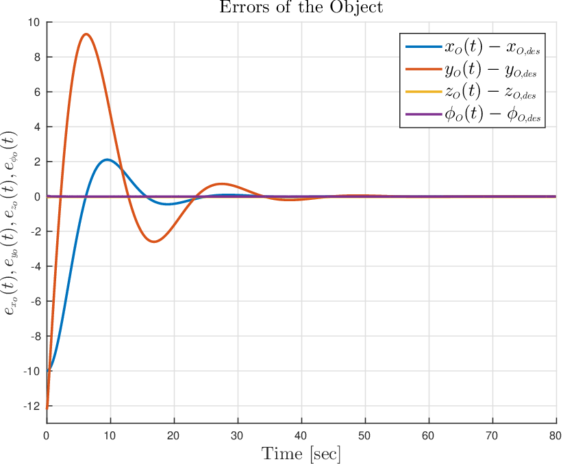
Refer to caption
Fig. 3: The errors of the object.
Refer to caption
Fig. 4: The velocities of the object.

V Simulation Results

To demonstrate the efficiency of the proposed control protocol, we consider two simulation scenarios.

Scenario 1: Consider N=2N=2 ground vehicles equipped with 22 DOF manipulators, rigidly grasping an object with n1=n2=4,n=n1+n2=8n_{1}=n_{2}=4,n=n_{1}+n_{2}=8. From (13) we have that x=[xO⊤,vO⊤,q⊤]⊤∈ℝ16,u∈ℝ8x=[x_{\scriptscriptstyle O}^{\top},v_{\scriptscriptstyle O}^{\top},q^{\top}]^{\top}\in\mathbb{R}^{16},u\in\mathbb{R}^{8}, with xO=[pO⊤,ϕO]⊤∈ℝ4x_{\scriptscriptstyle O}=[p_{\scriptscriptstyle O}^{\top},\phi_{\scriptscriptstyle O}]^{\top}\in\mathbb{R}^{4}, vO=[p˙O⊤,ωxO]⊤∈ℝ4v_{\scriptscriptstyle O}=[\dot{p}_{\scriptscriptstyle O}^{\top},\omega_{\scriptscriptstyle x_{O}}]^{\top}\in\mathbb{R}^{4}, pO=[xO,yO,zO]⊤∈ℝ3,q=[q1⊤,q2⊤]⊤∈ℝ8p_{\scriptscriptstyle O}=[x_{\scriptscriptstyle O},y_{\scriptscriptstyle O},z_{\scriptscriptstyle O}]^{\top}\in\mathbb{R}^{3},q=[q_{1}^{\top},q_{2}^{\top}]^{\top}\in\mathbb{R}^{8}, qi=[pBi⊤,αi⊤]⊤∈ℝ4q_{i}=[p_{\scriptscriptstyle B_{i}}^{\top},\alpha_{i}^{\top}]^{\top}\in\mathbb{R}^{4}, pBi=[xBi,yBi]⊤∈ℝ2p_{\scriptscriptstyle B_{i}}=[x_{\scriptscriptstyle B_{i}},y_{\scriptscriptstyle B_{i}}]^{\top}\in\mathbb{R}^{2}, αi=[αi1,αi2]⊤∈ℝ2,i∈{1,2}\alpha_{i}=[\alpha_{i_{1}},\alpha_{i_{2}}]^{\top}\in\mathbb{R}^{2},i\in\{1,2\}. The manipulators become singular when sin(αi1)=0},i∈{1,2}\sin(\alpha_{i_{1}})=0\},i\in\{1,2\}, thus the state constraints for the manipulators are set to:

ε<α11<π2−ε,\displaystyle\varepsilon<\alpha_{1_{1}}<\frac{\pi}{2}-\varepsilon, −π2+ε<α12<π2−ε,\displaystyle-\frac{\pi}{2}+\varepsilon<\alpha_{1_{2}}<\frac{\pi}{2}-\varepsilon,
−π2+ε<α21<−ε,\displaystyle-\frac{\pi}{2}+\varepsilon<\alpha_{2_{1}}<-\varepsilon, −π2+ε<α22<π2−ε.\displaystyle-\frac{\pi}{2}+\varepsilon<\alpha_{2_{2}}<\frac{\pi}{2}-\varepsilon.

We also consider the input constraints:

−10≤ui,j​(t)≤10,i∈{1,2},j∈{1,…,4}.-10\leq u_{i,j}(t)\leq 10,i\in\{1,2\},j\in\{1,\dots,4\}.

The initial conditions are set to:

xO​(0)\displaystyle x_{\scriptscriptstyle O}(0) =[0,−2.2071,0.9071,π2]⊤,vO​(0)=[0,0,0,0]⊤,\displaystyle=\left[0,-2.2071,0.9071,\frac{\pi}{2}\right]^{\top},v_{\scriptscriptstyle O}(0)=\left[0,0,0,0\right]^{\top},
q1​(0)\displaystyle q_{1}(0) =[0,0,π4,π4]⊤,q2​(0)=[0,−4.4142,−π4,−π4]⊤.\displaystyle=\left[0,0,\frac{\pi}{4},\frac{\pi}{4}\right]^{\top},q_{2}(0)=\left[0,-4.4142,-\frac{\pi}{4},-\frac{\pi}{4}\right]^{\top}.

The desired goal states are set to:

xO,des\displaystyle x_{\scriptscriptstyle O,\text{des}} =[10,10,0.9071,π2]⊤,vO,des=[0,0,0,0]⊤,\displaystyle=\left[10,10,0.9071,\frac{\pi}{2}\right]^{\top},v_{\scriptscriptstyle O,\text{des}}=\left[0,0,0,0\right]^{\top},
q1,des\displaystyle q_{1,\text{des}} =[10,12.2071,π4,π4]⊤,q2,des=[10,7.7929,−π4,−π4]⊤.\displaystyle=\left[10,12.2071,\frac{\pi}{4},\frac{\pi}{4}\right]^{\top},q_{2,\text{des}}=\left[10,7.7929,-\frac{\pi}{4},-\frac{\pi}{4}\right]^{\top}.

We set an obstacle between the initial and the desired pose of the object. the obstacle is spherical with center [5,5,1][5,5,1] and radius 22. The sampling time is h=0.1​sech=0.1\sec, the horizon is set to Tp=0.3​secT_{p}=0.3\sec, and the total simulation time is 80​sec80\sec; The matrices P,Q,RP,Q,R are set to:

P=Q=10​I16×16,R=2​I8×8.P=Q=10I_{16\times 16},R=2I_{8\times 8}.

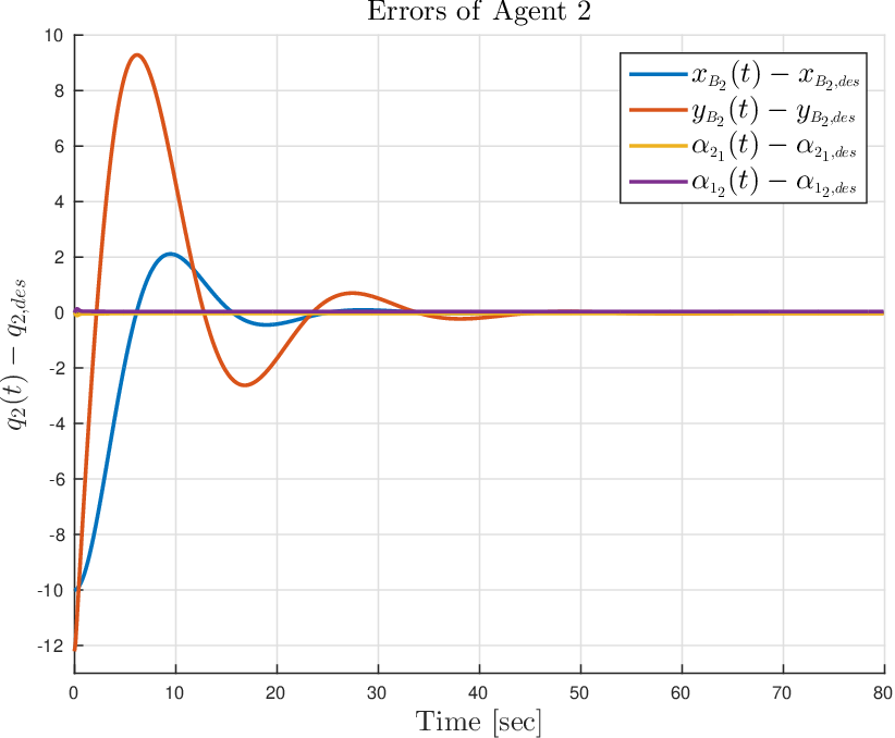
The simulation results are depicted in Fig. 3- Fig. 8, which shows that the states of the agents as well as the states of the object converge to the desired ones while guaranteeing that the obstacle is avoided and all state and input constraints are met.

Refer to caption
Fig. 5: The errors of vehicle 11 as well as the errors of the manipulator.
Refer to caption
Fig. 6: The errors of vehicle 22 as well as the errors of the manipulator.
Refer to caption
Fig. 7: The control inputs of the actuators of agent 11.
Refer to caption
Fig. 8: The control inputs of the actuators of agent 22.

Scenario 2: Consider N=3N=3 ground vehicles equipped with 22 DOF manipulators, rigidly grasping an object with n1=n2=n3=4,n=n1+n2+n3=12n_{1}=n_{2}=n_{3}=4,n=n_{1}+n_{2}+n_{3}=12. From (13) we have that x=[xO⊤,vO⊤,q⊤]⊤∈ℝ20x=[x_{\scriptscriptstyle O}^{\top},v_{\scriptscriptstyle O}^{\top},q^{\top}]^{\top}\in\mathbb{R}^{20}, u∈ℝ12u\in\mathbb{R}^{12}, with xO=[pO⊤,ϕO]⊤∈ℝ4x_{\scriptscriptstyle O}=[p_{\scriptscriptstyle O}^{\top},\phi_{\scriptscriptstyle O}]^{\top}\in\mathbb{R}^{4}, vO=[p˙O⊤,ωxO]⊤∈ℝ4v_{\scriptscriptstyle O}=[\dot{p}_{\scriptscriptstyle O}^{\top},\omega_{\scriptscriptstyle x_{O}}]^{\top}\in\mathbb{R}^{4}, pO=[xO,yO,zO]⊤∈ℝ3p_{\scriptscriptstyle O}=[x_{\scriptscriptstyle O},y_{\scriptscriptstyle O},z_{\scriptscriptstyle O}]^{\top}\in\mathbb{R}^{3}, q=[q1⊤,q2⊤,q3⊤]⊤∈ℝ12q=[q_{1}^{\top},q_{2}^{\top},q_{3}^{\top}]^{\top}\in\mathbb{R}^{12}, qi=[pBi⊤,αi⊤]⊤∈ℝ4q_{i}=[p_{\scriptscriptstyle B_{i}}^{\top},\alpha_{i}^{\top}]^{\top}\in\mathbb{R}^{4}, pBi=[xBi,yBi]⊤∈ℝ2p_{\scriptscriptstyle B_{i}}=[x_{\scriptscriptstyle B_{i}},y_{\scriptscriptstyle B_{i}}]^{\top}\in\mathbb{R}^{2}, αi=[αi1,αi2]⊤∈ℝ2,i∈{1,2}\alpha_{i}=[\alpha_{i_{1}},\alpha_{i_{2}}]^{\top}\in\mathbb{R}^{2},i\in\{1,2\}. The manipulators become singular when sin(αi1)=0},i∈{1,2,3}\sin(\alpha_{i_{1}})=0\},i\in\{1,2,3\}, thus the state constraints for the manipulators are set to:

ε<α11<π2−ε,\displaystyle\varepsilon<\alpha_{1_{1}}<\frac{\pi}{2}-\varepsilon, −π2+ε<α12<π2−ε,\displaystyle-\frac{\pi}{2}+\varepsilon<\alpha_{1_{2}}<\frac{\pi}{2}-\varepsilon,
−π2+ε<α21<−ε,\displaystyle-\frac{\pi}{2}+\varepsilon<\alpha_{2_{1}}<-\varepsilon, −π2+ε<α22<π2−ε.\displaystyle-\frac{\pi}{2}+\varepsilon<\alpha_{2_{2}}<\frac{\pi}{2}-\varepsilon.

We also consider the input constraints:

−10≤ui,j​(t)≤10,i∈{1,2},j∈{1,…,4}.-10\leq u_{i,j}(t)\leq 10,i\in\{1,2\},j\in\{1,\dots,4\}.

The initial conditions are set to:

xO​(0)\displaystyle x_{\scriptscriptstyle O}(0) =[0,−2.2071,0.9071,π2]⊤,vO​(0)=[0,0,0,0]⊤,\displaystyle=\left[0,-2.2071,0.9071,\frac{\pi}{2}\right]^{\top},v_{\scriptscriptstyle O}(0)=\left[0,0,0,0\right]^{\top},
q1​(0)\displaystyle q_{1}(0) =[0.5,0,π4,π4]⊤,q2​(0)=[0,−4.4142,−π4,−π4]⊤,\displaystyle=\left[0.5,0,\frac{\pi}{4},\frac{\pi}{4}\right]^{\top},q_{2}(0)=\left[0,-4.4142,-\frac{\pi}{4},-\frac{\pi}{4}\right]^{\top},
q3​(0)\displaystyle q_{3}(0) =[−0.5,0,π4,π4]⊤.\displaystyle=\left[-0.5,0,\frac{\pi}{4},\frac{\pi}{4}\right]^{\top}.

The desired goal states are set to:

xO,des\displaystyle x_{\scriptscriptstyle O,\text{des}} =[5,−2.2071,0.9071,π2]⊤,vO,des=[0,0,0,0]⊤,\displaystyle=\left[5,-2.2071,0.9071,\frac{\pi}{2}\right]^{\top},v_{\scriptscriptstyle O,\text{des}}=\left[0,0,0,0\right]^{\top},
q1,des\displaystyle q_{1,\text{des}} =[5.5,0,π4,π4]⊤,q2,des=[5,−4.4142,−π4,−π4]⊤,\displaystyle=\left[5.5,0,\frac{\pi}{4},\frac{\pi}{4}\right]^{\top},q_{2,\text{des}}=\left[5,-4.4142,-\frac{\pi}{4},-\frac{\pi}{4}\right]^{\top},
q3,des\displaystyle q_{3,\text{des}} =[4.5,0.0,π4,π4]⊤.\displaystyle=\left[4.5,0.0,\frac{\pi}{4},\frac{\pi}{4}\right]^{\top}.

The sampling time is h=0.1​sech=0.1\sec, the horizon is set to Tp=0.5​secT_{p}=0.5\sec, and the total simulation time is 100​sec100\sec; The matrices P,Q,RP,Q,R are set to:

P=Q=0.5​I20×20,R=0.5​I12×12.P=Q=0.5I_{20\times 20},R=0.5I_{12\times 12}.

The simulation results are depicted in Fig. 9- Fig. 16, which shows that the states of the agents as well as the states of the object converge to the desired ones while guaranteeing that all state and input constraints are met. The simulation scenarios were carried out by using the NMPC toolbox given in [25] and they took 23500​sec23500\sec, 45547​sec45547\sec for Scenario 11 and Scenario 22, respectively, in MATLAB Environment on a desktop with 88 cores, 3.603.60 GHz SPU and 1616GB of RAM.

VI Conclusions and Future Work

In this work we proposed a NMPC scheme for the cooperative transportation of an object rigidly grasped by NN robotic agents. The proposed control scheme deals with singularities of the agents, inter-agent collision avoidance as well as collision avoidance between the agents and the object with the workspace obstacles. We proved the feasibility and convergence analysis of the proposed methodology and simulation results verified the efficiency of the approach. Future efforts will be devoted towards including load sharing coefficients, internal force regulation, and complete decentralization of the proposed method. Finally, we will try to decrease the overall complexity and carry out real-time experiments.

Refer to caption
Fig. 9: The errors of the object.
Refer to caption
Fig. 10: The velocities of the object.
Refer to caption
Fig. 11: The errors of vehicle 11 as well as the errors of the manipulator.
Refer to caption
Fig. 12: The errors of vehicle 22 as well as the errors of the manipulator.
Refer to caption
Fig. 13: The errors of vehicle 33 as well as the errors of the manipulator.
Refer to caption
Fig. 14: The control inputs of the actuators of agent 11.
Refer to caption
Fig. 15: The control inputs of the actuators of agent 33.
Refer to caption
Fig. 16: The control inputs of the actuators of agent 33.

Appendix A Proof of Lemma 2

By invoking the fact that:

λmin​(P)​‖y‖2≤y⊤​P​y≤λmax​(P)​‖y‖2,∀y∈ℝn,P∈ℝn×n,P=P⊤>0,\displaystyle\lambda_{\min}(P)\|y\|^{2}\leq y^{\top}Py\leq\lambda_{\max}(P)\|y\|^{2},\forall y\in\mathbb{R}^{n},P\in\mathbb{R}^{n\times n},P=P^{\top}>0, (26)

we have:

e⊤​Q​e+u⊤​R​u\displaystyle e^{\top}Qe+u^{\top}Ru ≤λmax​(Q)​‖e‖2+λmax​(R)​‖u‖2=max⁡{λmax​(Q),λmax​(R)}​‖z‖2,\displaystyle\leq\lambda_{\max}(Q)\|e\|^{2}+\lambda_{\max}(R)\|u\|^{2}=\max\{\lambda_{\max}(Q),\lambda_{\max}(R)\}\|z\|^{2},

and:

e⊤​Q​e+u⊤​R​u\displaystyle e^{\top}Qe+u^{\top}Ru ≥λmin​(Q)​‖e‖2+λmin​(R)​‖u‖2\displaystyle\geq\lambda_{\min}(Q)\|e\|^{2}+\lambda_{\min}(R)\|u\|^{2}
=min⁡{λmin​(Q),λmin​(R)}​‖z‖2,\displaystyle=\min\{\lambda_{\min}(Q),\lambda_{\min}(R)\}\|z\|^{2},

where z=[e⊤,u⊤]⊤z=\left[e^{\top},u^{\top}\right]^{\top}. Thus, we get:

min⁡{λmin​(Q),λmin​(R)}​‖z‖2\displaystyle\min\{\lambda_{\min}(Q),\lambda_{\min}(R)\}\|z\|^{2} ≤e⊤​Q​e+u⊤​R​u≤max⁡{λmax​(Q),λmax​(R)}​‖z‖2.\displaystyle\leq e^{\top}Qe+u^{\top}Ru\leq\max\{\lambda_{\max}(Q),\lambda_{\max}(R)\}\|z\|^{2}.

By defining the 𝒦∞\mathcal{K}_{\infty} functions α1\alpha_{1}, α2:ℝ≥0→ℝ≥0\alpha_{2}:\mathbb{R}_{\geq 0}\to\mathbb{R}_{\geq 0}:

α1​(y)≜m​‖y‖2,α2​(y)≜max⁡{λmax​(Q),λmax​(R)}​‖y‖2,\displaystyle\alpha_{1}(y)\triangleq m\|y\|^{2},\alpha_{2}(y)\triangleq\max\{\lambda_{\max}(Q),\lambda_{\max}(R)\}\|y\|^{2},

and the parameter m∈ℝ>0m\in\mathbb{R}_{>0} by:

m≜min⁡{λmin​(Q),λmin​(R)},\displaystyle m\triangleq\min\{\lambda_{\min}(Q),\lambda_{\min}(R)\}, (27)

we get:

α1​(‖z‖)≤F⁡(e,u)≤α2​(‖z‖),\displaystyle\alpha_{1}\big(\|z\|\big)\leq F\big(e,u\big)\leq\alpha_{2}\big(\|z\|\big), (28)

which leads to the conclusion of the proof. ∎

Appendix B Proof of Lemma 2

Proof.

For every e⁡(t)∈ℰfe(t)\in\mathcal{E}_{f}, the following holds:

|V⁡(e1)−V⁡(e2)|\displaystyle|V(e_{1})-V(e_{2})| =|e1⊤​P​e1−e2⊤​P​e2|\displaystyle=|e_{1}^{\top}Pe_{1}-e_{2}^{\top}Pe_{2}|
=|e1⊤​P​e1+e1⊤​P​e2−e1⊤​P​e2−e2⊤​P​e2|\displaystyle=|e_{1}^{\top}Pe_{1}+e_{1}^{\top}Pe_{2}-e_{1}^{\top}Pe_{2}-e_{2}^{\top}Pe_{2}|
=|e1⊤​P​(e1−e2)−e2⊤​P​(e1−e2)|\displaystyle=|e_{1}^{\top}P(e_{1}-e_{2})-e_{2}^{\top}P(e_{1}-e_{2})|
≤|e1⊤​P​(e1−e2)|+|e2⊤​P​(e1−e2)|.\displaystyle\leq|e_{1}^{\top}P(e_{1}-e_{2})|+|e_{2}^{\top}P(e_{1}-e_{2})|. (29)

By employing the property that:

|x⊤​A​y|≤σmax​(A)​‖x‖​‖y‖,∀x,y∈ℝn,A∈ℝn×n,|x^{\top}Ay|\leq\sigma_{\max}(A)\|x\|\|y\|,\forall\ x,y\in\mathbb{R}^{n},A\in\mathbb{R}^{n\times n},

(29) is written as:

|V⁡(e1)−V⁡(e2)|\displaystyle|V(e_{1})-V(e_{2})| ≤σmax​(P)​‖e1‖​‖e1−e2‖+σmax​(P)​‖e2‖​‖e1−e2‖\displaystyle\leq\sigma_{\max}(P)\|e_{1}\|\|e_{1}-e_{2}\|+\sigma_{\max}(P)\|e_{2}\|\|e_{1}-e_{2}\|
=σmax​(P)​(‖e1‖+‖e2‖)​‖e1−e2‖\displaystyle=\sigma_{\max}(P)(\|e_{1}\|+\|e_{2}\|)\|e_{1}-e_{2}\|
≤σmax​(P)​(ε0+ε0)​‖e1−e2‖\displaystyle\leq\sigma_{\max}(P)(\varepsilon_{0}+\varepsilon_{0})\|e_{1}-e_{2}\|
=[2​ε0​σmax​(P)]​‖e1−e2‖.\displaystyle=\left[2\varepsilon_{0}\sigma_{\max}(P)\right]\|e_{1}-e_{2}\|.

which completes the proof. ∎

Appendix C Feasibility Analysis

Consider any sampling time instant tit_{i} for which a solution exists. In between tit_{i} and ti+1t_{i+1}, the optimal control input u^⋆​(s,e⁡(ti)),s∈[ti,ti+1)\hat{u}^{\star}(s;e(t_{i})),s\in[t_{i},t_{i+1}) is implemented. According to (25), it holds that:

e⁡(ti+1)=e^​(ti+1,u^⋆​(⋅,e⁡(ti)),e⁡(ti)).e(t_{i+1})=\hat{e}(t_{i+1};\hat{u}^{\star}(\cdot;e(t_{i})),e(t_{i})).

The remaining piece of the optimal control input u^⋆​(s,e⁡(ti)),s∈[ti+1,ti+Tp]\hat{u}^{\star}(s;e(t_{i})),s\in[t_{i+1},t_{i}+T_{p}] satisfies the state and input constraints E,UE,U, respectively. Furthermore,

e^​(ti+Tp,u^⋆​(⋅,e⁡(ti)),e⁡(ti))∈ℰf,\hat{e}(t_{i}+T_{p};\hat{u}^{\star}(\cdot;e(t_{i})),e(t_{i}))\in\mathcal{E}_{f},

and we know from Assumption 2b of Theorem 1 that for all e⁡(t)∈ℰfe(t)\in\mathcal{E}_{f}, there exists at least one control input uf​(⋅)u_{f}(\cdot) that renders the set ℰf\mathcal{E}_{f} invariant over hh. Picking any such input, a feasible control input u¯​(⋅,e​(ti+1))\bar{u}(\cdot;e(t_{i+1})), at time instant ti+1t_{i+1}, may be the following:

u¯​(s,e⁡(ti+1))={u^⋆(s;e(ti)),s∈[ti+1,ti+Tp],uf​(e^​(ti+Tp,u⋆​(⋅),e⁡(ti))),s∈[ti+Tp,ti+1+Tp].\displaystyle\bar{u}(s;e(t_{i+1}))=\begin{cases}\hat{u}^{\star}(s;e(t_{i})),\qquad&s\in[t_{i+1},t_{i}+T_{p}],\\ u_{f}(\hat{e}(t_{i}+T_{p};u^{\star}(\cdot),e(t_{i}))),&s\in[t_{i}+T_{p},t_{i+1}+T_{p}].\end{cases} (30)

Thus, from feasibility of u^⋆​(s,e⁡(ti))\hat{u}^{\star}(s,e(t_{i})) and the fact that uf​(e​(t))∈Uu_{f}(e(t))\in U, for all e⁡(t)∈ℰfe(t)\in\mathcal{E}_{f}, it follows that:

u¯​(s,e⁡(ti+1))∈U,∀s∈[ti+1,ti+Tp].\bar{u}(s;e(t_{i+1}))\in U,\forall\ s\in[t_{i+1},t_{i}+T_{p}].

Hence, the feasibility at time tit_{i} implies feasibility at time ti+1t_{i+1}. Therefore, if the OCP (21a) - (21d) is feasible at time t=0t=0, it remains feasible for every t≥0t\geq 0.

Appendix D Convergence Analysis

The second part involves proving convergence of the state ee in the terminal set ℰf\mathcal{E}_{f}. In order to prove this, it must be shown that a proper value function is decreasing along the solution trajectories starting at a sampling time tit_{i}. Consider the optimal value function J⋆​(e⁡(ti))J^{\star}(e(t_{i})), as is given in (24). Consider also the cost of the feasible control input, indicated by:

J¯​(e⁡(ti+1))≜J¯​(e⁡(ti+1),u¯​(⋅,e⁡(ti+1))),\bar{J}(e(t_{i+1}))\triangleq\bar{J}(e(t_{i+1}),\bar{u}(\cdot;e(t_{i+1}))), (31)

where ti+1=ti+ht_{i+1}=t_{i}+h, as is given in (20). Define:

u1​(s)\displaystyle u_{1}(s) =u¯​(s,e​(ti+1)),\displaystyle=\bar{u}(s;e(t_{i+1})), (32)
e1​(s)\displaystyle e_{1}(s) =e¯​(s,u1​(s),e⁡(ti+1)),s>ti+1.\displaystyle=\bar{e}(s;u_{1}(s),e(t_{i+1})),s>t_{i+1}.

e1​(s)e_{1}(s) stands for the predicted state ee at time ss, based on the measurement of the state ee at time ti+1t_{i+1}, while using the feasible control input u¯​(s,e​(ti+1))\bar{u}(s;e(t_{i+1})). Let us also define th the following terms:

u2​(s)\displaystyle u_{2}(s) =u^⋆​(s,e⁡(ti)),\displaystyle=\hat{u}^{\star}(s;e(t_{i})), (33)
e2​(s)\displaystyle e_{2}(s) =e^​(s,u2​(s),e⁡(ti)),s>ti+1.\displaystyle=\hat{e}(s;u_{2}(s),e(t_{i})),s>t_{i+1}.

(32), (33) form convenient notations for the readability of the proof hereafter.

By employing (21a), (24) and (31), the difference between the optimal and feasible cost is given by:

J¯​(e⁡(ti+1))−J⋆​(e⁡(ti))=V⁡(e1​(ti+1+Tp))+∫ti+1ti+1+Tp[F⁡(e1​(s),u1​(s))]​𝑑s\displaystyle\bar{J}(e(t_{i+1}))-J^{\star}(e(t_{i}))=V(e_{1}(t_{i+1}+T_{p}))+\int_{t_{i+1}}^{t_{i+1}+T_{p}}\Big[F(e_{1}(s),u_{1}(s))\Big]ds
−V⁡(e2​(ti+Tp))−∫titi+Tp[F⁡(e2​(s),u2​(s))]​𝑑s\displaystyle\hskip 22.76219pt-V(e_{2}(t_{i}+T_{p}))-\int_{t_{i}}^{t_{i}+T_{p}}\Big[F(e_{2}(s),u_{2}(s))\Big]ds
=V⁡(e1​(ti+1+Tp))+∫ti+1ti+Tp[F⁡(e1​(s),u1​(s))]​𝑑s\displaystyle=V(e_{1}(t_{i+1}+T_{p}))+\int_{t_{i+1}}^{t_{i}+T_{p}}\Big[F(e_{1}(s),u_{1}(s))\Big]ds
+∫ti+Tpti+1+Tp[F(e1(s),u1(s))]ds−V(e2(ti+Tp))\displaystyle+\int_{t_{i}+T_{p}}^{t_{i+1}+T_{p}}\Big[F(e_{1}(s),u_{1}(s))\Big]ds-V(e_{2}(t_{i}+T_{p}))
−∫titi+1[F(e2(s),u2(s))]ds−∫ti+1ti+Tp[F(e2(s),u2(s))]ds.\displaystyle\hskip 42.67912pt-\int_{t_{i}}^{t_{i+1}}\Big[F(e_{2}(s),u_{2}(s))\Big]ds-\int_{t_{i+1}}^{t_{i}+T_{p}}\Big[F(e_{2}(s),u_{2}(s))\Big]ds. (34)

Note that, from (30), the following holds:

u¯​(s,e⁡(ti+1))=u^⋆​(s,e⁡(ti)),∀s∈[ti+1,ti+Tp].\bar{u}(s;e(t_{i+1}))=\hat{u}^{\star}(s;e(t_{i})),\forall\ s\in[t_{i+1},t_{i}+T_{p}]. (35)

By combining (32), (33) and (35), it yields that:

u1​(s)=u2​(s)=u¯​(s),∀s∈[ti+1,ti+Tp],u_{1}(s)=u_{2}(s)=\bar{u}(s),\forall\ s\in[t_{i+1},t_{i}+T_{p}], (36)

which implies that:

e1​(s)=e2​(s),∀s∈[ti+1,ti+Tp].e_{1}(s)=e_{2}(s),\forall\ s\in[t_{i+1},t_{i}+T_{p}]. (37)

The combination of (36) and (37) implies that:

F⁡(e1​(s),u1​(s))=F⁡(e1​(s),u1​(s)),∀s∈[ti+1,ti+Tp].F(e_{1}(s),u_{1}(s))=F(e_{1}(s),u_{1}(s)),\forall\ s\in[t_{i+1},t_{i}+T_{p}].

which implies that:

∫ti+1ti+Tp[F⁡(e1​(s),u1​(s))]​𝑑s=∫ti+1ti+Tp[F⁡(e2​(s),u2​(s))]​𝑑s.\displaystyle\int_{t_{i+1}}^{t_{i}+T_{p}}\Big[F(e_{1}(s),u_{1}(s))\Big]ds=\int_{t_{i+1}}^{t_{i}+T_{p}}\Big[F(e_{2}(s),u_{2}(s))\Big]ds. (38)

By employing (38), (34) becomes:

J¯​(e⁡(ti+1))−J⋆​(e⁡(ti))=\displaystyle\bar{J}(e(t_{i+1}))-J^{\star}(e(t_{i}))=\ V⁡(e1​(ti+1+Tp))+∫ti+Tpti+1+Tp[F⁡(e1​(s),u1​(s))]​𝑑s\displaystyle V(e_{1}(t_{i+1}+T_{p}))+\int_{t_{i}+T_{p}}^{t_{i+1}+T_{p}}\Big[F(e_{1}(s),u_{1}(s))\Big]ds
−V⁡(e2​(ti+Tp))−∫titi+1[F⁡(e2​(s),u2​(s))]​𝑑s.\displaystyle-V(e_{2}(t_{i}+T_{p}))-\int_{t_{i}}^{t_{i+1}}\Big[F(e_{2}(s),u_{2}(s))\Big]ds. (39)

Due to the fact that ti+1+Tp−(ti+Tp)=ti+1−ti=ht_{i+1}+T_{p}-(t_{i}+T_{p})=t_{i+1}-t_{i}=h, and the Assumption 2b of Theorem 1 holds for one sampling period hh, by integrating this inequality from ti+Tpt_{i}+T_{p} to ti+1+Tpt_{i+1}+T_{p} and we get the following:

∫ti+Tpti+1+Tp[∂V∂e​fe​(e1​(s),u1​(s))+F⁡(e1​(s),u1​(s))]​𝑑s≤0\displaystyle\hskip-8.53581pt\int_{t_{i}+T_{p}}^{t_{i+1}+T_{p}}\Big[\frac{\partial V}{\partial{e}}f_{e}(e_{1}(s),u_{1}(s))+F(e_{1}(s),u_{1}(s))\Big]ds\leq 0
⇔\displaystyle\Leftrightarrow ∫ti+Tpti+1+Tp[V˙​(e1​(s))]​𝑑s+∫ti+Tpti+1+Tp[F⁡(e1​(s),u1​(s))]​𝑑s≤0\displaystyle\int_{t_{i}+T_{p}}^{t_{i+1}+T_{p}}\Big[\dot{V}(e_{1}(s))\Big]ds+\int_{t_{i}+T_{p}}^{t_{i+1}+T_{p}}\Big[F(e_{1}(s),u_{1}(s))\Big]ds\leq 0
⇔\displaystyle\Leftrightarrow V⁡(e1​(ti+1+Tp))−V⁡(e1​(ti+Tp))+∫ti+Tpti+1+Tp[F⁡(e1​(s),u1​(s))]​𝑑s≤0\displaystyle V(e_{1}(t_{i+1}+T_{p}))-V(e_{1}(t_{i}+T_{p}))+\int_{t_{i}+T_{p}}^{t_{i+1}+T_{p}}\Big[F(e_{1}(s),u_{1}(s))\Big]ds\leq 0
⇔\displaystyle\Leftrightarrow V⁡(e1​(ti+1+Tp))−V⁡(e1​(ti+Tp))+∫ti+Tpti+1+Tp[F⁡(e1​(s),u1​(s))]​𝑑s≤\displaystyle V(e_{1}(t_{i+1}+T_{p}))-V(e_{1}(t_{i}+T_{p}))+\int_{t_{i}+T_{p}}^{t_{i+1}+T_{p}}\Big[F(e_{1}(s),u_{1}(s))\Big]ds\leq
V⁡(e2​(ti+Tp))−V⁡(e2​(ti+Tp))\displaystyle\hskip 71.13188ptV(e_{2}(t_{i}+T_{p}))-V(e_{2}(t_{i}+T_{p}))
⇔\displaystyle\Leftrightarrow V⁡(e1​(ti+1+Tp))+∫ti+Tpti+1+Tp[F⁡(e1​(s),u1​(s))]​𝑑s−V⁡(e2​(ti+Tp))≤\displaystyle V(e_{1}(t_{i+1}+T_{p}))+\int_{t_{i}+T_{p}}^{t_{i+1}+T_{p}}\Big[F(e_{1}(s),u_{1}(s))\Big]ds-V(e_{2}(t_{i}+T_{p}))\leq
V⁡(e1​(ti+Tp))−V⁡(e2​(ti+Tp)).\displaystyle\hskip 62.59605ptV(e_{1}(t_{i}+T_{p}))-V(e_{2}(t_{i}+T_{p})).

By employing the property y≤|y|,∀y∈ℝy\leq|y|,\forall y\in\mathbb{R}, we get:

V⁡(e1​(ti+1+Tp))+∫ti+Tpti+1+Tp[F⁡(e1​(s),u1​(s))]​𝑑s−V⁡(e2​(ti+Tp))≤\displaystyle V(e_{1}(t_{i+1}+T_{p}))+\int_{t_{i}+T_{p}}^{t_{i+1}+T_{p}}\Big[F(e_{1}(s),u_{1}(s))\Big]ds-V(e_{2}(t_{i}+T_{p}))\leq
|V⁡(e1​(ti+Tp))−V⁡(e2​(ti+Tp))|.\displaystyle\hskip 42.67912pt\left|V(e_{1}(t_{i}+T_{p}))-V(e_{2}(t_{i}+T_{p}))\right|. (40)

By employing Lemma 2, we have that:

|V⁡(e1​(ti+Tp))−V⁡(e2​(ti+Tp))|≤LV​‖e1​(ti+Tp)−e2​(ti+Tp)‖.\displaystyle\left|V(e_{1}(t_{i}+T_{p}))-V(e_{2}(t_{i}+T_{p}))\right|\leq L_{V}\|e_{1}(t_{i}+T_{p})-e_{2}(t_{i}+T_{p})\|. (41)

By combining (40) and (41) we get:

V⁡(e1​(ti+1+Tp))+∫ti+Tpti+1+Tp[F⁡(e1​(s),u1​(s))]​𝑑s−V⁡(e2​(ti+Tp))≤\displaystyle V(e_{1}(t_{i+1}+T_{p}))+\int_{t_{i}+T_{p}}^{t_{i+1}+T_{p}}\Big[F(e_{1}(s),u_{1}(s))\Big]ds-V(e_{2}(t_{i}+T_{p}))\leq
LV​‖e1​(ti+Tp)−e2​(ti+Tp)‖\displaystyle\hskip 71.13188ptL_{V}\|e_{1}(t_{i}+T_{p})-e_{2}(t_{i}+T_{p})\| (42)

For s=ti+Tps=t_{i}+T_{p}, (37) gives:

e1​(ti+Tp)=e2​(ti+Tp).e_{1}(t_{i}+T_{p})=e_{2}(t_{i}+T_{p}). (43)

By combining (43) and (42) we have:

V⁡(e1​(ti+1+Tp))+\displaystyle\hskip-6.54413ptV(e_{1}(t_{i+1}+T_{p}))+
∫ti+Tpti+1+Tp[F⁡(e1​(s),u1​(s))]​𝑑s−V⁡(e2​(ti+Tp))≤0.\displaystyle\hskip-6.54413pt\int_{t_{i}+T_{p}}^{t_{i+1}+T_{p}}\Big[F(e_{1}(s),u_{1}(s))\Big]ds-V(e_{2}(t_{i}+T_{p}))\leq 0. (44)

By combining (39) with (44), the following holds:

J¯(e(ti+1))−J⋆(e(ti))≤−∫titi+1[F(e2(s),u2(s))]ds.\displaystyle\bar{J}(e(t_{i+1}))-J^{\star}(e(t_{i}))\leq-\int_{t_{i}}^{t_{i+1}}\Big[F(e_{2}(s),u_{2}(s))\Big]ds. (45)

By substituting e=e2​(s),u=u2​(s)e=e_{2}(s),u=u_{2}(s) in (28) we get:

F⁡(e2​(s),u2​(s))≥m​‖z2​(s)‖2,F(e_{2}(s),u_{2}(s))\geq m\|z_{2}(s)\|^{2},

where z2≜[e2,u2]⊤z_{2}\triangleq[e_{2},u_{2}]^{\top}. The latter is equivalent to:

∫titi+1[F⁡(e2​(s),u2​(s))]​𝑑s≥m​∫titi+1‖z2​(s)‖2​𝑑s\displaystyle\int_{t_{i}}^{t_{i+1}}\Big[F(e_{2}(s),u_{2}(s))\Big]ds\geq m\int_{t_{i}}^{t_{i+1}}\|z_{2}(s)\|^{2}ds
⇔\displaystyle\Leftrightarrow −∫titi+1[F(e2(s),u2(s))]ds≤−m∫titi+1∥z2(s)∥2ds.\displaystyle-\int_{t_{i}}^{t_{i+1}}\Big[F(e_{2}(s),u_{2}(s))\Big]ds\leq-m\int_{t_{i}}^{t_{i+1}}\|z_{2}(s)\|^{2}ds. (46)

By combining (45) and (46) we finally get:

J¯(e(ti+1))−J⋆(e(ti))≤−m∫titi+1∥z2(s)∥2ds.\displaystyle\bar{J}(e(t_{i+1}))-J^{\star}(e(t_{i}))\leq-m\int_{t_{i}}^{t_{i+1}}\|z_{2}(s)\|^{2}ds. (47)

It is clear that the optimal solution at time ti+1t_{i+1} i.e., J⋆​(e⁡(ti+1))J^{\star}(e(t_{i+1})) will not be worse than the feasible one at the same time i.e. J¯​(e​(ti+1))\bar{J}(e(t_{i+1})). Therefore, (47) implies:

J⋆(e(ti+1))−J⋆(e(ti))≤−m∫titi+1∥z2(s)∥2s≤0,J^{\star}(e(t_{i+1}))-J^{\star}(e(t_{i}))\leq-m\int_{t_{i}}^{t_{i+1}}\|z_{2}(s)\|^{2}s\leq 0, (48)

or, by using the fact that ∫t0ti‖z2​(s)‖2​𝑑s\displaystyle\int_{t_{0}}^{t_{i}}\|z_{2}(s)\|^{2}ds =∑j=0i−1∫tjtj+1‖z2​(s)‖2​𝑑s=\displaystyle\sum_{j=0}^{i-1}\int_{t_{j}}^{t_{j+1}}\|z_{2}(s)\|^{2}ds, equivalently, we obtain:

J⋆(e(ti+1))−J⋆(e(ti))≤−m∫t0ti+1∥z2(s)∥2ds+m∑j=0i−1∫tjtj+1∥z2(s)∥2ds.\displaystyle J^{\star}(e(t_{i+1}))-J^{\star}(e(t_{i}))\leq-m\int_{t_{0}}^{t_{i+1}}\|z_{2}(s)\|^{2}ds+m\sum_{j=0}^{i-1}\int_{t_{j}}^{t_{j+1}}\|z_{2}(s)\|^{2}ds. (49)

By using induction and the fact that ti=h⋅i,ti+1=h⋅(i+1),∀i≥0t_{i}=h\cdot i,t_{i+1}=h\cdot(i+1),\forall i\geq 0, from (20), (49) is written as:

J⋆(e(ti))−J⋆(e(t0))≤−m∫t0ti∥z2(s)∥2ds.J^{\star}(e(t_{i}))-J^{\star}(e(t_{0}))\leq-m\int_{t_{0}}^{t_{i}}\|z_{2}(s)\|^{2}ds. (50)

Since t0=0t_{0}=0 we obtain:

J⋆​(e⁡(ti))≤J⋆​(e⁡(0))−m​∫0ti‖z2​(s)‖2​𝑑s.J^{\star}(e(t_{i}))\leq J^{\star}(e(0))-m\int_{0}^{t_{i}}\|z_{2}(s)\|^{2}ds. (51)

which implies that:

J⋆​(e⁡(ti))≤J⋆​(e⁡(0)).J^{\star}(e(t_{i}))\leq J^{\star}(e(0)). (52)

By combining (48), (52), we obtain:

J⋆​(e⁡(ti+1))≤J⋆​(e⁡(ti))≤J⋆​(e⁡(0)),∀ti=i⋅h,i≥0.J^{\star}(e(t_{i+1}))\leq J^{\star}(e(t_{i}))\leq J^{\star}(e(0)),\forall\ t_{i}=i\cdot h,i\geq 0. (53)

Therefore, the value function J⋆​(e⁡(ti))J^{\star}(e(t_{i})) has proven to be non-increasing for all the sampling times. Let us define the function:

V⁡(e⁡(t))=J⋆​(e⁡(s))≤J⋆​(e⁡(0)),t∈ℝ≥0,V(e(t))=J^{\star}(e(s))\leq J^{\star}(e(0)),t\in\mathbb{R}_{\geq 0}, (54)

where s=max⁡{ti:ti≤t}s=\max\{t_{i}:t_{i}\leq t\}. Since J⋆​(e​(0))J^{\star}(e(0)) is bounded, (54) implies that V⁡(e⁡(t))V(e(t)) is bounded. Since the signals e⁡(t),u⁡(t)e(t),u(t) are bounded (e⁡(t)∈E,u⁡(t)∈Ue(t)\in E,u(t)\in U), according to (16), it holds that e˙​(t)\dot{e}(t) is also bounded. From (51) we have that:

V⁡(e⁡(t))=J⋆​(e⁡(s))≤J⋆​(e⁡(0))−m​∫0s‖z2​(s)‖2​𝑑s.V(e(t))=J^{\star}(e(s))\leq J^{\star}(e(0))-m\int_{0}^{s}\|z_{2}(s)\|^{2}ds.

which due to the fact that s≤ts\leq t, is equivalent to:

V⁡(e⁡(t))≤J⋆​(e⁡(0))−m​∫0t‖z2​(s)‖2​𝑑s,t∈ℝ≥0.V(e(t))\leq J^{\star}(e(0))-m\int_{0}^{t}\|z_{2}(s)\|^{2}ds,t\in\mathbb{R}_{\geq 0}. (55)

From (55), we get:

∫0t‖z2​(s)‖2​𝑑s≤1m​[J⋆​(e⁡(0))−V⁡(e⁡(t))],t∈ℝ≥0.\int_{0}^{t}\|z_{2}(s)\|^{2}ds\leq\frac{1}{m}\left[J^{\star}(e(0))-V(e(t))\right],t\in\mathbb{R}_{\geq 0}. (56)

Since J⋆​(e⁡(0)),V⁡(e⁡(t))J^{\star}(e(0)),V(e(t)) has been proven to be bounded, the term ∫0t‖z2​(s)‖2​𝑑s\displaystyle\int_{0}^{t}\|z_{2}(s)\|^{2}ds is also bounded. Therefore, by employing Lemma 1, we have that ‖z2​(t)‖→0\|z_{2}(t)\|\to 0, as t→∞t\to\infty. The latter implies that:

limt→∞‖e⁡(t)‖=0⇒e⁡(t)∈ℰf,as​t→∞,\lim_{t\to\infty}\|e(t)\|=0\Rightarrow e(t)\in\mathcal{E}_{f},\ \text{as}\ t\to\infty,

and leads to the conclusion of the proof.

References

  • [1] S. A. Schneider and R. H. Cannon, “Object impedance control for cooperative manipulation: Theory and experimental results,” IEEE Transactions on Robotics and Automation, vol. 8, no. 3, pp. 383–394, 1992.
  • [2] Y.-H. Liu, S. Arimoto, and T. Ogasawara, “Decentralized cooperation control: non-communication object handling,” Proceedings of the IEEE Conference on Robotics and Automation (ICRA), vol. 3, pp. 2414–2419, 1996.
  • [3] Y.-H. Liu and S. Arimoto, “Decentralized adaptive and nonadaptive position/force controllers for redundant manipulators in cooperations,” The International Journal of Robotics Research, vol. 17, no. 3, pp. 232–247, 1998.
  • [4] M. Zribi and S. Ahmad, “Adaptive control for multiple cooperative robot arms,” Proceedings of the IEEE International Conference on Decision and Control (CDC), pp. 1392–1398, 1992.
  • [5] O. Khatib, K. Yokoi, K. Chang, D. Ruspini, R. Holmberg, and A. Casal, “Decentralized cooperation between multiple manipulators,” IEEE International Workshop on Robot and Human Communication, pp. 183–188, 1996.
  • [6] F. Caccavale, P. Chiacchio, and S. Chiaverini, “Task-space regulation of cooperative manipulators,” Automatica, vol. 36, no. 6, pp. 879–887, 2000.
  • [7] J. Gudiño-Lau, M. A. Arteaga, L. A. Munoz, and V. Parra-Vega, “On the control of cooperative robots without velocity measurements,” IEEE Transactions on Control Systems Technology, vol. 12, no. 4, pp. 600–608, 2004.
  • [8] F. Caccavale, P. Chiacchio, A. Marino, and L. Villani, “Six-dof impedance control of dual-arm cooperative manipulators,” IEEE/ASME Transactions On Mechatronics, vol. 13, no. 5, pp. 576–586, 2008.
  • [9] D. Heck, D. Kostić, A. Denasi, and H. Nijmeijer, “Internal and external force-based impedance control for cooperative manipulation,” Proceedings of the IEEE European Control Conference (ECC), pp. 2299–2304, 2013.
  • [10] S. Erhart and S. Hirche, “Adaptive force/velocity control for multi-robot cooperative manipulation under uncertain kinematic parameters,” Proceedings of the IEEE/RSJ International Conference on Intelligent Robots and Systems (IROS), pp. 307–314, 2013.
  • [11] S. Erhart, D. Sieber, and S. Hirche, “An impedance-based control architecture for multi-robot cooperative dual-arm mobile manipulation,” Proceedings of the IEEE/RSJ International Conference on Intelligent Robots and Systems (IROS), pp. 315–322, 2013.
  • [12] J. Szewczyk, F. Plumet, and P. Bidaud, “Planning and controlling cooperating robots through distributed impedance,” Journal of Robotic Systems, vol. 19, no. 6, pp. 283–297, 2002.
  • [13] A. Tsiamis, C. K. Verginis, C. P. Bechlioulis, and K. J. Kyriakopoulos, “Cooperative manipulation exploiting only implicit communication,” Proceedings of the IEEE/RSJ International Conference on Intelligent Robots and Systems (IROS), pp. 864–869, 2015.
  • [14] F. Ficuciello, A. Romano, L. Villani, and B. Siciliano, “Cartesian impedance control of redundant manipulators for human-robot co-manipulation,” Proceedings of the IEEE/RSJ International Conference on Intelligent Robots and Systems (IROS), pp. 2120–2125, 2014.
  • [15] A. Ponce-Hinestroza, J. Castro-Castro, H. Guerrero-Reyes, V. Parra-Vega, and E. Olguỳn-Dỳaz, “Cooperative redundant omnidirectional mobile manipulators: Model-free decentralized integral sliding modes and passive velocity fields,” Proceedings of the IEEE International Conference on Robotics and Automation (ICRA), pp. 2375–2380, 2016.
  • [16] W. Gueaieb, F. Karray, and S. Al-Sharhan, “A robust hybrid intelligent position/force control scheme for cooperative manipulators,” IEEE/ASME Transactions on Mechatronics, vol. 12, no. 2, pp. 109–125, 2007.
  • [17] M. Ciocarlie, F. M. Hicks, R. Holmberg, J. Hawke, M. Schlicht, J. Gee, S. Stanford, and R. Bahadur, “The velo gripper: A versatile single-actuator design for enveloping, parallel and fingertip grasps,” The International Journal of Robotics Research, 2014.
  • [18] D. E. Koditschek and E. Rimon, “Robot navigation functions on manifolds with boundary,” Advances in applied mathematics, vol. 11, no. 4, pp. 412–442, 1990.
  • [19] B.Siciliano, L. Sciavicco, and L. Villani, “Robotics: Modelling, Planning and Control”. Advanced Textbooks in Control and Signal Processing, Springer, 2009.
  • [20] K. S. de Oliveira and M. Morari, “Contractive Model Predictive Control for Constrained Nonlinear Systems,” IEEE Transactions on Automatic Control, vol. 45, no. 6, pp. 1053–1071, 2000.
  • [21] R. Findeisen, L. Imsland, F. Allgower, and B. A. Foss, “State and Output Feedback Nonlinear Model Predictive Control: An Overview,” European Journal of Control, vol. 9, no. 2-3, pp. 190–206, 2003.
  • [22] H. Chen and F. Allgöwer, “A Quasi-Infinite Horizon Nonlinear Model Predictive Control Scheme with Guaranteed Stability,” Automatica, vol. 34, no. 10, pp. 1205–1217, 1998.
  • [23] R. Findeisen, L. Imsland, F. Allgöwer, and B. Foss, “Towards a Sampled-Data Theory for Nonlinear Model Predictive Control,” New Trends in Nonlinear Dynamics and Control and their Applications, pp. 295–311, 2003.
  • [24] F. Fontes, “A General Framework to Design Stabilizing Nonlinear Model Predictive Controllers,” Systems and Control Letters, vol. 42, no. 2, pp. 127–143, 2001.
  • [25] L. Grüne and J. Pannek, Nonlinear Model Predictive Control. Springer London, 2011.
  • [26] E. Camacho and C. Bordons, “Nonlinear Model Predictive Control: An Introductory Review,” pp. 1–16, 2007.
  • [27] B. Kouvaritakis and M. Cannon, Nonlinear Predictive Control: Theory and Practice. No. 61, Iet, 2001.
  • [28] J. Frasch, A. Gray, M. Zanon, H. Ferreau, S. Sager, F. Borrelli, and M. Diehl, “An Auto-Generated Nonlinear MPC Algorithm for Real-Time Obstacle Cvoidance of Ground Vehicles,” European Control Conference (ECC), 2013.
  • [29] F. Fontes, L. Magni, and É. Gyurkovics, “Sampled-Data Model Predictive Control for Nonlinear Time-Varying Systems: Stability and Robustness,” Assessment and Future Directions of Nonlinear Model Predictive Control, pp. 115–129, 2007.
  • [30] A. Nikou, C. K. Verginis, S. Heshmati-alamdari, and D. V. Dimarogonas, “A Nonlinear Model Predictive Control Scheme for Cooperative Manipulation with Singularity and Collision Avoidance,” 25th IEEE Mediterranean Conference on Control and Automation (MED), Valletta, Malta, 2017.
  • [31] A. Nikou, S. Heshmati-alamdari, C. K. Verginis, and D. V. Dimarogonas, “Decentralized Abstractions and Timed Constrained Planning of a General Class of Coupled Multi-Agent Systems,” 56th IEEE Conference on Decision and Control (CDC), ArXiv Link: https://arxiv.org/abs/1703.06070, 2017.
  • [32] A. Filotheou, A. Nikou, and D. V. Dimarogonas, “Decentralized Control of Uncertain Multi-Agent Systems with Connectivity Maintenance and Collision Avoidance,” IEEE European Control Conference (ECC), Under Review, ArXiv Link: https://arxiv.org/abs/1710.09204, 2017.
  • [33] A. Filotheou, A. Nikou, and D. Dimarogonas, “Robust Decentralized Navigation of Multiple Rigid Bodies with Collision Avoidance and Connectivity Maintenance Using Model Predictive Controllers,” International Journal of Control (IJC), Under Review, 2017.
  • [34] C. K. Verginis, A. Nikou, and D. Dimarogonas, “Communication-based Decentralized Cooperative Object Transportation Using Nonlinear Model Predictive Control,” IEEE European Control Conference (ECC), Under Review, 2017.
  • [35] H. Khalil, Noninear Systems. Prentice-Hall, New Jersey, 1996.
  • [36] H. Michalska and R. Vinter, “Nonlinear Stabilization Using Discontinuous Moving-Horizon Control,” IMA Journal of Mathematical Control and Information, vol. 11, no. 4, pp. 321–340, 1994.