Phase-shift in vapor cell and compact cold-atom frequency standards
Abstract
We report on a theoretical analysis of the phase-shift in compact atomic clocks working either with cold or thermal atoms. It is well known that in a microwave cavity with electromagnetic losses, a traveling wave adds to the standing wave of a given resonant mode. We calculate the spatial varying phase related to this travelling wave for two geometries of interest in clock applications, the cylindrical cavity and the spherical cavity. Due to their motion, the atoms probe different regions of the cavity and then experience different phases of the interrogating microwave field. We show that this combination of atomic motion and spatial changing phase results in a phase-shift of the clock frequency, well known in primary frequency standards, that can affect the metrological performances also of vapor cell and compact cold-atom clocks. In the latter case, we evaluate the phase-shift for a space clock and a ground clock.
pacs
06.30.Ft, 42.50.Dv, 37.30.+iI Introduction
In primary atomic frequency standards, the spatial phase variations of the microwave field exciting the atoms cause a shift of the observed clock transition from its unperturbed value. This phase shift has been extensively studied for a long time and in different atomic clock setups, including Cs [1] and Mg [2] thermal beams and, more recently, atomic fountains [3, 4]. It represents an important source of systematic error in the evaluation of primary frequency standards accuracy budget [5, 7, 6, 8, 9, 10].
From a physical point of view, the phase shift is strictly related to the losses in the conducting walls of the resonant microwave cavity sustaining the (interacting) electromagnetic field and in the dielectric medium that may be contained in the cavity itself. In the limit of small losses well satisfied in high resolution spectroscopy arrangements, this field can be considered as a superposition of a standing wave, which results from the cavity geometry, and a small amplitude travelling wave whose intensity is proportional to the losses [11, 12]. The field has then a spatially varying phase and since the atoms probe different regions of the cavity these phase variations give rise to a distributed cavity phase shift of the clock frequency [13, 14].
In vapor cell frequency standards, the phase shift has not been considered because in those clocks accuracy is not an important issue and its possible impact on the frequency stability has been assumed marginal; in fact, other effects are believed to limit the clock stability, such as the light shift or the thermal sensitivity related to the atom-buffer gas collisions [15]. However, the recently developed pulsed optically pumped (POP) Rb cell clock reached a medium-term stability in the range [16] and a similar result was achieved by a lamp-pumped Rb clock for space applications [17]; it is then reasonable to wonder whether the phase shift may play a role in affecting the clocks’ stability at that level. In addition, there is an increasing interest for a new class of cold-atom clocks that aim at joining good accuracy and stability performances with features that are typical of cell clocks, like compactness and reliability. In these relatively small devices a single cavity is used for all the clock’s operation stages, including atom cooling and interrogation. The atom cooling is performed either by applying a magneto-optical trap (MOT) [18] or by using isotropic light [19, 20, 21, 22]. Also for these compact cold atom clocks it is necessary to evaluate the possible impact of the phase shift on both the accuracy, which is expected at the level of or better, and the stability. In this paper we theoretically study the phase shift in the POP cell clock and in compact cold-atom clocks and, although so far disregarded, we demonstrate that its effect can play an important role in limiting their metrological performances.
In this work, we will study in detail the cylindrical cavity working on the TE011 mode (section II) and the spherical cavity operating on the TE110 (section III). The first cavity is widely adopted in vapor cell frequency standards with buffer gas and also is some cold-atom clocks, whereas the spherical cavity is used in the compact cold-atom clocks described in [19] and in [20]. We notice that in these compact cold-atom clocks no buffer gas is used and therefore their metrological properties, including the possibility of providing a significant accuracy, are typical of cold-atom frequency standards.
To evaluate the phase shift we will exploit the unperturbed analytical expressions of the electromagnetic modes as they result from the solution of the Maxwell’s equations with the boundary conditions of a conventional cylindrical or spherical cavity; this means that we will neglect the effect of the cell (when present) to define the shape of the modes sustained by the cavity, as well as the possible presence of holes and feeds. A quantitatively more precise evaluation clearly requires a numerical integration of Maxwell’s equations for the specific geometry under consideration. However, the level of approximation here adopted is sufficient to give a description and the order of magnitude of the phase shift and to evaluate its impact on the clocks considered in this paper (Section IV).
Conclusions are reported in Section V.
II Cylindrical cavity
In Fig.1 we show the cylindrical configuration we consider in this section.

The atomic vapor is confined in a region of space inside the cavity either by a dielectric cell or by a laser cooling technique. The vapor and the cell (if present) are supposed not to alter significantly the electromagnetic mode inside the cavity. We assume the cavity sustains a microwave field resonating at the atomic frequency and operating at the TE011 mode. This mode is commonly adopted in many experimental implementations of atomic clocks since the cavity axis can conveniently identify a quantization axis. According to selection rules, the so called clock transition can be excited by a microwave magnetic field if its field lines are parallel to the quantization axis: the TE011 mode satisfies this requirement and in addition guarantees a high (intrinsic) cavity quality factor. In the POP clock, the wave-vector of the laser used to pump and detect the atoms is parallel to the cavity’s axis, so that the cylindrical symmetry is kept.
In this section we are concerned with the traveling wave phase that, due to electromagnetic losses, adds to the standing wave sustained by the cavity. It is convenient to start with the cylindrical waveguide operating in the TE01 mode and whose side view is shown in Fig. 2.

According to [23], the TE01 field components can be written as ():
| (1a) | |||||
| (1b) | |||||
| (1c) | |||||
where is the Bessel function of the first type and order , (), is the cavity radius, is the free space microwave wavelength and is the characteristic impedance of the medium. In previous equation, and are the mode voltage and the mode current respectively; their expressions are the key point for the evaluation of the phase of the field we are interested to in this paper.
The cylindrical waveguide is a uniform transmission line where the longitudinal eigenfunctions along the propagation direction (-axis) are [23]:
| (2a) | |||||
| (2b) | |||||
where () is the incident (reflected) complex voltage amplitude in and is the (complex) propagation constant:
| (3) |
being the attenuation coefficient related to the losses in the metallic surface and in the dielectric inner medium and the wave number in the waveguide.
We remind that:
| (4) |
where is the guided wave number, is the free space wavenumber in the medium inside the cavity, is the cutoff wavenumber and the corresponding wavelength that for the TE01 is given by .
The attenuation coefficient can be expressed with a good approximation as the sum of two contributions:
| (5) |
where is the attenuation coefficient due to losses in the metallic cylindrical surface and is given by [24]:
| (6) |
where is the surface resistance and the microwave (angular) frequency.
The attenuation coefficient is related to the losses in the inner medium and is given by [23]:
| (7) |
where stands for imaginary part and . The previous equation is valid in the limit of low electric losses () and with no magnetic losses ().
The scattering description commonly developed in the transmission line theory turns out particularly effective to the problem at hand; in particular the mode voltage at point can be written as:
| (8) |
where the voltage reflection coefficient is defined as:
| (9) |
This relation describes a transmission line terminated in by a loaded impedance , as reported in Fig. 3.

| (11) |
where is the loaded impedance normalized to the mode transverse impedance ():
| (12) |
This equation is strictly analogous to that reported in [26] for a rectangular waveguide. The result expressed by Eq. (13) for a terminated waveguide can be very conveniently used to define a resonant microwave cavity as follows: i) is set equal to () so that the coordinate system is centered in the cavity center; ii) is set equal to , where is the surface impedance of the cavity end-cap (placed in ); for metal conductors (Leontovich boundary conditions); iii) a boundary condition for the field is specified at . In particular, in the limit of low losses we have and and Eq. (13) can be simplified in the form:
| (14) |
where the phase is specified in the following. If we suppose that the source of the field is in we have which implies and then . With this condition, Eq. (13) yields:
| (15) |
The phase factor is given by (neglecting additive constants independent from position):
| (16) |
Equations (15) and (16) describe the steady state wave of the resonant mode corrected by the phase factor which accounts for losses. It is worth noting that in Eq. (16) refers to the cavity end-cap, whereas refers to the waveguide and in principle they could be composed of different materials.
| (17) |
From Eq. (15) it turns out:
| (18) |
where we have taken into account that at resonance () the impedance of the mode is .
The phase term is given by:
| (19) |
Inserting Eqs. (15) and (18) into (1) and normalizing to the value of in the cavity center, we obtain the expression of the field components for the TE011 mode:
| (20a) | |||||
| (20b) | |||||
| (20c) | |||||
Unless the phase factor , Eqs. (20) reproduce the expressions already reported in [25]. The behavior of is reported in Fig. 4 for two values of ; the figure refers to a cylindrical cavity resonating at GHz filled with a medium with no dielectric losses () and with diameter mm and length mm.

In the central region of the cavity, the phase is almost linear and Eq. (16) can be more conveniently written as:
| (21) |
as similarly reported in [26] for a rectangular cavity.
We do not discuss here the phase term characterising the current mode in Eq. (18), since this phase term does not affect that, as previously discussed, is the only field component involved in the clock operation.
III Spherical cavity
In this section we consider the spherical symmetry configuration reported in Fig. 5. The atoms are supposed to be confined in a spherical region of radius around the center of the cavity. Also in this case, we assume the electromagnetic mode is not significantly affected by the presence of the atomic vapor. In addition, the cavity is filled with a medium with no losses, so that and . In practical applications, the medium is simply the vacuum.

The electromagnetic mode we consider is the TE110 commonly adopted in frequency standards based on isotropic laser cooling; this mode guarantees a highly uniform microwave field in the central part of the cavity.
Similarly to the cylindrical configuration analyzed in previous section, we initially consider the spherical waveguide (spherical mode TE10): the free space is regarded as transmission line where the propagation direction is along the radius . For a fixed , transverse cross sections are spherical surfaces described by the coordinates and . The spherical cavity is then conveniently regarded as a spherical wave guide terminated by a spherical end-cap with electrical conductivity .
As reported by [23], the field component of the spherical TE10 mode are:
| (22a) | |||||
| (22b) | |||||
| (22c) | |||||
where and are the mode voltage and current respectively, is the characteristic impedance of the medium and is free-space wave number.
The spherical waveguide is a non-uniform transmission line whose wavefunctions for the TE10 mode in the propagation direction identified by the versor are [23, stratton]:
| (23a) | |||
| (23b) | |||
where and are the outgoing and ingoing complex mode-voltage amplitudes at , respectively; and are spherical Hankel functions of order .
In the definition given in [23], these functions are expressed as:
| (24a) | |||
| (24b) | |||
where and are related to the spherical Bessel functions of the first type () and of the second type (), respectively [28]:
| (25a) | |||
| (25b) | |||
The amplitude and the phase of the spherical Hankel functions emphasize the analogy with the exponential functions typical of the uniform transmission lines and are given by:
| (26a) | |||
| (26b) | |||
A scattering description can be developed also in this case in exact analogy to the uniform lines. Specifically, the fundamental relation linking the reflection coefficients of two arbitrary points and of the non-uniform transmission line is:
| (27) |
The mode voltage turns out:
| (28) |
The relation between the load impedance and the reflection coefficient at is similar to Eq. (11) but now the normalization is done with respect to the characteristic impedance of free space . Then we can write:
| (29) |
Similarly to what has been done in the previous section (see Eq. 15), we aim at expressing the mode voltage as a standing wave times a phase factor which accounts for (low) losses. For a spherical cavity, it is more convenient to consider the following two steps.
Firstly, the spherical cavity without losses is realized by simply terminating the spherical waveguide at with an ideal short-circuit, that is . The mode voltage given by Eq. (28) becomes:
| (30) |
In addition, we impose that the mode voltage is finite everywhere, for each . Because of the divergence of in , this condition implies , that is , where is the first zero (not null) of , and then also of .
The TE110 standing wave in terms of the voltage mode can then be written as:
| (31) |
The second step concerns the phase associated to losses. Specifically, we assume for the short-circuit a normalized surface impedance given by and taking into account Eqs. (29) and (31) we find out:
| (32) |
where the phase factor is given by (neglecting also in this case additive terms not depending on position):
| (33) |
We remind that in the case of spherical cavity we have .
Similarly to section II, also in this case the line equation yields for the current mode the expression:
| (34) |
being the free-space wave number at the resonance, for the TE110 mode. Inserting Eq. (32) into Eq. (34) we have:
| (35) |
where for convenience we defined (not to be confused with the Cartesian coordinate); the phase factor is given by:
| (36) |
The previous equations allow us to write the field components of the electromagnetic mode. In particular, defining as the value of in the cavity center and inserting Eqs. (32) and (35) into Eq. (22) we have:
| (37a) | |||||
| (37b) | |||||
| (37c) | |||||
In the applications related to atomic frequency standards, the field component of interest is parallel to the quantization axis defined by a static magnetic field. The quantization axis is chosen along the -axis so that:
| (38) |
It is interesting to notice that in the case of the spherical cavity both and play a role in the analysis of phase-shift, as it will be discussed in the following.
In Fig. 6 we report on the behavior of for two values of for a spherical cavity resonating at GHz on the TE110 with radius cm.

Except for the regions around the center of the cavity and close to , Eq. (33) can be simplified as:
| (39) |
The phase factor can be simplified as well; in particular, in the region , Eq. (39) can replace in Eq. (36) so that we have:
| (40) |
and the corresponding behavior is reported in Fig. 7.

The singularity of corresponds to the first zero of the function that is , being an eigenvalue of the TM110 mode, and corresponds to the sign inversion of for the TE110, as we can notice from Eq. (37).
The phase of the field (), that is particularly important for frequency standards applications, can be deduced from Eq. (38) and in general will be a function of both and : . In particular, on the axis () and on the equatorial plane its expression is given by:
| (41) |
Equation (38) allows to write the complete expression for ; the argument of is given by:
| (42) |
Figure 8 shows the contour plot of . The red line represents the locus of points where the phase is singular, that is where it abruptly changes sign; the cavity origin is then a critical point, regardless the value of . The figure shows that there is another bend of values where the phase is singular, even though they are normally not interested by clock operation.

IV Phase-shift in compact atomic clocks
Compact atomic frequency standards based on either thermal or cold atoms have reached the best performances in pulsed operation and adopting the Ramsey technique to interrogate the atoms [15]. During the Ramsey interrogation phase, the atomic vapor can be considered as a two-level system coupled to an oscillating magnetic field sustained by a microwave cavity resonating at a frequency close to the atomic frequency (see Fig. 9(a)). For our purposes, the atomic frequency is defined by the ground-state hyperfine transition of Rb or Cs. As previously mentioned, the oscillating magnetic field component of interest is that parallel to the quantization magnetic field direction.
In Fig. 9(b), we show a Ramsey interaction scheme in the time domain, where is the (angular) microwave Rabi frequency defined as , being the magnetic dipole moment of the hyperfine transition and the permeability of free space. Throughout the paper we assume , a condition well satisfied in experiments. The amplitudes of the two microwave pulses are assumed different: in this way, we take into account that the atoms can see different intensities of the oscillating magnetic field because of their motion inside the cavity during the Ramsey time.

The population difference between the two clock levels at the end of the Ramsey interaction () is the physical observable commonly used to detect the clock transition.
The central fringe of the Ramsey pattern as a function of the microwave detuning can be written with good approximation as:
| (43) |
where is the population difference at (beginning of the interaction), () is the microwave pulse area and () is the microwave phase experienced by the atoms during the first (second) Rabi pulse, and are the relaxation rates for population and coherence respectively when the atomic sample is placed in a cell with buffer gas. For cold-atoms and can be set to zero.
From previous equation, it is evident that a phase difference induces a frequency shift of the clock transition whose fractional value is given by:
| (44) |
being the quality factor of the central Ramsey fringe.
In the following, we intend to estimate for some experimental configurations; in particular, we are interested to use the relations we obtained in previous sections to evaluate as results from the joint action of atomic motion and spatial variation of the microwave phase. The phase variations due to the phase noise of the microwave signal (Dick effect) are not considered in this work since extensively reported in the literature [29, 30, 31].
Equations (43) and (44) refer to a single atom; for a sample of atoms with a finite size inside the cavity, the total behavior will be a spatial average of single contributions. Such an average is complicated by the fact that the atoms move during the Ramsey interaction. However, when the atomic motion is predictable, for example when due to gravity or to thermal expansion, it is possible to find an expression for the average phase-difference experienced by the cloud and for the corresponding phase-shift (see appendix).
IV.1 Cold atoms
For atomic clocks based on isotropic cooling, the atomic vapor is a molasses with thermodynamic temperature in the range K, corresponding to .
We evaluate the phase-shift for two situations of interest for cold-atom clocks applications: clock in a 0-g environment (space clock) and clock on the ground. The change of position of the atoms inside the cavity during the Ramsey period is then either related to the molasses expansion (for a space clock) or mainly to the free fall of the molasses due to gravity (for a ground clock).
IV.1.1 Cylindrical cavity
We initially consider the case of a clock in 0-g condition. A spherical molasses of 87Rb atoms is generated in the center of a cylindrical cavity operating on the TE011 mode. This assumption is supported by the experimental evidence that with appropriate configuration of injection lasers the cold atoms can be collected in the middle region of the cavity in a Gaussian-like shape [32].
After the first microwave pulse, the cloud is supposed to expand due to the residual thermal velocity for a Ramsey time . Specifically, if at the beginning of the interaction the molasses conventional radius is (see appendix), at the end of the Ramsey period it will be , where is the thermodynamic speed of the cold atomic vapor. Then, the atoms are interrogated again and detected. In particular, as explained in the appendix, we suppose to perform the detection through a laser beam with a propagation direction along the axis; therefore, only the atoms interacting with the detection laser contribute to the signal. We assume a detection laser with a section of 10 mm in diameter.
Figure 10 shows the average phase difference seen by the atom-cloud and calculated according to the procedure reported in the appendix. Figure 11 reports the induced frequency shift; both the figures refer to a molasses temperature of 30 K (corresponding to ). Since in clock applications we are interested to long Ramsey times, the phase-shift is calculated for ms.


The interpretation of these two figures is clear. According to Fig. 4, the behavior of the phase around the cavity center where the atoms are located is regular, there are no singularities and since the cloud expands isotropically around the origin the corresponding shift is small, at the level of .
As a second example, we consider a ground-based clock. Also in this configuration the molasses is supposed to be placed in the cavity center at the beginning of the interaction. The quantization axis and the gravity vector are parallel and oriented along the -axis. The molasses radius is and the change of position during the Ramsey time is mainly due to gravity: all the cloud moves along the -axis of a quantity , being the gravity acceleration (in this case we disregard the expansion in the evaluation of the phase-shift).


In the configuration of ground clock, the frequency shift due to the phase variations can reach units of . However, we notice that, within the approximations done so far, the phase-shift can be made negligible when the direction of the gravity acceleration is orthogonal to , since the phase variations depend on only.
A comparison between the two situations shows that the phase-shift is less critical for the expansion, though not completely negligible, than for the fall in the gravitational field.
IV.1.2 Spherical cavity
In this subsection, we consider the case of a spherical molasses inside a spherical cavity operating in the TE110, close to the experimental setup described in [19, 33, 34]. As reported in [33, 34], the spatial distribution of atoms exhibits two lobes; specifically, only few atoms are located in the cavity center and most of them are approximately in the middle between the center and inner surface of the sphere. However, during the cooling phase it is possible to implement a ”Sisyphus like” technique by ramping down to zero the laser cooling intensity and by increasing its detuning, as explained in [34]. In this case, temperatures of the order of a few K are reached and the atoms are grouped in the cavity center.
Under this assumption, the evaluation of the phase-shift can be done following the approach used for the cylindrical cavity. The main difference is that for the spherical cavity the phase of is singular in the region close to the origin, exactly where the molasses is formed (see Figs. 6,7, 8). To clarify what happens in this case, it is useful to study the behavior of a single atom.
We consider a space clock and one atom placed near the origin on the equatorial plane and belonging to an expanding molasses. Due to expansion, we suppose the atom continues to move radially on the equatorial plane so that it can eventually come across a second phase singularity for (see Fig. 8). This means that the atom might experience a phase during the first microwave pulse and during the second one, so that according to Eq. (44) and the contribution to the phase-shift given by this atom might be as large as .
The situation is very different for one atom of the cloud still moving along the equatorial plane but far from the singularities; in this case we can refer to Eq. (41) and use the simplified expressions Eqs. (39) and (40) for and , respectively. Assuming that during the interaction the atom moves from cm to cm (cavity radius cm), the relative frequency shift induced by the phase variation is .
For a more realistic sample of cold atoms initially contained in a molasses of radius cm, we have to average over the entire sample, as explained in the appendix. It is interesting to compare different molasses temperatures and different cavity materials.

Figure 14 shows versus the Ramsey time ; in (a) we consider a cavity in Al for two different temperatures of the molasses; in (b) we report for two materials (Al and Cu) with different losses. The peak corresponds to the atoms that, starting from the origin, reach the singularity after a few milliseconds. Reasonably, the colder is the atomic cloud, the later the atoms reach the singular point. On the other hand, the peak height depends on losses, not on molasses temperature, so it is larger in Al () than in Cu ().
Figure 15 shows the phase-shift corresponding to Fig. 14(b) for ms. In that range, the average phase-difference is nearly constant and consequently the phase-shift simply scales as . To give an order of magnitude, for ms and a cavity in copper the relative fractional phase shift is .

We point out that to evaluate the phase shift we applied Eq. (42) using for and the expressions not simplified (Eqs. (33) and (36)).
We now consider a ground clock where the atoms undergo the Ramsey interaction in free fall, under the action of gravity. Also in this case it is useful to examine the contribution to the phase-shift of a single atom of the cloud; specifically, we suppose the atom falls along the axis. In this case the atom only feels the singularity near the origin, no other abrupt phase leaps are present along the atom’s trajectory. For a Ramsey time ms, corresponding to a gravity fall of cm, we find a phase-shift of .


This value can be averaged down taking into account the entire molasses that, as in the previous case, we suppose to have a radius of cm and placed initially at the origin of the cavity. In Fig. 16 we report the phase-variations averaged over the spatial distribution in the molasses and in Fig. 17 the corresponding shift.
We notice that for small Ramsey times, remains almost negligible because the molasses radius is large compared to the singularity region, therefore the effects of the rapid phase leap are averaged out. Increasing the Ramsey time, also the averaged phase increases and eventually reaches a peak, corresponding to the time spent by the cloud to travel a length approximatively equal to its radius. Indeed, for this Ramsey time, there are no more atoms to compensate for the phase jump experienced by the atom cloud during the first microwave pulse.
The phase-shift represented in Fig. 17 follows the behavior of . Notably, we point out that a Ramsey time may exist which makes the phase-shift negligible.
IV.2 Thermal atoms
In this subsection, we provide an estimate of the phase-shift in vapor cell frequency standards operating with hot atoms diluted in a buffer gas.
The average time between two consecutive collisions of an atom with buffer gas atoms/molecules is given by [26]:
| (45) |
where is the atom mass, is the Boltzmann’s constant, the buffer gas temperature, the diffusion coefficient, the reference pressure ( Torr) and the buffer gas pressure in the cell. Assuming for the atom an average free path between two consecutive collisions of ( is the atom’s average thermal speed) and a random walk motion (Wiener-Levy process), the typical atom’s change of position between two Rabi pulses can be written as:
| (46) |
For the POP 87Rb frequency standard described in [16] we have C, , Torr, and ms, so that we find ns, m and mm. In the experimental setup it was used a cylindrical cavity (resonating on TE011 mode) in Molybdenum ( m) with short-circuits (end-caps) in Aluminium ( m) and with size mm and mm, for which we have , (attenuation coefficient for the waveguide in Mo), and (normalized surface resistance of the end-caps).
Using Eqs. (21) and (44) we can estimate for one atom diffusing in the buffer gas and traveling a path ; in the most conservative case , and for an atom initially in (center of the cavity) ) Eq. (44) gives a relative phase-shift of . Similarly, for an atom initially in mm during the first microwave pulse we have .
These frequency shifts are large for an atomic frequency standard aiming to achieve a frequency stability in the range of ; however, the average over the spatial distribution of the atomic vapor makes negligible the phase-shift: for each atom moving along the positive -axis there is one atom moving in the opposite direction, so that the overall effect is null. The phase-shift in a cell system is then related to possible non-uniformity of the spatial distribution of the atomic medium. These non-uniformities can be due to surface effects on the inner walls of the cell, to non uniform deposition of Rb (or Cs) in the walls, to temperature gradients in the cell, or more generally to a non-equilibrium behavior of the Rb vapor diffusing in the buffer gas. The study of these effects is beyond the goal of the present paper. We report here a qualitative example to give a rough estimate of the phase-shift.
Very simply, we suppose that the atoms moving in one direction travel a length mm, as previously calculated, whereas those moving in the opposite direction a length mm. Following the calculation reported in the appendix, this difference in the two paths (which is of the order of 1%) produces a phase-shift of . This result suggests that spatial non-uniformities of a few percent may play a role in limiting the frequency stability of high-performing cell clocks.
V Conclusions
In this work we have studied the spatial phase-shift in compact atomic clocks due to losses in the resonant cavity.
We have written the quasi-stationary fields that are of particular interest in clock applications: the TE011 mode of a cylindrical cavity and the TE110 of a spherical cavity. In the expressions of the fields, we have specified the phase factor associated to the steady state wave; this phase factor accounts for the (low) losses in the cavity.
We have provided an order of magnitude of the frequency shift induced by the spatial variation of the phase on the clock transition, both in cold- and thermal-atom clocks.
Since cold-atoms frequency standards are intended to also provide the accuracy specification, a more precise evaluation of the phase shift could require to take into account the nature of the cavity feeds, the real cavity geometry, the holes distribution and the spatial variation of . Nevertheless, the theory here reported makes clear some fundamental aspects related to the cavity geometry. Specifically, the cylindrical cavity shows a phase singularity corresponding to the short-circuit end-caps, where usually the atoms are not present and where the intensity of the field is negligible. Instead, the spherical cavity exhibits a singularity close to the cavity center , where the atoms are inevitably present and in other cavity regions where the field intensity is significant. In addition, cold atoms behave differently depending if they are placed in a cylindrical or in a spherical cavity. For the cylindrical cavity, it is possible to individuate a (unique) propagation direction (the -axis) so that the phase shift can be significantly reduced by turning the -axis orthogonally to the direction of the gravity acceleration. This is not possible for the spherical cavity, since the propagation direction of the traveling wave is not univocally defined.
We still point out that the phase-shift can also play a role in limiting the frequency stability of cold-atom clocks, being the phase-shift dependent on the position of the molasses in the cavity and on its shape and size.
Therefore, we argue that in [21] and in [34, 19], the phase-shift effect may contribute to limit the long-term stability of the clocks.
Vapor-cell frequency standards based on thermal atoms are intrinsically not accurate and a precise evaluation of the phase-shift would be in principle not needed. However, similarly to the case of cold-atom clocks, the phase-shift can affect the frequency stability: the requirement of a stability in the region may impose severe constraints on the non uniformity of the atomic vapor and on the presence of thermal gradients inside the cell.
VI Appendix: Phase-shift for a finite-size atomic cloud
In this appendix we present the method to extend the phase-shift calculation to a finite-size atomic sample.
We initially consider one atom of the sample that during the first microwave pulse is identified by the position vector in a certain coordinate system. During the Ramsey time the atom moves so that it will be in when the atomic sample undergoes the second interrogation. The Ramsey signal produced by the atom at the end of the second pulse can then be written as a function of the microwave detuning as:
| (47) |
In general, the extension of the previous equation to a sample of atoms is not easy due to the inability to model the motion of each atom of the sample. However, for cold atoms the motion becomes particularly simple since the atoms move coherently either under thermal expansion or by gravity fall. It is then easy to find a relation linking the coordinates that one atom takes during the second microwave pulse to the position that the atom assumes during the first pulse and, most importantly, this relation applies to all the atoms of the cloud. If we then suppose that for a specific situation we have found , the Ramsey signal produced by the entire cloud can be written as:
| (48) |
where we take into account that the atoms belong to a 3-D Gaussian spherically-symmetric cloud, being the conventional radius of the cloud at the time . Formally, the integral over the radial dimension extends to infinite. However, to model an actual experiment, the integral is done over a finite size region; in particular, we suppose to perform the detection by means of a laser traveling along the axis of the cavity. Therefore, only the atoms that see the detection laser contribute to the clock signal.
Expanding in terms of and looking for the maximum of the signal, Eq. (48) yields the following expression for the average phase difference experienced by the atoms of the cloud:
| (49) |
where we defined and . For the respective phase-shift we have then:
| (50) |
The previous equation point out that for an extended atomic cloud the clock signal is a non-trivial function of the field intensity experienced by each atom in a given position.
As an example of application of the previous analysis, we consider a molasses of cold-atoms in a spherical cavity and we evaluate in the case of thermal expansion. We assume that during the first microwave pulse, one atom of the cloud is identified in spherical coordinates (see Fig. 9) by its radial distance from the origin, by the co-latitude () and by the anomaly (, however, for symmetry reasons, does not play any role and will be disregarded in the following).

We suppose that due to expansion the atom moves radially at a speed for a time so that during the second microwave pulse its position is identified by and by the same angular variables. The relation is then simply given by:
| (51) |
Rigorously, we should take into account that the atoms’ velocities are spread. However, in order to simplify the numerical integration we assume that all the atoms move at the most probable speed, as results from the Maxwell-Boltzmann distribution: , where is the mass of a single atom, the Boltzmann constant and the temperature of the atomic cloud. A numerical integration of Eq. (49) with Eq. (51) gives for an expanding cloud.
For a sample of cold atoms falling under the action of gravity, we consider Fig. 18 where the atoms are supposed to fall for a time . Similarly to the previous case, we write the relation between the coordinates that a generic atom of the cloud takes during the first () and the second pulse ().
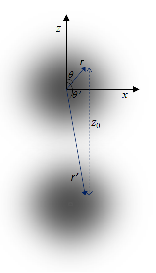
We have:
| (52) |
where ( being the gravity acceleration). The evaluation of is done again through numerical integration of Eq. (49). In the case of gravity fall we disregarded the effects related to thermal expansion.
The evaluation of the phase-shift for a cold sample of atoms in a cylindrical cavity in the cases of thermal expansion or gravity fall follows from analogous considerations.
For thermal atoms in a cylindrical cavity, the evaluation of the phase-shift according to the procedure here reported seems not applicable since the atomic motion is in this case totally random and in principle it is not possible to find any general relation between the positions assumed by the atoms during the two microwave pulses. However, to provide an order of magnitude for the phase-shift also in this case, we can make some approximations. First, as explained in the text, we are interested to the phase-variation along the -axis, so we suppose that all the atoms move either along the positive or negative direction of -axis. Owing to the randomness of the atomic motion, half of the cell volume ( in Eq. (53)) is occupied by atoms traveling in one direction and the other half by those moving in the opposite direction.
Under this approximation, the phase variations averaged over the cell volume becomes:
| (53) |
where we defined:
| (54) |
and
| (55) |
being the path traveled by the atoms during the Ramsey time along the positive direction of -axis and is given by Eq. (21). Analogous definitions hold for , , and .
Acknowledgements
The authors would like to thank Filippo Levi for useful discussions. This work has been funded by the EMRP programme (IND55 MClocks). The EMRP is jointly funded by the EMRP participating countries within EURAMET and the European Union.
References
- [1] A. Bauch, T. Heindorff, and R. Schroeder, Measurement of the Frequency-Shift Due to Distributed Cavity Phase Difference in an Atomic clock, IEEE. Trans. Instrum. Meas. 34, 136 (1985).
- [2] E. Bava, A. Godone, and C. Novero, Cavity phase-shift error evaluation in a magnesium atomic beam frequency standard, Appl. Phys. B 48, 495 (1989).
- [3] F. Chapelet, S. Bize, P. Wolf, G. Santarelli, P. Rosenbusch, M. E. Tobar, Ph. Laurent, C. Salomon, and A. Clairon, Invesigation of the distributed cavity phase shift in an atomic fountain, Proceedings of the 20th European Frequency and Time Forum, edited by F. Riehle, pp. 160-165, 2006.
- [4] S. Weyers, V. Gerginov, N. Nemitz, R. Li, and K. Gibble, Distributed cavity phase frequency shifts of the caesium fountain PTB-CSF2, Metrologia 49, 82 (2012).
- [5] R. Li, K. Gibble, and K. Szymaniec, Improved accuracy of the NPL-CsF2 primary frequency standard: evaluation of distributed cavity phase and microwave lensing frequency shifts, Metrologia 48, 283 (2011).
- [6] K. Szymaniec, S. E. Park, G. Marra, and W. Chalupczak, First accuracy evaluation of the NPL-Cs F2 primary frequency standard, Metrologia 47, 363 (2010).
- [7] J. Guena, P. Rosenbusch, Ph. Laurent, M. Abgrall, D. Rovera, G. Santarelli, M. E. Tobar, R. Li, K. Gibble, S. Bize, and A. Clairon, Characterization of the distributed cavity phase shift in FO2 for improving the accuracy of SYRTE fountain clocks, Proceedings of the 24th European Frequency and Time Forum, edited by P. Waller, pp. 1-7, 2010.
- [8] F. Levi, D. Calonico, C. E. Calosso, A. Godone, S. Micalizio, and G. A. Costanzo, Accuracy evaluation of ITCsF2: a nitrogen cooled caesium fountain, Metrologia 51, 270 (2014).
- [9] T. P. Heavner, E. A. Donley, F. Levi, G. A. Costanzo, T. E. Parker, J. H. Shirley, N. Ashby, S. Barlow, and S. R. Jefferts, Accuracy evaluation of ITCsF2: a nitrogen cooled caesium fountain, Metrologia 51, 174 (2014).
- [10] N. Ashby, S. Barlow, T. Heavner, S. Jefferts, Frequency shifts in NIST Cs primary frequency standards due to transverse rf field gradients, Phys. Rev. A 91, 033624 (2015).
- [11] G. Vecchi, and A. De Marchi, Spatial phase variations in a TE011 microwave cavity for use in cesium fountain primary frequency standard, IEEE Trans. Instrum. Meas. 42, 434 (1993).
- [12] A. Khursheed, G. Vecchi, A. De Marchi, Spatial variations of field polarization and phase in microwave cavities: application to the cesium fountain cavity, IEEE Trans. Ultrason. Ferroelect. Freq. Control 43, 201 (1996).
- [13] R. Li, and K. Gibble, Phase variations in microwave cavities for atomic clocks, Metrologia 41, 376 (2004).
- [14] R. Li, and K. Gibble, Evaluating and minimizing distributed cavity phase errors in atomic clocks, Metrologia 47, 534 (2010).
- [15] A. Godone, F. Levi, C. E. Calosso, and S. Micalizio, High-performing vapor-cell frequency standards, Rivista del Nuovo Cimento 38, 133 (2015).
- [16] S. Micalizio, C. E. Calosso, A. Godone, A and F.Levi, Metrological characterization of the pulsed Rb clock with optical detection, Metrologia 49, 425 (2012).
- [17] G. Mei, D. Zhong, S. An, F. Zhao, F. Qi, F. Wang, G. Ming, W. Li, P. Wang, Main Features of Space Rubidium Atomic Frequency Standard for BeiDou Satellites, Proceedings of the 30th European Frequency and Time Forum, p. 1, 2016.
- [18] S. T. Muller, D. V. Magalhaes, R. F. Alves, and V. S. Bagnato, Compact frequency standard based on an intracavity sample of cold cesium atoms, J. Opt. Soc. Am. B 28, 2592 (2011).
- [19] F.-X. Esnault, D. Holleville, N. Rossetto, S. Guerandel, and N. Dimarcq, Compact frequency standard based on an intracavity sample of cold cesium atoms, Phys. Rev. A 82, 033436 (2010).
- [20] L. De Sarlo, M. Langlois, D. Holleville, M. Lours, N. Dimarcq, J.-F. Schaff, S. Bernon, and B. Desruelle, Preliminary Test of a Cold-Atom Based Clock Prototype on a Microgravity Platform: Rubiclock on the a-300 0g, Proceedings of the 28th European Frequency and Time Forum, p. 1, 2014.
- [21] L. Peng, M. Yanling, W. Jinyin, W. Xiumei, W. Yaning, X. Ling, H. Cheng, L. Liang, Scheme for a compact cold-atom clock based on diffuse laser cooling in a cylindrical cavity, Phys. Rev. A 92, 062101 (2015).
- [22] H.-D. Cheng, W.-Z. Zhang, H.-Y. Ma, L. Liu, and Y.-Z. Wang, Laser cooling of rubidium atoms from background vapor in diffuse light, Phys. Rev. A 79, 023407 (2009).
- [23] N. Marcuvitz, Waveguide Handbook, P. Preregrinus Ltd., 1986.
- [24] R. E. Collin, Foundations for Microwave Engineering, McGraw-Hill, New York, 1966.
- [25] A. Godone, S. Micalizio, F. Levi, and C. Calosso, Microwave cavities for vapor cell frequency standards, Rev. Sci. Instrum. 82, 074703 (2011).
- [26] J. Vanier and C. Audoin, The Quantum Physics of Atomic Frequency Standards, Adam Hilger, Bristol, 1989.
- [27] J. A. Stratton, Electromagnetic Theory, McGraw-Hill, Cambridge, 1941.
- [28] J. A. Abramovitz and I. Stegun, Handbook of Mathematical Functions with Formulas, Graphs, and Mathematical Tables, National Bureau of Standards, Applied Mathematics Series, Vol. 55, 1964.
- [29] G. Santarelli, C. Audoin, A. Makdissi, Ph. Laurent, G. J. Dick, and A. Clairon, Frequency Stability Degradation of an Oscillator Slaved to a Periodically Interrogated Atomic Resonator, IEEE Trans. Ultrason. Ferroelect. Freq. Control 45, 887, 1998.
- [30] C. Audoin, G. Santarelli, A. Makdissi, and A. Clairon, Properties of an Oscillator Slaved to a Periodically Interrogated Atomic Resonator, IEEE Trans. Ultrason. Ferroelect. Freq. Control 45, 877 (1998).
- [31] G. J. Dick, Local oscillator induced instabilities in trapped ion frequency standards, Proceedings of the Precise Time and Time Interval Meeting (ed. Sydnor, R. L., US Naval Observatory), pp. 133-147, 1987.
- [32] Y.-L. Meng, H.-D. Cheng, B.-C. Zheng, X.-C. Wang, L. Xiao, and L. Liu, Controlling the Shape of a Cold Atom Cloud in a Cylindrical Cavity, Chin. Phys. Lett. 30, 063701 (2013).
- [33] X.-C. Wang, H.-D. Cheng, L. Xiao, B.-C. Zheng, Y.-L. Meng, L. Liu, and Y.-Z. Wang, Measurement of Spatial Distribution of Cold Atoms in an Integrating Sphere, Chin. Phys. Lett. 29, 023701 (2012).
- [34] F.-X. Esnault, S. Perrin, D. Holleville, S. Guerandel, N. Dimarcq, N and J. Delporte, Stability of the compact cold atom clock HORACE, IEEE International Frequency Control Symposium, 2007 Joint with the 21st European Frequency and Time Forum, 28th May- 1st June, Geneva, p. 1342, 2007.