跳到论文正文
W Papers独立论文阅读器 arXiv:1705.00586 论文正文 计算阅读时间 · 0%
引用这篇论文根据当前论文元数据生成,正式投稿前建议核对。


License: arXiv.org perpetual non-exclusive license
arXiv:1705.00586v4 [math.ST] 29 May 2017

Bootstrap confidence bands for spectral estimation of Lévy densities under high-frequency observationsThanks: K. Kato is supported by Grant-in-Aid for Scientific Research (C) (15K03392) from the JSPS. D. Kurisu is supported by Grant-in-Aid for JSPS Research Fellow (16J06454) from the JSPS. We would like to thank Yuya Sasaki for kindly sharing the codes.

Kengo Kato K. Kato Graduate School of Economics, University of Tokyo
7-3-1 Hongo, Bunkyo-ku, Tokyo 113-0033, Japan.
Email address: kkato@e.u-tokyo.ac.jp
and Daisuke Kurisu D. Kurisu Graduate School of Economics, University of Tokyo
7-3-1 Hongo, Bunkyo-ku, Tokyo 113-0033, Japan.
Email address: dkurisu.mathstat@gmail.com
Date: First version: May 1, 2017. This version: August 24, 2026
Abstract.

This paper develops bootstrap methods to construct uniform confidence bands for nonparametric spectral estimation of Lévy densities under high-frequency observations. We assume that we observe nn discrete observations at frequency 1/Δ>01/\Delta>0, and work with the high-frequency setup where Δ=Δn→0\Delta=\Delta_{n}\to 0 and n​Δ→∞n\Delta\to\infty as n→∞n\to\infty. We employ a spectral (or Fourier-based) estimator of the Lévy density, and develop novel implementations of Gaussian multiplier (or wild) and empirical (or Efron’s) bootstraps to construct confidence bands for the spectral estimator on a compact set that does not intersect the origin. We provide conditions under which the proposed confidence bands are asymptotically valid. Our confidence bands are shown to be asymptotically valid for a wide class of Lévy processes. We also develop a practical method for bandwidth selection, and conduct simulation studies to investigate the finite sample performance of the proposed confidence bands.

Key words and phrases: 
empirical bootstrap, high-frequency data, Lévy process, multiplier bootstrap, spectral estimation

1. Introduction

In the financial economics literature, it has been argued that the presence of jumps plays an important role in the dynamics of financial data such as asset returns, interest rates, currencies, and so on (Cont and Tankov, 2004; Aït-Sahalia, 2004; Johannes, 2004; Aït-Sahalia and Jacod, 2014, cf.). For example, Johannes (2004) studies the dynamics of interest rate movements and argues that the presence of jumps contributes to capturing non-normalities of increment distributions that are consistent with empirical data but diffusion models can not capture. A Lévy process is a fundamental class of continuous-time stochastic processes allowing for jumps; we refer to Sato (1999) and Bertoin (1996) as standard references on Lévy processes. From the Lévy-Itô decomposition (Sato, 1999, Theorem 19.2), a Lévy process is decomposed into the sum of drift, Brownian, and jump components, and the distribution of the Lévy process is completely determined by the three parameters, namely, the drift, the diffusion coefficient, and the Lévy measure. The Lévy measure controls the jump dynamics of the Lévy process, and therefore, inference on the Lévy measure is of particular interest. In this paper, we assume that the Lévy density has a Lebesgue density (Lévy density), and study inference on the Lévy density from high-frequency observations. High-frequency data – data collected for every minute, second, or even microsecond – have become available due to the advancement of information technologies, and the analysis of high-frequency financial data has attracted a great deal of attentions in the financial econometrics literature; see, e.g., Aït-Sahalia and Jacod (2014).

To be precise, we work with the following setting. Let L=(Lt)t≥0L=(L_{t})_{t\geq 0} be a Lévy process, i.e., LL is a stochastic process starting at 00 with stationary independent increments and càdlàg sample paths. From the Lévy-Khinchin representation (Sato, 1999, Theorem 8.1), LtL_{t} has characteristic function φt​(u)=E⁡[ei​u​Lt]=et​ψ​(u),u∈ℝ\varphi_{t}(u)=\mathrm{E}[e^{iuL_{t}}]=e^{t\psi(u)},u\in\mathbb{R}, where i=−1i=\sqrt{-1}, and

ψ⁡(u)=−u2​σ22+i​u​γ+∫ℝ(ei​u​x−1−i​u​x​1[−1,1]​(x))​ν​(𝑑x).\psi(u)=-\frac{u^{2}\sigma^{2}}{2}+iu\gamma+\int_{\mathbb{R}}(e^{iux}-1-iux1_{[-1,1]}(x))\nu(dx).

The triplet (σ2,γ,ν)(\sigma^{2},\gamma,\nu), called the Lévy triplet, completely characterizes the distribution of the Lévy process LL (cf. Sato, 1999, Theorem 7.10). Specifically, σ2≥0\sigma^{2}\geq 0 is the diffusion coefficient, γ∈ℝ\gamma\in\mathbb{R} is the drift, and ν\nu is the Lévy measure, i.e., a Borel measure on ℝ\mathbb{R} such that

∫ℝ(1∧x2)​ν​(𝑑x)<∞andν⁡({0})=0.\int_{\mathbb{R}}(1\wedge x^{2})\nu(dx)<\infty\quad\text{and}\quad\nu(\{0\})=0.

For any (Borel) set A⊂ℝA\subset\mathbb{R}, ν⁡(A)\nu(A) coincides with the expected number of jumps falling in A∖{0}A\setminus\{0\} in the unit time:

ν⁡(A)=E⁡[∑0<t≤11​(Lt−Lt−∈A∖{0})],\nu(A)=\mathrm{E}\left[\sum_{0<t\leq 1}1(L_{t}-L_{t-}\in A\setminus\{0\})\right],

where Lt−=lims↑tLsL_{t-}=\lim_{s\uparrow t}L_{s} (recall that LL has at most countably many jumps on (0,t](0,t] for any t>0t>0). In this paper, we assume that the Lévy measure has Lebesgue density ρ\rho, called the Lévy density, i.e., ν⁡(d​x)=ρ⁡(x)​d​x\nu(dx)=\rho(x)dx. Furthermore, we assume that we observe discrete observations Lj​Δ,j=1,…,nL_{j\Delta},\ j=1,\dots,n at frequency 1/Δ>01/\Delta>0, and work with the high-frequency setup where Δ=Δn→0\Delta=\Delta_{n}\to 0 and n​Δ→∞n\Delta\to\infty as n→∞n\to\infty. Since we are interested in estimation of the Lévy measure (or more precisely its Lebesgue density), we require n​Δ→∞n\Delta\to\infty. Heuristically, this can be understood from the observation that, within any fixed time interval, say the unit time, the Lévy process (Lt)t∈[0,1](L_{t})_{t\in[0,1]} has only finitely many jumps that fall in a local neighborhood not containing the origin, so that even if the whole path (Lt)t∈[0,1](L_{t})_{t\in[0,1]} could be observed, there are only finitely many data that can be used to estimate the Lévy measure at the local neighborhood. Concretely, we have in mind that the unit time is one day, and if we have 6.5 trading hours in a day and take 5 minutes as a time span, then Δ=5/(6.5×60)=1/78≈0.013\Delta=5/(6.5\times 60)=1/78\approx 0.013; each year has around 252 business days, and so we have 78×252=1965678\times 252=19656 observations per a year.

Under this setup, the goal of this paper is to develop bootstrap methods to construct confidence bands for the Lévy density. Since the Lévy density can blow up around the origin, we focus on confidence bands on a compact set that does not intersect the origin. We employ a spectral (or Fourier-based) estimator of the Lévy density, and develop novel implementations of Gaussian multiplier and empirical bootstraps to construct confidence bands for the spectral estimator. We provide conditions under which the proposed confidence bands are asymptotically valid. Notably, our confidence bands are shown to be asymptotically valid for a wide class of Lévy processes, including compound Poisson processes, (Variance-) Gamma processes, Inverse Gaussian processes, tempered stable processes, and Normal Inverse Gaussian processes with or without Brownian components.11 1 For tempered stable processes, however, the stability index has is at most 11 for a technical reason. Confidence bands provide a simple graphical description of the accuracy of a nonparametric curve estimator, thereby quantifying uncertainties of the estimator simultaneously over (in most cases continuum of) designs points, which is of practical importance in statistical analysis. Despite extensive studies on consistent estimation of the Lévy density, however, research on confidence intervals or bands for the Lévy density is relatively scarce – see a literature review below. In particular, to the best of our knowledge, this is the first paper to derive bootstrap-based confidence bands for the Lévy density. In addition to the theoretical results, we also develop a practical method for bandwidth selection, inspired by Bissantz et al. (2007), and conduct simulation studies to investigate the finite sample performance of the proposed confidence bands.

The literature on nonparametric estimation of Lévy measures or densities is broad. Recent contributions include Shimizu (2006), Figueroa-López (2009), Comte and Genon-Catalot (2009); Comte and Genon-Catalot (2010); Comte and Genon-Catalot (2015), Kappus and Reiß (2010), Duval (2013), and Bec and Lacour (2015) under the high-frequency setup (i.e., Δ=Δn→0\Delta=\Delta_{n}\to 0 as n→∞n\to\infty), and van Es et al. (2007), Neumann and Reiß (2009), Gugushvili (2009), Chen et al. (2010), Comte and Genon-Catalot (2010), Kappus and Reiß (2010), Belomestny (2011), Gugushvili (2012), Kappus (2014), Trabs (2015), and Belomestny and Reiß (2015) under the low-frequency setup (i.e., Δ>0\Delta>0 is fixed). Jongbload et al. (2005) study nonparametric estimation of the Lévy measure for a Lévy driven Ornstein-Uhlenbeck process under high and low frequency observations. Nickl and Reiß (2012) and Nickl et al. (2016) study estimation of distribution functions such as ∫−∞⋅(1∧x2)​ν​(𝑑x)\int_{-\infty}^{\cdot}(1\wedge x^{2})\nu(dx), and prove Donsker-type functional limit theorems for distributional function estimators under low- and high-frequency setups, respectively. We also refer to Bücher and Vetter (2013), Vetter (2014), Bücher et al. (2017), and Hoffmann and Vetter (2017) for inference on Lévy measures. However, none of these papers studies confidence bands for Lévy densities.

To the best of our knowledge, Figueroa-López (2011b) and its follow-up paper Konakov and Panov (2016) are the only references that derive uniform confidence bands for Lévy densities. They work with the high-frequency setup, but employ sieve (or projection) estimators based on the observation that Δ−1​P​(LΔ≥x)≈ν⁡([x,∞))\Delta^{-1}\mathrm{P}(L_{\Delta}\geq x)\approx\nu([x,\infty)) for x>0x>0 (Figueroa-López, 2009, see also), which are substantially different from our spectral estimator. So, first of all, their results do not cover ours. Similarly to Smirnov (1950) and Bickel and Rosenblatt (1973), Figueroa-López (2011b) proves that the supremum deviation of the sieve estimator, suitably normalized, converges in distribution to a Gumbel distribution, by using the Komlós-Major-Tusnády (KMT) approximation of the empirical distribution function by Brownian bridges (Komlós et al., 1975), combined with extreme value theory. Figueroa-López (2011b) uses the Gumbel approximation to construct analytic confidence bands for the Lévy density, but does not study bootstrap-based confidence bands. However, since the convergence of normal extremes is known to be slow (Hall, 1991), in standard nonparametric density and regression function estimation, it is often recommended to use versions of bootstraps to construct confidence bands, instead of relying on Gumbel approximations (Neumann and Polzeh;, 1998; Claeskens and Van Keilegom, 2003; Chernozhukov et al., 2014a, cf.).22 2 For the trigonometric basis, Konakov and Panov (2016) develop an analytical method based on higher oder expansions to improve on the Gumbel approximation; see their Theorem 3.7. This paper contributes to the literature on nonparametric inference for Lévy processes by developing bootstrap confidence bands for the first time in the Lévy density estimation case. Furthermore, spectral-type estimators are among the most commonly used methods for estimation of the Lévy density (Comte and Genon-Catalot, 2015; Belomestny and Reiß, 2015, cf.), and developing inference methods for them is practically important.

From a technical point of view, the proofs of the main theorems build on non-trivial applications of the intermediate Gaussian and bootstrap approximation theorems developed in Chernozhukov et al. (2014a); Chernozhukov et al. (2014b); Chernozhukov et al. (2016). The analysis of the present paper has some connections to those of Kato and Sasaki (2016); Kato and Sasaki (2017) that study confidence bands for deconvolution and nonparametric errors-in-variables regression, respectively. However, the high-frequency setup in Lévy process estimation has different probabilistic structures than the i.i.d. setup in standard nonparametric estimation. For example, the increment distribution PΔP_{\Delta} (i.e., the distribution of LΔL_{\Delta}) need not be continuous and may have a discrete component (which is in contrast to the standard density estimation case); PΔP_{\Delta} is indexed by Δ\Delta with Δ=Δn→0\Delta=\Delta_{n}\to 0 as n→∞n\to\infty, and degenerates to the point mass at the origin; and the interplay between Δ\Delta and nn has to be taken care of. In particular, providing low-level regularity conditions for validity of bootstrap confidence bands in the Lévy density estimation case is far from trivial and requires substantial work. See the discussion after Assumption 4.1 and Section 4.2.

In this paper, we assume that data do not contain microstructure noises. We have in mind that the time span Δ\Delta is small but not too small – say 5 minutes if the unit time is one day. For such cases, Aït-Sahalia and Xiu (2017) argue that the effect of microstructure noise is small.

The rest of the paper is organized as follows. In Section 2, we define a spectral estimator for the Lévy density, and in Section 3 we describe our bootstrap methods to construct confidence bands for the spectral estimator. We consider two bootstrap methods, namely, Gaussian multiplier and empirical bootstraps. In Section 4, we present theorems that establish asymptotic validity of the proposed confidence bands. In Section 5, we provide concrete examples of Lévy processes that satisfy our regularity conditions. In Section 6, we propose a practical method for bandwidth selection, and study its finite sample performance via numerical simulations. Section 7 concludes. All the proofs are deferred to Appendix.

1.1. Notation

We will obey the following notation. For any non-empty set TT and any (complex-valued) function ff on TT, let ‖f‖T=supt∈T|f⁡(t)|\|f\|_{T}=\sup_{t\in T}|f(t)|. Let ℓ∞​(T)\ell^{\infty}(T) denote the (real) Banach space of all bounded real-valued functions on TT equipped with the sup-norm ∥⋅∥T\|\cdot\|_{T}. The Fourier transform of an integrable function ff on ℝ\mathbb{R} is defined as

φf​(u)=∫ℝei​u​x​f​(x)​𝑑x,u∈ℝ.\varphi_{f}(u)=\int_{\mathbb{R}}e^{iux}f(x)dx,\ u\in\mathbb{R}.

For any x∈ℝx\in\mathbb{R}, let δx\delta_{x} denote the Dirac measure at xx. For any a,b∈ℝa,b\in\mathbb{R}, let a∨b=max⁡{a,b}a\vee b=\max\{a,b\} and a∧b=min⁡{a,b}a\wedge b=\min\{a,b\}. For a∈ℝa\in\mathbb{R} and b>0b>0, we use the shorthand notation [a±b]=[a−b,a+b][a\pm b]=[a-b,a+b]. For any non-empty set AA in ℝ\mathbb{R} and any ε>0\varepsilon>0, let Aε={x∈ℝ:d⁡(x,A)≤ε}A^{\varepsilon}=\{x\in\mathbb{R}:d(x,A)\leq\varepsilon\} where d⁡(x,A)=infy∈A|x−y|d(x,A)=\inf_{y\in A}|x-y|. For any positive sequences an,bna_{n},b_{n}, we write an≲bna_{n}\lesssim b_{n} if there is a positive constant C>0C>0 independent of nn such that an≤C​bna_{n}\leq Cb_{n} for all nn, an∼bna_{n}\sim b_{n} if an≲bna_{n}\lesssim b_{n} and bn≲anb_{n}\lesssim a_{n}, and an≪bna_{n}\ll b_{n} if an/bn→0a_{n}/b_{n}\to 0 as n→∞n\to\infty.

2. Spectral estimation of Lévy density

We first describe a spectral estimation method for Lévy densities. Let Yn,j=Lj​Δ−L(j−1)​Δ,j=1,…,nY_{n,j}=L_{j\Delta}-L_{(j-1)\Delta},j=1,\dots,n be increments of discrete observations of the Lévy process LL, and observe that Yn,j,j=1,…,nY_{n,j},j=1,\dots,n are i.i.d. whose common characteristic function is φΔ​(u)=E⁡[ei​u​LΔ]=eΔ​ψ​(u)\varphi_{\Delta}(u)=\mathrm{E}[e^{iuL_{\Delta}}]=e^{\Delta\psi(u)}. In this paper, we assume that

∫ℝx2​ρ​(x)​𝑑x<∞,\int_{\mathbb{R}}x^{2}\rho(x)dx<\infty, (2.1)

which is equivalent to assuming that E⁡[L12]<∞\E[L_{1}^{2}]<\infty (and E⁡[Lt2]<∞\mathrm{E}[L_{t}^{2}]<\infty for all t>0t>0; see Sato (1999), Corollary 25.8). Condition (2.1) ensures that the integral ∫ℝ(ei​u​x−1−i​u​x)​ρ​(x)​𝑑x\int_{\mathbb{R}}(e^{iux}-1-iux)\rho(x)dx is well-defined, so that the characteristic exponent ψ⁡(u)\psi(u) admits an alternative representation:

ψ⁡(u)=−u2​σ22+i​u​γc+∫ℝ(ei​u​x−1−i​u​x)​ρ​(x)​𝑑x,\psi(u)=-\frac{u^{2}\sigma^{2}}{2}+iu\gamma_{c}+\int_{\mathbb{R}}(e^{iux}-1-iux)\rho(x)dx,

where γc=i−1​(eψ⁡(u))′|u=0=E⁡[L1]\gamma_{c}=i^{-1}(e^{\psi(u)})^{\prime}|_{u=0}=\mathrm{E}[L_{1}]. Furthermore, under Condition (2.1), differentiating ψ⁡(u)\psi(u) twice, we arrive at the key identity

ψ′′​(u)=φΔ′′​(u)​φΔ​(u)−(φΔ′​(u))2Δ​φΔ2​(u)=−σ2−∫ℝei​u​x​x2​ρ​(x)​𝑑x.\psi^{\prime\prime}(u)={\varphi^{\prime\prime}_{\Delta}(u)\varphi_{\Delta}(u)-(\varphi^{\prime}_{\Delta}(u))^{2}\over\Delta\varphi_{\Delta}^{2}(u)}=-\sigma^{2}-\int_{\mathbb{R}}e^{iux}x^{2}\rho(x)dx.

Therefore, applying the Fourier inversion, we conclude that

x2​ρ​(x)\displaystyle x^{2}\rho(x) =12​π​∫ℝe−i​u​x​(−ψ′′​(u)−σ2)​𝑑u\displaystyle={1\over 2\pi}\int_{\mathbb{R}}e^{-iux}\left(-\psi^{\prime\prime}(u)-\sigma^{2}\right)du
=12​π​∫ℝe−i​u​x​((φΔ′​(u))2−φΔ′′​(u)​φΔ​(u)Δ​φΔ2​(u)−σ2)​𝑑u,\displaystyle={1\over 2\pi}\int_{\mathbb{R}}e^{-iux}\left({(\varphi^{\prime}_{\Delta}(u))^{2}-\varphi^{\prime\prime}_{\Delta}(u)\varphi_{\Delta}(u)\over\Delta\varphi^{2}_{\Delta}(u)}-\sigma^{2}\right)du, (2.2)

where the Fourier inversion should be interpreted in the distributional sense if the integral is not well-defined. This expression leads to a method to estimate ρ\rho.

First, we estimate φΔ(k)​(u),k=0,1,2\varphi_{\Delta}^{(k)}(u),k=0,1,2 by φ^Δ(k)​(u)\widehat{\varphi}_{\Delta}^{(k)}(u), where

φ^Δ​(u)=1n​∑j=1nei​u​Yn,j,u∈ℝ\widehat{\varphi}_{\Delta}(u)=\frac{1}{n}\sum_{j=1}^{n}e^{iuY_{n,j}},\ u\in\mathbb{R}

is the empirical characteristic function (φΔ(k)\varphi_{\Delta}^{(k)} denotes the kk-th derivative of φΔ\varphi_{\Delta} with φΔ(0)=φΔ\varphi_{\Delta}^{(0)}=\varphi_{\Delta}). Let W:ℝ→ℝW:\mathbb{R}\to\mathbb{R} be an integrable function (kernel) such that ∫ℝW⁡(x)​𝑑x=1\int_{\mathbb{R}}W(x)dx=1 and its Fourier transform φW\varphi_{W} is supported in [−1,1][-1,1] (i.e., φW​(u)=0\varphi_{W}(u)=0 for all |u|>1|u|>1). Then the spectral estimator of ρ\rho is defined by

ρ^​(x)=12​π​x2​∫ℝe−i​u​x​((φ^Δ′​(u))2−φ^Δ′′​(u)​φ^Δ​(u)Δ​φ^Δ2​(u)−σ^2)​φW​(u​h)​𝑑u\widehat{\rho}(x)={1\over 2\pi x^{2}}\int_{\mathbb{R}}e^{-iux}\left({(\widehat{\varphi}^{\prime}_{\Delta}(u))^{2}-\widehat{\varphi}^{\prime\prime}_{\Delta}(u)\widehat{\varphi}_{\Delta}(u)\over\Delta\widehat{\varphi}^{2}_{\Delta}(u)}-\widehat{\sigma}^{2}\right)\varphi_{W}(uh)du (2.3)

for x≠0x\neq 0, where h=hnh=h_{n} is a sequence of positive numbers (bandwidths) such that hn→0h_{n}\to 0 as n→∞n\to\infty, and σ^2\widehat{\sigma}^{2} is a pilot estimator of σ2\sigma^{2}.

Some comments on the spectral estimator ρ^\widehat{\rho} are in order. First, as long as h≳Δ1/2h\gtrsim\Delta^{1/2}, inf|u|≤h−1|φ^Δ​(u)|≳1−oP​(1)\inf_{|u|\leq h^{-1}}|\widehat{\varphi}_{\Delta}(u)|\gtrsim 1-o_{\mathrm{P}}(1), so that ρ^​(x)\widehat{\rho}(x) for x≠0x\neq 0 is well-defined with probability approaching one (see Lemmas A.2 and A.4). Second, the function ρ^\widehat{\rho} is real-valued. Third, noting that ψ^:=Δ−1​log⁡φ^Δ\widehat{\psi}:=\Delta^{-1}\log\widehat{\varphi}_{\Delta} is well-defined on [−h−1,h−1][-h^{-1},h^{-1}] (with probability approaching one) as the distinguished logarithm (Chung, 2001, Theorem 7.6.2), we see that the spectral estimator ρ^\widehat{\rho} can be alternatively expressed as

ρ^​(x)=12​π​x2​∫ℝe−i​u​x​(−ψ^′′​(u)−σ^2)​φW​(u​h)​𝑑u\widehat{\rho}(x)=\frac{1}{2\pi x^{2}}\int_{\mathbb{R}}e^{-iux}\left(-\widehat{\psi}^{\prime\prime}(u)-\widehat{\sigma}^{2}\right)\varphi_{W}(uh)du

for x≠0x\neq 0. Finally, in this paper, we are interested in estimating ρ\rho on a compact set II away from the origin (e.g. [a,b]∪[c,d][a,b]\cup[c,d] for a<b<0<c<da<b<0<c<d), and therefore, as long as |W⁡(x)||W(x)| decays sufficiently fast as |x|→∞|x|\to\infty, we may take σ^2=0\widehat{\sigma}^{2}=0 in theory. See the discussion after Assumption 4.1 below. However, in our simulation studies, we found that, in case of σ>0\sigma>0, using a proper estimator for σ^2\widehat{\sigma}^{2} improves on the empirical performance of the estimator ρ^\widehat{\rho} and the inference methods, especially if the set II is close to the origin. Therefore, we recommend to plug-in a proper estimator of σ2\sigma^{2}. There are several existing estimators for σ2\sigma^{2}; see Example 2.1 below.

Our spectral estimator (2.3) is considered and studied in Belomestny (2011) and Gugushvili (2012) under the low-frequency setup. Nickl et al. (2016) use the spectral estimator (2.3) to construct estimators for distribution functions such as ∫−∞⋅(1∧x2)​ν​(𝑑x)\int_{-\infty}^{\cdot}(1\wedge x^{2})\nu(dx), and prove Donsker-type functional limit theorems for distribution function estimators under the high-frequency setup. There are versions of spectral-type estimators of ρ\rho similar to but different from ours (2.3). For example, in case of σ=0\sigma=0, Comte and Genon-Catalot (2011) consider simplified versions of the estimator (2.3) by replacing φ^Δ​(u)\widehat{\varphi}_{\Delta}(u) with 1 and/or φ^Δ′​(u)\widehat{\varphi}_{\Delta}^{\prime}(u) with 00. Such simplifications produce additional biases that depend on Δ\Delta (but not on smoothness of x2​ρx^{2}\rho); since the problem of bias is already delicate in construction of confidence bands in standard nonparametric estimation (cf. Wasserman, 2006, Section 5.7), producing additional biases is not favorable to our goal from both theoretical and practical view points. Hence, in this paper, we focus on the current spectral estimator (2.3). It is worth pointing out that the identification (2.2) of the Lévy density ρ\rho holds without relying on the assumption that Δ→0\Delta\to 0, and therefore the deterministic bias of our spectral estimator ρ^\widehat{\rho} does not depend on Δ\Delta; see the discussion after Assumption 4.1 below.

Furthermore, under relatively mild conditions, our spectral estimator (2.3) is consistent under the weighted sup-norm on ℝ\mathbb{R}, ‖f‖w,∞=supx∈ℝ|x2​f​(x)|\|f\|_{w,\infty}=\sup_{x\in\mathbb{R}}|x^{2}f(x)| (see Appendix C), and thereby is able to capture the shape of ρ\rho globally (i.e., uniformly over ℝ∖{0}\mathbb{R}\setminus\{0\}), which we believe is an attractive feature of the spectral estimator ρ^\widehat{\rho}.

Example 2.1 (Examples of estimators for σ2\sigma^{2}).

There are several consistent estimators for σ2\sigma^{2} available in the literature on high-frequency data analysis for continuous-time stochastic processes. We provide a couple of examples here. The first example is the truncated realized volatility (TRV) estimator proposed in Mancini (2001) :

σ^2T​R​V=1n​Δ∑j=1nYn,j21{|Yn,j|≤α0Δθ0},\widehat{\sigma}^{2}_{TRV}={1\over n\Delta}\sum_{j=1}^{n}Y_{n,j}^{2}1_{\{|Y_{n,j}|\leq\alpha_{0}\Delta^{\theta_{0}}\}}, (2.4)

where α0>0\alpha_{0}>0 and θ0∈(0,1/2)\theta_{0}\in(0,1/2). The second example is the power variation (PV) estimator proposed in Barndorff-Nielsen and Shephard (2004):

σ^P​V2​(α)=(1n​Δα/2​mα​∑j=1n|Yn,j|α)2/α,\widehat{\sigma}^{2}_{PV}(\alpha)=\left({1\over n\Delta^{\alpha/2}m_{\alpha}}\sum_{j=1}^{n}|Y_{n,j}|^{\alpha}\right)^{2/\alpha},

where α∈(0,2)\alpha\in(0,2) and mα=2α/2​Γ​((α+1)/2)/πm_{\alpha}=2^{\alpha/2}\Gamma((\alpha+1)/2)/\sqrt{\pi} is the α\alpha-th absolute moment of N⁡(0,1)N(0,1). Jacod and Reiß (2014) study the optimal rate of convergence for estimating σ2\sigma^{2} in the minimax sense and propose the following estimator (modified to our setup):

σ^J​R2=−2Δ​un2(log|φ^Δ(un)|)1{φ^Δ(un)≠0},\widehat{\sigma}^{2}_{JR}=-{2\over\Delta u_{n}^{2}}(\log|\widehat{\varphi}_{\Delta}(u_{n})|)1_{\{\widehat{\varphi}_{\Delta}(u_{n})\neq 0\}},

where un∝(log⁡n)/Δu_{n}\propto\sqrt{(\log n)/\Delta} is a deterministic sequence. In our simulation studies, we use σ^T​R​V2\widehat{\sigma}^{2}_{TRV} as an estimator of σ2\sigma^{2}.

Strictly speaking, the references cited above study the asymptotic properties of the estimators under a different high-frequency setup that Δ→0\Delta\to 0 as n→∞n\to\infty but n​Δn\Delta is fixed. For the asymptotic properties of the PV and JR estimators under our setup, we refer to Comte and Genon-Catalot (2011, Proposition 5.3) (Aït-Sahalia and Jacod, 2007, see also) and Nickl et al. (2016, Proposition 13), respectively. For the sake of completeness, we summarize the asymptotic properties of the TRV estimator in the following lemma. See Appendix B.1 for the proof.

Lemma 2.1.

Suppose that the Lévy measure satisfies ∫[−1,1]|x|α​ν​(𝑑x)<∞\int_{[-1,1]}|x|^{\alpha}\nu(dx)<\infty for some α∈(0,2)\alpha\in(0,2), and if α∈[1,2)\alpha\in[1,2), then assume in addition that ∫[−1,1]c|x|​ν​(𝑑x)<∞\int_{[-1,1]^{c}}|x|\nu(dx)<\infty. Then |σ^T​R​V2−σ2|=OP(n−1/2+Δ(2−α)​θ0)|\widehat{\sigma}^{2}_{TRV}-\sigma^{2}|=O_{\mathrm{P}}(n^{-1/2}+\Delta^{(2-\alpha)\theta_{0}}).

2.1. Comparison with direct kernel estimation: preliminary simulations

Alternatively to spectral-type estimation methods, exploiting the assumption that Δ→0\Delta\to 0 as n→∞n\to\infty, we can estimate the Lévy density ρ⁡(x)\rho(x) for x≠0x\neq 0 by applying directly kernel density estimation to increments Yn,1,…,Yn,nY_{n,1},\dots,Y_{n,n}, i.e.,

ρ^d​i​r​e​c​t​(x)=1n​Δ​h​∑j=1nWd​i​r​e​c​t​((x−Yn,j)/h),\widehat{\rho}^{direct}(x)=\frac{1}{n\Delta h}\sum_{j=1}^{n}W^{direct}((x-Y_{n,j})/h), (2.5)

where Wd​i​r​e​c​t:ℝ→ℝW^{direct}:\mathbb{R}\to\mathbb{R} is a compactly supported smooth kernel function. In fact, for a given fixed x≠0x\neq 0, if ρ\rho is Lipschitz continuous in a neighborhood of xx, then from Lemma B.1 and Proposition 2.1 in Figueroa-López (2011b), we can show that

E⁡[ρ^d​i​r​e​c​t​(x)]=1h​∫ℝWd​i​r​e​c​t​((x−y)/h)​ρ​(y)​dy⏟=ρ⁡(x)+O⁡(h)+O⁡(Δ/h),\mathrm{E}[\widehat{\rho}^{direct}(x)]=\underbrace{\frac{1}{h}\int_{\mathbb{R}}W^{direct}((x-y)/h)\rho(y)dy}_{=\rho(x)+O(h)}+O(\Delta/h),

so that ρ^d​i​r​e​c​t\widehat{\rho}^{direct} is consistent for ρ\rho at xx under appropriate regularity conditions. Actually, the direct kernel estimator (2.5) is mentioned in Figueroa-Löpez (2011a, Section 4.1), although the detailed properties of (2.5) are not studied there. From a theoretical point of view, it is rather easier to develop inference methods for ρ^d​i​r​e​c​t\widehat{\rho}^{direct} than the spectral estimator (2.3) under the high-frequency setup, since the former is of simpler form than the latter. So, one might be tempted to wonder why we bother to use a more complicated estimator ρ^\widehat{\rho}.

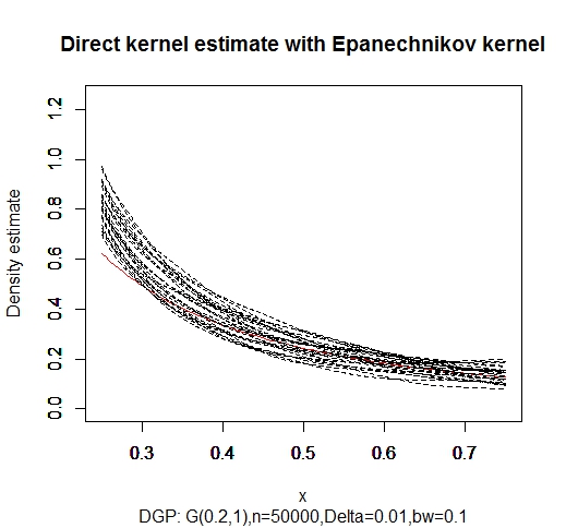
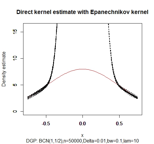
It turns out that, however, in the finite sample, the direct kernel estimate (2.5) tends to have (much) larger biases, especially near the origin, than the spectral estimate (2.3). Figures 1 and 2 compare realizations of direct kernel estimates with Epanechnikov kernel and spectral estimates with a flap-top kernel for a jump-diffusion process Lt=Bt+JtL_{t}=B_{t}+J_{t} where B=(Bt)t≥0B=(B_{t})_{t\geq 0} is a standard Brownian motion and J=(Jt)t≥0J=(J_{t})_{t\geq 0} is a compound Poisson process (independent of BB) with intensity λ=10\lambda=10 and jump size distribution N⁡(0,v2)N(0,v^{2}) (v=0.5v=0.5), and for a Gamma process with parameter (c+,λ+)=(0.2,1)(c_{+},\lambda_{+})=(0.2,1) (i.e, LΔL_{\Delta} has Gamma distribution with shape parameter c+​Δc_{+}\Delta and scale parameter 11). Here we set (n,Δ)=(50000,0.01)(n,\Delta)=(50000,0.01). Preliminary calibrations show that h=Δ=0.1h=\sqrt{\Delta}=0.1 works well for for both estimates, and we set this bandwidth value to generate these figures. The flap-top kernel used for the spectral estimate is defined by the inverse Fourier transform of equation (4.4) ahead with b=1b=1 and c=0.05c=0.05. Furthermore, for the spectral estimate, we plug-in the TRV estimate σ^T​R​V2\widehat{\sigma}^{2}_{TRV} with α0=3\alpha_{0}=3 and θ0=0.48\theta_{0}=0.48 for the jump-diffusion case, and set σ^2=0\widehat{\sigma}^{2}=0 for the Gamma process case (using the TRV estimate for the Gamma process case produced almost same simulation results).
Refer to caption Refer to caption
Figure 1. Plots of 25 realizations of direct kernel estimates with Epanechnikov kernel (left) and spectral estimates with a flap-top kernel (right) on [−0.75,−0.25]∪[0.25,0.75][-0.75,-0.25]\cup[0.25,0.75] for Lt=Bt+JtL_{t}=B_{t}+J_{t} where BtB_{t} is a standard Brownian motion and JtJ_{t} is a compound Poisson process with intensity λ=10\lambda=10 and jump size distribution N⁡(0,v2)N(0,v^{2}) (v=0.5v=0.5). The bandwidth value is h=Δ=0.1h=\sqrt{\Delta}=0.1. The red lines correspond to the true Lévy density ρ(x)=λe−x2/(2v2)/2​π​v2\rho(x)=\lambda e^{-x^{2}/(2v^{2})}/\sqrt{2\pi v^{2}}.
Refer to caption Refer to caption
Figure 2. Plots of 25 realizations of direct kernel estimates with Epanechnikov kernel (left) and spectral estimates with a flap-top kernel (right) on [0.25,0.75][0.25,0.75] where LtL_{t} is a Gamma process with parameter (c+,λ+)=(0.2,1)(c_{+},\lambda_{+})=(0.2,1), i.e., LΔL_{\Delta} has Gamma distribution with shape parameter c+​Δc_{+}\Delta and scale parameter λ+\lambda_{+}. The bandwidth value is h=Δ=0.1h=\sqrt{\Delta}=0.1. The red lines correspond to the true Lévy density ρ⁡(x)=c+​x−1​e−λ+​x​1(0,∞)​(x)\rho(x)=c_{+}x^{-1}e^{-\lambda_{+}x}1_{(0,\infty)}(x).

These figures show that the direct kernel estimate has large biases especially near the origin, whereas the spectral estimate performs reasonably well on the entire set for each case ([−0.75,−0.25]∪[0.25,0.75][-0.75,-0.25]\cup[0.25,0.75] for the jump-diffusion case, and [0.25,0.75][0.25,0.75] for the Gamma process case). In particular, the direct kernel estimate exhibits unreasonable behaviors for |x|<0.5|x|<0.5 in the jump-diffusion case. Intuitively, such unreasonable behaviors can be understood from the observation that the increment distribution PΔP_{\Delta} (i.e., the distribution of LΔL_{\Delta}) of the jump-diffusion process is the convolution of N⁡(0,Δ​v2)N(0,\Delta v^{2}) with the compound Poisson distribution that has a point mass at the origin, and therefore, the density of PΔP_{\Delta} has a sharp peak around the origin. Since the direct kernel estimate is estimating the density of PΔP_{\Delta} scaled by Δ−1\Delta^{-1}, it tends to return unreasonably large values near the origin (we also note that, since P⁡(|N⁡(0,v2)|≥0.5)≈0.3\mathrm{P}(|N(0,v^{2})|\geq 0.5)\approx 0.3 for v=0.5v=0.5, the interval (−0.5,0.5)(-0.5,0.5) is not a “small” neighborhood of the origin). These preliminary simulation results motivate us to study inference methods for the spectral estimator (2.3) rather than the direct kernel estimator (2.5).

3. Construction of confidence bands

We consider to construct confidence bands for ρ\rho on a compact set II in ℝ∖{0}\mathbb{R}\setminus\{0\}. For example, I=[a,b]I=[a,b] for 0<a<b​or​a<b<00<a<b\ \text{or}\ a<b<0; or I=[a,b]∪[c,d]I=[a,b]\cup[c,d] for a<b<0<c<da<b<0<c<d. The set II may be a singleton, i.e., I={x0}I=\{x_{0}\} for x0≠0x_{0}\neq 0, although we are primarily interested in the above two cases.

Under the regularity conditions stated below, we will show that x2​(ρ^​(x)−ρ⁡(x))x^{2}(\widehat{\rho}(x)-\rho(x)) can be approximated by

−12​π​Δ​∫ℝe−i​u​x​(φ^Δ−φΔ)′′φΔ​(u)​φW​(u​h)​𝑑u\frac{-1}{2\pi\Delta}\int_{\mathbb{R}}e^{-iux}\frac{(\widehat{\varphi}_{\Delta}-\varphi_{\Delta})^{\prime\prime}}{\varphi_{\Delta}}(u)\varphi_{W}(uh)du (3.1)

uniformly in x∈Ix\in I. By a change of variables, we may rewrite the term (3.1) as

1n​Δ​h​∑j=1n{Yn,j2​Kn​((x−Yn,j)/h)−E⁡[Yn,12​Kn​((x−Yn,1)/h)]},\frac{1}{n\Delta h}\sum_{j=1}^{n}\{Y_{n,j}^{2}K_{n}((x-Y_{n,j})/h)-\mathrm{E}[Y_{n,1}^{2}K_{n}((x-Y_{n,1})/h)]\}, (3.2)

where KnK_{n} is the function defined by

Kn​(x)=12​π​∫ℝe−i​u​x​φW​(u)φΔ​(u/h)​𝑑u,x∈ℝ.K_{n}(x)=\frac{1}{2\pi}\int_{\mathbb{R}}e^{-iux}\frac{\varphi_{W}(u)}{\varphi_{\Delta}(u/h)}du,\ x\in\mathbb{R}.

Note that KnK_{n} is well-defined and real-valued. Define

sn2​(x)=Var⁡(Yn,12​Kn​((x−Yn,1)/h)),sn​(x)=sn2​(x),x∈I,s_{n}^{2}(x)=\Var(Y_{n,1}^{2}K_{n}((x-Y_{n,1})/h)),\ s_{n}(x)=\sqrt{s_{n}^{2}(x)},\ x\in I,

and consider the process

Zn​(x)=1sn​(x)​n​∑j=1n{Yn,j2​Kn​((x−Yn,j)/h)−E⁡[Yn,12​Kn​((x−Yn,1)/h)]},x∈I.Z_{n}(x)=\frac{1}{s_{n}(x)\sqrt{n}}\sum_{j=1}^{n}\{Y_{n,j}^{2}K_{n}((x-Y_{n,j})/h)-\mathrm{E}[Y_{n,1}^{2}K_{n}((x-Y_{n,1})/h)]\},\ x\in I.

Under the regularity conditions stated below, infx∈Isn2​(x)≳Δ​h\inf_{x\in I}s_{n}^{2}(x)\gtrsim\Delta h for sufficiently large nn. Furthermore, we will show that there exists a tight Gaussian random variable ZnGZ_{n}^{G} in ℓ∞​(I)\ell^{\infty}(I) with mean zero and the same covariance function as ZnZ_{n}, and such that the distribution of ‖ZnG‖I=supx∈I|ZnG​(x)|\|Z_{n}^{G}\|_{I}=\sup_{x\in I}|Z_{n}^{G}(x)| asymptotically approximates that of ‖Zn‖I\|Z_{n}\|_{I} in the sense that

supz∈ℝ|P{∥Zn∥I≤z}−P{∥ZnG∥I≤z}|→0\sup_{z\in\mathbb{R}}\left|\mathrm{P}\{\|Z_{n}\|_{I}\leq z\}-\mathrm{P}\{\|Z_{n}^{G}\|_{I}\leq z\}\right|\to 0

as n→∞n\to\infty, which in turn yields that

supz∈ℝ|P{∥nΔhx2(ρ^−ρ)/sn∥I≤z}−P{∥ZnG∥I≤z}|→0.\sup_{z\in\mathbb{R}}\left|\mathrm{P}\{\|\sqrt{n}\Delta hx^{2}(\widehat{\rho}-\rho)/s_{n}\|_{I}\leq z\}-\mathrm{P}\{\|Z_{n}^{G}\|_{I}\leq z\}\right|\to 0. (3.3)

Hence, construction of confidence bands for ρ\rho on II reduces to approximating or estimating quantiles of ‖ZnG‖I\|Z_{n}^{G}\|_{I}. In fact, let

cnG​(1−τ)\displaystyle c_{n}^{G}(1-\tau) =(1−τ)-quantile of ‖ZnG‖I\displaystyle=\text{$(1-\tau)$-quantile of $\|Z_{n}^{G}\|_{I}$}
:=inf{z∈ℝ:P{∥ZnG∥I≤z}≥1−τ}\displaystyle:=\inf\{z\in\mathbb{R}:\mathrm{P}\{\|Z_{n}^{G}\|_{I}\leq z\}\geq 1-\tau\}

for τ∈(0,1)\tau\in(0,1), and consider a confidence band of the form

𝒞^1−τ​(x)=[ρ^​(x)±sn​(x)x2​n​h​Δ​cnG​(1−τ)],x∈I.\widehat{\mathcal{C}}_{1-\tau}(x)=\left[\widehat{\rho}(x)\pm\frac{s_{n}(x)}{x^{2}\sqrt{n}h\Delta}c_{n}^{G}(1-\tau)\right],\ x\in I.

Since ρ⁡(x)∈𝒞^1−τ​(x)​∀x∈I⇔‖n​Δ​h​x2​(ρ^−ρ)/sn‖I≤cnG​(1−τ)\rho(x)\in\widehat{\mathcal{C}}_{1-\tau}(x)\ \forall x\in I\Leftrightarrow\|\sqrt{n}\Delta hx^{2}(\widehat{\rho}-\rho)/s_{n}\|_{I}\leq c_{n}^{G}(1-\tau), it is seen that

P{ρ(x)∈𝒞^1−τ(x)∀x∈I}=P{∥ZnG∥I≤cnG(1−τ)}+o(1)≥1−τ+o(1),\mathrm{P}\{\rho(x)\in\widehat{\mathcal{C}}_{1-\tau}(x)\ \forall x\in I\}=\mathrm{P}\{\|Z_{n}^{G}\|_{I}\leq c_{n}^{G}(1-\tau)\}+o(1)\geq 1-\tau+o(1),

so that 𝒞^1−τ\widehat{\mathcal{C}}_{1-\tau} will be a valid confidence band for ρ\rho on II with level approximately 1−τ1-\tau, provided that (3.3) holds.

Now, we shall estimate the quantile cnG​(1−τ)c_{n}^{G}(1-\tau), in addition to the variance function sn2​(x)s_{n}^{2}(x). The latter can be estimated from

s^n2​(x)=1n​∑j=1nYn,j4​K^n2​((x−Yn,j)/h)−{1n​∑j=1nYn,j2​K^n​((x−Yn,j)/h)}2,x∈I,\widehat{s}_{n}^{2}(x)=\frac{1}{n}\sum_{j=1}^{n}Y_{n,j}^{4}\widehat{K}_{n}^{2}((x-Y_{n,j})/h)-\left\{\frac{1}{n}\sum_{j=1}^{n}Y_{n,j}^{2}\widehat{K}_{n}((x-Y_{n,j})/h)\right\}^{2},\ x\in I,

where K^n\widehat{K}_{n} is the function defined by

K^n​(x)=12​π​∫ℝe−i​u​x​φW​(u)φ^Δ​(u/h)​𝑑u,x∈ℝ.\widehat{K}_{n}(x)=\frac{1}{2\pi}\int_{\mathbb{R}}e^{-iux}\frac{\varphi_{W}(u)}{\widehat{\varphi}_{\Delta}(u/h)}du,\ x\in\mathbb{R}.

Note that as long as h≳Δ1/2h\gtrsim\Delta^{1/2}, inf|u|≤h−1|φ^Δ​(u)|≳1−oP​(1)\inf_{|u|\leq h^{-1}}|\widehat{\varphi}_{\Delta}(u)|\gtrsim 1-o_{\mathrm{P}}(1), so that K^n\widehat{K}_{n} is well-defined with probability approaching one. To estimate the quantile cnG​(1−τ)c_{n}^{G}(1-\tau), we consider two bootstrap methods. The one is the Gaussian multiplier (or wild) bootstrap, and the other is the empirical (or Efron’s) bootstrap.

Gaussian multiplier bootstrap

Generate ξ1,…,ξn∼N⁡(0,1)\xi_{1},\dots,\xi_{n}\sim N(0,1) i.i.d., independent of the data 𝒟n={Yn,j}j=1n\mathcal{D}_{n}=\{Y_{n,j}\}_{j=1}^{n}, and construct the multiplier process

Z^nM​B(x)=1s^n​(x)​n∑j=1nξj{Yn,j2K^n((x−Yn,j)/h)−n−1∑j′=1nYn,j′2K^n((x−Yn,j′/h)},x∈I,\widehat{Z}_{n}^{MB}(x)=\frac{1}{\widehat{s}_{n}(x)\sqrt{n}}\sum_{j=1}^{n}\xi_{j}\left\{Y_{n,j}^{2}\widehat{K}_{n}((x-Y_{n,j})/h)-n^{-1}{\textstyle\sum}_{j^{\prime}=1}^{n}Y_{n,j^{\prime}}^{2}\widehat{K}_{n}((x-Y_{n,j^{\prime}}/h)\right\},\ x\in I,

where s^n​(x)=s^n2​(x)\widehat{s}_{n}(x)=\sqrt{\widehat{s}_{n}^{2}(x)}. Note that under the regularity conditions stated below, infx∈Is^n2​(x)≳(1−oP​(1))​Δ​h\inf_{x\in I}\widehat{s}_{n}^{2}(x)\gtrsim(1-o_{\mathrm{P}}(1))\Delta h, so that Z^nM​B\widehat{Z}_{n}^{MB} is well-defined with probability approaching one. Conditionally on the data 𝒟n\mathcal{D}_{n}, Z^nM​B\widehat{Z}_{n}^{MB} is a Gaussian process whose covariance function “estimates” that of ZnGZ_{n}^{G}. Hence, we estimate cnG​(1−τ)c_{n}^{G}(1-\tau) by

c^nM​B​(1−τ)=conditional (1−τ)-quantile of ‖Z^nM​B‖I given 𝒟n,\widehat{c}_{n}^{MB}(1-\tau)=\text{conditional $(1-\tau)$-quantile of $\|\widehat{Z}_{n}^{MB}\|_{I}$ given $\mathcal{D}_{n}$},

which can be computed via simulations. The resulting confidence band is

𝒞^1−τM​B​(x)=[ρ^​(x)±s^n​(x)x2​n​h​Δ​c^nM​B​(1−τ)],x∈I.\widehat{\mathcal{C}}_{1-\tau}^{MB}(x)=\left[\widehat{\rho}(x)\pm\frac{\widehat{s}_{n}(x)}{x^{2}\sqrt{n}h\Delta}\widehat{c}_{n}^{MB}(1-\tau)\right],\ x\in I.

Empirical bootstrap

Next, we consider the empirical bootstrap. Let Pn,Δ=n−1​∑j=1nδYn,jP_{n,\Delta}=n^{-1}\sum_{j=1}^{n}\delta_{Y_{n,j}} denote the empirical distribution. Conditionally on the data, generate Yn,1b,…,Yn,nb∼Pn,ΔY_{n,1}^{b},\dots,Y_{n,n}^{b}\sim P_{n,\Delta} i.i.d., and construct the bootstrap process

Z^nE​B​(x)=1s^n​(x)​n​∑j=1n{(Yn,jb)2​K^n​((x−Yn,jb)/h)−n−1​∑j′=1nYn,j′2​K^n​((x−Yn,j′)/h)},x∈I.\widehat{Z}_{n}^{EB}(x)=\frac{1}{\widehat{s}_{n}(x)\sqrt{n}}\sum_{j=1}^{n}\left\{(Y_{n,j}^{b})^{2}\widehat{K}_{n}((x-Y_{n,j}^{b})/h)-n^{-1}{\textstyle\sum}_{j^{\prime}=1}^{n}Y_{n,j^{\prime}}^{2}\widehat{K}_{n}((x-Y_{n,j^{\prime}})/h)\right\},\ x\in I.

We estimate cnG​(1−τ)c_{n}^{G}(1-\tau) by

c^nE​B​(1−τ)=conditional (1−τ)-quantile of ‖Z^nE​B‖I given 𝒟n.\widehat{c}_{n}^{EB}(1-\tau)=\text{conditional $(1-\tau)$-quantile of $\|\widehat{Z}_{n}^{EB}\|_{I}$ given $\mathcal{D}_{n}$}.

The resulting confidence band is

𝒞^1−τE​B​(x)=[ρ^​(x)±s^n​(x)x2​n​h​Δ​c^nE​B​(1−τ)],x∈I.\widehat{\mathcal{C}}_{1-\tau}^{EB}(x)=\left[\widehat{\rho}(x)\pm\frac{\widehat{s}_{n}(x)}{x^{2}\sqrt{n}h\Delta}\widehat{c}_{n}^{EB}(1-\tau)\right],\ x\in I.
Remark 3.1 (Scaling by 1/x21/x^{2}).

One might think that, because of the scaling by 1/x21/x^{2}, our confidence bands would be too wide if xx is close to the origin. However, heuristically, the standard deviation function sn​(x)s_{n}(x) would scale like x2​Δ​h​ρ​(x)x^{2}\sqrt{\Delta h\rho(x)} for x≠0x\neq 0, so the scaling factor 1/x21/x^{2} would be canceled out and sn​(x)/(x2​n​Δ​h)s_{n}(x)/(x^{2}\sqrt{n}\Delta h) would scale like ρ⁡(x)/(n​Δ​h)\sqrt{\rho(x)/(n\Delta h)}. To see this, assuming that ρ\rho has finite fourth moment (which ensures that PΔP_{\Delta} has finite fourth moment), observe that since y4​PΔ​(d​y)/Δ→y4​ρ​(y)​d​yy^{4}P_{\Delta}(dy)/\Delta\to y^{4}\rho(y)dy weakly as finite measures33 3 To see this, observe that, for each u∈ℝu\in\mathbb{R}, φΔ(4)​(u)=Δ​ψ(4)​(u)​φΔ​(u)+o⁡(Δ)=Δ​∫ℝei​u​y​y4​ρ​(y)​𝑑y+o⁡(Δ)\varphi^{(4)}_{\Delta}(u)=\Delta\psi^{(4)}(u)\varphi_{\Delta}(u)+o(\Delta)=\Delta\int_{\mathbb{R}}e^{iuy}y^{4}\rho(y)dy+o(\Delta), so that ∫ℝei​u​y​y4​PΔ​(d​y)Δ=φΔ(4)​(u)Δ→∫ℝei​u​y​y4​ρ​(y)​𝑑y,\int_{\mathbb{R}}e^{iuy}\frac{y^{4}P_{\Delta}(dy)}{\Delta}=\frac{\varphi_{\Delta}^{(4)}(u)}{\Delta}\to\int_{\mathbb{R}}e^{iuy}y^{4}\rho(y)dy, which implies that y4​PΔ​(d​y)/Δ→y4​ρ​(y)​d​yy^{4}P_{\Delta}(dy)/\Delta\to y^{4}\rho(y)dy weakly., we have that, heuristically,

sn2​(x)\displaystyle s_{n}^{2}(x) ≈E⁡[Yn,14​Kn2​((x−Yn,1)/h)]\displaystyle\approx\mathrm{E}[Y_{n,1}^{4}K^{2}_{n}((x-Y_{n,1})/h)]
≈Δ​∫ℝy4​Kn2​((x−y)/h)​ρ​(y)​𝑑y\displaystyle\approx\Delta\int_{\mathbb{R}}y^{4}K_{n}^{2}((x-y)/h)\rho(y)dy
≈Δ​h​x4​ρ​(x)​∫ℝKn2​(y)​𝑑y.\displaystyle\approx\Delta hx^{4}\rho(x)\int_{\mathbb{R}}K_{n}^{2}(y)dy.

Of course, these approximations are only heuristic, but the discussion so far at least provides a partial explanation for that the scaling factor 1/x21/x^{2} would not too much inflate the width of our bands. See also figures in Section 6.

4. Main results

4.1. Validity of bootstrap confidence bands

In this section, we prove validity of the proposed confidence bands 𝒞^1−τM​B\widehat{\mathcal{C}}_{1-\tau}^{MB} and 𝒞^1−τE​B\widehat{\mathcal{C}}_{1-\tau}^{EB}. To this end, we make the following assumption. Recall that a function f:ℝ→ℝf:\mathbb{R}\to\mathbb{R} is said to be α\alpha-Hölder continuous for α∈(0,1]\alpha\in(0,1] if

supx,y∈ℝ,x≠y|f⁡(x)−f⁡(y)||x−y|α<∞.\sup_{x,y\in\mathbb{R},x\neq y}\frac{|f(x)-f(y)|}{|x-y|^{\alpha}}<\infty.

Let PΔP_{\Delta} denote the distribution of LΔ=Yn,1L_{\Delta}=Y_{n,1}, and for any b∈ℝb\in\mathbb{R}, let PΔ,bP_{\Delta,b} denote the distribution of LΔ−b​ΔL_{\Delta}-b\Delta. Let II be a compact set in ℝ∖{0}\mathbb{R}\setminus\{0\}.

Assumption 4.1.

We assume the following conditions.

  1. (i)

    ∫ℝx4​ρ​(x)​𝑑x<∞\int_{\mathbb{R}}x^{4}\rho(x)dx<\infty.

  2. (ii)

    There exists b∈ℝb\in\mathbb{R} such that the measure y4​PΔ,b​(d​y)y^{4}P_{\Delta,b}(dy) has Lebesgue density gΔ,bg_{\Delta,b} such that ‖gΔ,b‖ℝ≲Δ\|g_{\Delta,b}\|_{\mathbb{R}}\lesssim\Delta. Furthermore, infy∈Iε0gΔ,b​(y)≳Δ\inf_{y\in I^{\varepsilon_{0}}}g_{\Delta,b}(y)\gtrsim\Delta for some sufficiently small ε0>0\varepsilon_{0}>0 such that 0∉Iε00\not\in I^{\varepsilon_{0}}.

  3. (iii)

    Let r>0r>0, and let pp be the integer such that p<r≤p+1p<r\leq p+1. The function x2​ρx^{2}\rho is pp-times differentiable, and (x2​ρ)(p)(x^{2}\rho)^{(p)} is (r−p)(r-p)-Hölder continuous.

  4. (iv)

    Let W:ℝ→ℝW:\mathbb{R}\to\mathbb{R} be an integrable function (kernel) such that

    {∫ℝW⁡(x)​dx=1,∫ℝ|x|p+1|W⁡(x)|dx<∞,∫ℝxℓW(x)dx=0,ℓ=1,…,p,φW is four-times continuously differentiable and​φW​(u)=0​∀|u|>1,\begin{cases}&\int_{\mathbb{R}}W(x)dx=1,\ \int_{\mathbb{R}}|x|^{p+1}|W(x)|dx<\infty,\\ &\int_{\mathbb{R}}x^{\ell}W(x)dx=0,\ell=1,\dots,p,\\ &\text{$\varphi_{W}$ is four-times continuously differentiable and}\ \varphi_{W}(u)=0\ \forall|u|>1,\end{cases} (4.1)

    where φW\varphi_{W} is the Fourier transform of WW.

  5. (v)

    h≳Δ1/2,n1/2−δ​Δ​h→∞h\gtrsim\Delta^{1/2},\ n^{1/2-\delta}\sqrt{\Delta h}\to\infty for some δ∈(0,r2​r+3)\delta\in(0,\frac{r}{2r+3}), and hr​n​Δ​h​log⁡n→0h^{r}\sqrt{n\Delta h\log n}\to 0.

  6. (vi)

    Let σ^2\widehat{\sigma}^{2} be an estimator of σ2\sigma^{2} such that |σ^2−σ2|⋅∥h−1W(⋅/h)∥I=oP{(nΔhlogn)−1/2}|\widehat{\sigma}^{2}-\sigma^{2}|\cdot\|h^{-1}W(\cdot/h)\|_{I}=o_{\mathrm{P}}\{(n\Delta h\log n)^{-1/2}\}.

Condition (i) is a moment condition and is equivalent to finiteness of the fourth moment of L1L_{1} (and LtL_{t} for all t>0t>0; see Sato (1999), Corollary 25.8). Condition (i) excludes, e.g., α\alpha-stable processes for α∈(0,2)\alpha\in(0,2), but it allows for ρ\rho not to be integrable (i.e., ν⁡(ℝ)=∞\nu(\mathbb{R})=\infty is allowed). Condition (ii) is a high-level condition and will be discussed in detail in the next subsection. However, at this point, we would like to remark that Condition (ii) is satisfied by a wide class of Lévy processes. Importantly, Condition (ii) allows the distribution PΔP_{\Delta} to have a discrete component. For example, if Lt=b​t+JtL_{t}=bt+J_{t} where J=(Jt)t≥0J=(J_{t})_{t\geq 0} is a compound Poisson process (with absolutely continuous jump size distribution), then PΔP_{\Delta} has a point mass at b​Δb\Delta and PΔ,b=PΔ,b​({0})​δ0+PΔ,ba​cP_{\Delta,b}=P_{\Delta,b}(\{0\})\delta_{0}+P_{\Delta,b}^{ac} where PΔ,ba​cP_{\Delta,b}^{ac} is absolutely continuous. In this case, PΔP_{\Delta} itself is not absolutely continuous, but y4​PΔ,b=y4​PΔ,ba​cy^{4}P_{\Delta,b}=y^{4}P_{\Delta,b}^{ac} is absolutely continuous.

Condition (iii) is concerned with smoothness of the scaled Lévy density x2​ρx^{2}\rho. Condition (iii) allows the Lévy density to have a “cusp” at the origin. For example, a Gamma process has Lévy density ρ⁡(x)=α​x−1​e−β​x​1(0,∞)​(x)\rho(x)=\alpha x^{-1}e^{-\beta x}1_{(0,\infty)}(x) for some α,β>0\alpha,\beta>0; in this case, the Lévy density itself ρ\rho is discontinuous (at the origin), but the scaled version x2​ρx^{2}\rho is globally Lipschitz continuous. Condition (iv) is concerned with the kernel function WW. We assume that WW is a (p+1)(p+1)-th order kernel, but allow for the possibility that ∫ℝxp+1​W​(x)​𝑑x=0\int_{\mathbb{R}}x^{p+1}W(x)dx=0. We will provide examples of kernel functions satisfying Condition (iv) in Remark 4.2 below. It is worth mentioning that since the Fourier transform of WW has compact support, the support of the kernel function WW itself is necessarily unbounded (which is a consequence of the Paley-Wiener theorem; see Stein and Weiss (1971), Theorem 4.1), and we will use global regularity of the scaled Lévy density x2​ρx^{2}\rho to suitably bound the deterministic bias, despite that we focus on constructing confidence bands on a compact set that does not intersect the origin. It could be possible to replace Condition (iii) by a “local” smoothness condition on x2​ρx^{2}\rho, but we shall keep current Condition (iii) for the simplicity of the exposition.

Condition (v) is concerned with the bandwidth and the time span Δ\Delta. The condition h≳Δ1/2h\gtrsim\Delta^{1/2} ensures that inf|u|≤h−1|φΔ​(u)|≳1\inf_{|u|\leq h^{-1}}|\varphi_{\Delta}(u)|\gtrsim 1 (see Lemma A.2). The condition hr​n​Δ​h​log⁡n→0h^{r}\sqrt{n\Delta h\log n}\to 0 is an “undersmoothing” condition. Inspection of the proof of Theorem 4.1 shows that, without the condition hr​n​Δ​h​log⁡n→0h^{r}\sqrt{n\Delta h\log n}\to 0, we have that

∥ρ^−ρ∥I=OP{(nΔh)−1/2log⁡n}+O(hr),\|\widehat{\rho}-\rho\|_{I}=O_{\mathrm{P}}\{(n\Delta h)^{-1/2}\sqrt{\log n}\}+O(h^{r}),

where the O⁡(hr)O(h^{r}) term comes from the deterministic bias. The right hand side is optimized by choosing h∼(log⁡nn​Δ)−1/(2r+1)h\sim\left(\frac{\log n}{n\Delta}\right)^{-1/(2r+1)}, and the optimal rate for ‖ρ^−ρ‖I\|\widehat{\rho}-\rho\|_{I} is (log⁡nn​Δ)−r/(2r+1)\left(\frac{\log n}{n\Delta}\right)^{-r/(2r+1)}. For our confidence bands to be valid, however, we have to choose bandwidths of smaller order (by log⁡n\log n factors) than the optimal one for estimation under the sup-norm, so that the bias term is negligible relative to the “variance” or stochastic term. Undersmoothing bandwidths are commonly used in construction of confidence bands. See Section 5.7 in Wasserman (2006) for related discussions. For example, if we choose h∼(nΔ)−1/(2r+1)(logn)−1h\sim(n\Delta)^{-1/(2r+1)}(\log n)^{-1}, then Condition (v) reduces to

n(2​r+1)​δ/r−1(logn)(2​r+1)/(2​r)≪Δ≲n−1/(r+3/2)(logn)−(2r+1)/(r+3/2),n^{(2r+1)\delta/r-1}(\log n)^{(2r+1)/(2r)}\ll\Delta\lesssim n^{-1/(r+3/2)}(\log n)^{-(2r+1)/(r+3/2)}, (4.2)

where the condition δ∈(0,r2​r+3)\delta\in(0,\frac{r}{2r+3}) ensures that (2r+1)δ/r−1<−1/(r+3/2)(2r+1)\delta/r-1<-1/(r+3/2).

Condition (vi) is concerned with the pilot estimator of σ2\sigma^{2}. Since the set II is away from the origin, if |W⁡(x)|=O⁡(|x|−r−1)|W(x)|=O(|x|^{-r-1}) as |x|→∞|x|\to\infty, then ∥h−1W(⋅/h)∥I=O(hr)=o{(nΔhlogn)−1/2}\|h^{-1}W(\cdot/h)\|_{I}=O(h^{r})=o\{(n\Delta h\log n)^{-1/2}\}, so that the pilot estimator σ^2\widehat{\sigma}^{2} need not be even consistent (e.g. we may take σ^2=0\widehat{\sigma}^{2}=0). Note that as long as ∫ℝ|x|p+2​|W⁡(x)|​𝑑x<∞\int_{\mathbb{R}}|x|^{p+2}|W(x)|dx<\infty, the Fourier transform φW\varphi_{W} is (p+2)(p+2)-times continuously differentiable, so that |W⁡(x)|=o⁡(|x|−p−2)=o⁡(|x|−r−1)|W(x)|=o(|x|^{-p-2})=o(|x|^{-r-1}) as |x|→∞|x|\to\infty (however, as noted before, in our simulations studies, we found that, when σ>0\sigma>0, using a proper estimator for σ^2\widehat{\sigma}^{2} improves upon the empirical performance of the estimator ρ^\widehat{\rho} and the confidence bands).

The following theorem derives a Gaussian approximation result. Recall that a Gaussian process {Z⁡(x):x∈I}\{Z(x):x\in I\} is a tight random variable in ℓ∞​(I)\ell^{\infty}(I) if and only if II is totally bounded for the intrinsic pseudo-metric dZ​(x,y)=E⁡[(Z⁡(x)−Z⁡(y))2]d_{Z}(x,y)=\sqrt{\mathrm{E}[(Z(x)-Z(y))^{2}]} for x,y∈Ix,y\in I, and ZZ has sample paths almost surely uniformly dZd_{Z}-continuous (cf. van der Vaart and Wellner, 1996, p.41). In that case, we say that ZZ is a tight Gaussian random variable in ℓ∞​(I)\ell^{\infty}(I).

Theorem 4.1 (Gaussian approximation).

Under Assumption 4.1, for each sufficiently large nn, there exists a tight Gaussian random variable ZnGZ_{n}^{G} in ℓ∞​(I)\ell^{\infty}(I) with mean zero and covariance function

Cov⁡(ZnG​(x),ZnG​(y))\displaystyle\Cov\left(Z_{n}^{G}(x),Z_{n}^{G}(y)\right) =1sn​(x)​sn​(y){∫ℝKn((x−w)/h)Kn((y−w)/h)w4PΔ(dw)\displaystyle=\frac{1}{s_{n}(x)s_{n}(y)}\Bigg\{\int_{\mathbb{R}}K_{n}((x-w)/h)K_{n}((y-w)/h)w^{4}P_{\Delta}(dw)
−(∫ℝKn((x−w)/h)w2PΔ(dw))(∫ℝKn((y−w)/h)w2PΔ(dw))}\displaystyle\quad-\left(\int_{\mathbb{R}}K_{n}((x-w)/h)w^{2}P_{\Delta}(dw)\right)\left(\int_{\mathbb{R}}K_{n}((y-w)/h)w^{2}P_{\Delta}(dw)\right)\Bigg\}

for x,y∈Ix,y\in I, and such that as n→∞n\to\infty,

supz∈ℝ|P{∥nΔhx2(ρ^−ρ)/sn∥I≤z}−P{∥ZnG∥I≤z}|→0.\sup_{z\in\mathbb{R}}\left|\mathrm{P}\{\|\sqrt{n}\Delta hx^{2}(\widehat{\rho}-\rho)/s_{n}\|_{I}\leq z\}-\mathrm{P}\{\|Z_{n}^{G}\|_{I}\leq z\}\right|\to 0.

The distribution of the Gaussian process ZnGZ_{n}^{G} that appears in Theorem 4.1 changes with nn, and so the approximation is only an “intermediate” one. However, such an intermediate Gaussian approximation is sufficient to prove validity of bootstraps (Chernozhukov et al., 2014b, cf.). Building on Theorem 4.1, the following theorem formally establishes asymptotic validity of the two bootstrap confidence bands.

Theorem 4.2 (Validity of bootstrap confidence bands).

Under Assumption 4.1, for either B∈{M​B,E​B}B\in\{MB,EB\}, we have

P{ρ(x)∈𝒞^1−τB(x)∀x∈I}→1−τ\mathrm{P}\{\rho(x)\in\widehat{\mathcal{C}}_{1-\tau}^{B}(x)\ \forall x\in I\}\to 1-\tau

as n→∞n\to\infty. Furthermore, the supremum width of the band 𝒞^1−τB\widehat{\mathcal{C}}_{1-\tau}^{B} is OP{(nΔh)−1/2log⁡n}O_{\mathrm{P}}\{(n\Delta h)^{-1/2}\sqrt{\log n}\}.

Remark 4.1.

For example, if we choose h∼(nΔ)−1/(2r+1)(logn)−1h\sim(n\Delta)^{-1/(2r+1)}(\log n)^{-1}, then provided that (4.2) is satisfied, the supremum width of the band 𝒞^1−τB\widehat{\mathcal{C}}_{1-\tau}^{B} is OP{(nΔ)−r/(2r+1)logn}O_{\mathrm{P}}\{(n\Delta)^{-r/(2r+1)}\log n\}.

The proofs of Theorems 4.1 and 4.2 build on non-trivial applications of the intermediate Gaussian and bootstrap approximation theorems developed in Chernozhukov et al. (2014a); Chernozhukov et al. (2014b); Chernozhukov et al. (2016). We would like to point out here that there are several non-trivial steps in proving Theorems 4.1 and 4.2. For example, we will require to show that infx∈Isn2​(x)≳Δ​h\inf_{x\in I}s_{n}^{2}(x)\gtrsim\Delta h, but since the increment distribution PΔP_{\Delta} may have a discrete component and degenerates to δ0\delta_{0} as Δ→0\Delta\to 0, and KnK_{n} changes with nn and has unbounded support, lower bounding the variance function sn2​(x)s_{n}^{2}(x) is non-trivial. Second, a crucial fact in the proofs of Theorems 4.1 and 4.2 is that the function class

{y↦y2​Kn​((x−y)/h):x∈I}\left\{y\mapsto y^{2}K_{n}((x-y)/h):x\in I\right\} (4.3)

is a Vapnik-Chervonenkis (VC) type class. In view of Lemma 1 in Kato and Sasaki (2016), it is not difficult to verify that the function class (4.3) is VC type for an envelope function of the form y↦const.×y2y\mapsto\text{const}.\times y^{2}; however, using this envelope function will require more restrictive moment conditions on ρ\rho (we will require at least finite eighth moment of ρ\rho) and additional conditions on the smoothness level rr depending on the moments conditions on ρ\rho. In fact, although it is not apparent, it turns out that, under our assumption, the function y↦y2​Kn​((x−y)/h)y\mapsto y^{2}K_{n}((x-y)/h) is bounded uniformly in nn and x∈Ix\in I. So, we will verify that the function class (4.3) is VC type for a constant envelope function, which requires a different and non-trivial idea; cf. Lemma A.7.

Remark 4.2 (Examples of kernel functions).

Construction of a kernel function satisfying Condition (iv) is typically done by specifying its Fourier transform φW\varphi_{W}. Let ϖ:ℝ→ℝ\varpi:\mathbb{R}\to\mathbb{R} be a function that is even (i.e., ϖ⁡(u)=ϖ⁡(−u)\varpi(u)=\varpi(-u)), supported in [−1,1][-1,1], and (4∨(p+3))(4\vee(p+3))-times continuously differentiable, and such that

ϖ(ℓ)​(0)={1ℓ=00ℓ=1,…,p.\varpi^{(\ell)}(0)=\begin{cases}1&\ell=0\\ 0&\ell=1,\dots,p\end{cases}.

Then the function W⁡(x):=12​π​∫ℝe−i​u​x​ϖ​(u)​𝑑uW(x):=\frac{1}{2\pi}\int_{\mathbb{R}}e^{-iux}\varpi(u)du is real-valued, |W⁡(x)|=o⁡(|x|−p−3)|W(x)|=o(|x|^{-p-3}) as |x|→∞|x|\to\infty (which follows from changes of variables), so that (1∨|x|p+1)​W(1\vee|x|^{p+1})W is integrable, and

∫ℝxℓ​W​(x)​𝑑x=i−ℓ​ϖ(ℓ)​(0)={1ℓ=00ℓ=1,…,p.\int_{\mathbb{R}}x^{\ell}W(x)dx=i^{-\ell}\varpi^{(\ell)}(0)=\begin{cases}1&\ell=0\\ 0&\ell=1,\dots,p\end{cases}.

Here, since WW is even, if pp is even, we also have ∫ℝxp+1​W​(x)​𝑑x=0\int_{\mathbb{R}}x^{p+1}W(x)dx=0. Examples of ϖ\varpi include: ϖ⁡(u)=(1−u2)k​1[−1,1]​(u)\varpi(u)=(1-u^{2})^{k}1_{[-1,1]}(u) for k≥5∨(p+4)k\geq 5\vee(p+4), and

ϖ⁡(u)={1if ​|u|≤cexp⁡{−bexp(−b/(|u|−c)2)(|u|−1)2}if ​c<|u|<10if ​1≤|u|\varpi(u)=\begin{cases}1&\text{if }|u|\leq c\\ \exp\left\{\frac{-b\exp(-b/(|u|-c)^{2})}{(|u|-1)^{2}}\right\}&\text{if }c<|u|<1\\ 0&\text{if }1\leq|u|\end{cases} (4.4)

for 0<c<10<c<1 and b>0b>0. For the latter case, ϖ\varpi is infinitely differentiable with ϖ(ℓ)​(0)=0\varpi^{(\ell)}(0)=0 for all ℓ≥1\ell\geq 1, so that its inverse Fourier transform WW, called a flap-top kernel, is of infinite order, i.e., ∫ℝxℓ​W​(x)​𝑑x=0\int_{\mathbb{R}}x^{\ell}W(x)dx=0 for all integers ℓ≥1\ell\geq 1 (McMurry and Politis, 2004, cf.).

4.2. Discussions on Condition (ii) in Assumption 4.1

In this subsection, we provide primitive regularity conditions that guarantee Condition (ii) in Assumption 4.1. We make the following assumption.

Assumption 4.2.

Assume that x2​ρx^{2}\rho is continuous; x4​ρ∈ℓ∞​(ℝ)x^{4}\rho\in\ell^{\infty}(\mathbb{R}); and ρ\rho is positive on Iε1I^{\varepsilon_{1}} for some sufficiently small ε1>0\varepsilon_{1}>0 such that 0∉Iε10\notin I^{\varepsilon_{1}}. Furthermore, there exists b∈ℝb\in\mathbb{R} such that the signed measure y​PΔ,b​(d​y)yP_{\Delta,b}(dy) has a Lebesgue density bounded (in absolute value) by C​log⁡(1/Δ)C\log(1/\Delta) for all sufficiently small Δ>0\Delta>0 for some constant C>0C>0.

Assumption 4.2 ensures Condition (ii) in Assumption 4.1 to hold.

Proposition 4.1.

Condition (ii) in Assumption 4.1 is satisfied under Assumption 4.2.

Remark 4.3.

The first part of Assumption 4.2 is not restrictive. Recall that we are assuming finiteness of the fourth moment of ρ\rho in Assumption 4.1, so that the requirement that x4​ρ∈ℓ∞​(ℝ)x^{4}\rho\in\ell^{\infty}(\mathbb{R}) appears to be innocuous. Proposition 16 in Nickl et al. (2016) provides primitive regularity conditions that ensure that y​PΔyP_{\Delta} has a density bounded uniformly in Δ\Delta; see Assumption 15 in Nickl et al. (2016) (we allow for the density of y​PΔ,b​(d​y)yP_{\Delta,b}(dy) to grow like log⁡(1/Δ)\log(1/\Delta) to cover cases where σ=0\sigma=0 and the Lévy density behaves like x−2x^{-2} near the origin; see below). In particular, Assumption 15 in Nickl et al. (2016) covers many of basic examples of Lévy processes.

For example, consider the following two simple cases:

(a) σ>0\sigma>0; or (b) σ=0\sigma=0 and ‖x​ρ‖ℝ<∞\|x\rho\|_{\mathbb{R}}<\infty.

(‖x​ρ‖ℝ<∞\|x\rho\|_{\mathbb{R}}<\infty together with the assumption that ∫ℝx2​ρ​(x)​𝑑x<∞\int_{\mathbb{R}}x^{2}\rho(x)dx<\infty ensure that ∫ℝ|x|​ρ​(x)<∞\int_{\mathbb{R}}|x|\rho(x)<\infty.)

For Case (a), in view of φΔ′​(u)=i​∫ℝei​u​y​y​PΔ​(𝑑y)\varphi^{\prime}_{\Delta}(u)=i\int_{\mathbb{R}}e^{iuy}yP_{\Delta}(dy) together with the fact that φΔ′\varphi_{\Delta}^{\prime} is integrable, a Lebesgue density of y​PΔyP_{\Delta} exists and is given by

12​π​∫ℝe−i​u​y​i−1​φΔ′​(u)​𝑑u.\frac{1}{2\pi}\int_{\mathbb{R}}e^{-iuy}i^{-1}\varphi_{\Delta}^{\prime}(u)du.

Since |φΔ′(u)|≤const.Δ(1+|u|)e−Δσ2u2/2|\varphi_{\Delta}^{\prime}(u)|\leq\text{const.}\,\Delta(1+|u|)e^{-\Delta\sigma^{2}u^{2}/2}, we see that

∫ℝ|φΔ′(u)|du≲Δ∫ℝ(1+|u|)e−Δσ2u2/2du≲1,\int_{\mathbb{R}}|\varphi_{\Delta}^{\prime}(u)|du\lesssim\Delta\int_{\mathbb{R}}(1+|u|)e^{-\Delta\sigma^{2}u^{2}/2}du\lesssim 1,

which shows that the density of y​PΔyP_{\Delta} is bounded uniformly in Δ\Delta.

For Case (b), observe that ψ⁡(u)=i​u​b+∫ℝ(ei​u​x−1)​ρ​(x)​𝑑x\psi(u)=iub+\int_{\mathbb{R}}(e^{iux}-1)\rho(x)dx with b=γc−∫ℝx​ρ​(x)​𝑑xb=\gamma_{c}-\int_{\mathbb{R}}x\rho(x)dx, and

∫ℝei​u​y​y​PΔ,b​(𝑑y)=i−1​(E⁡[ei​u​(LΔ−b​Δ)])′=Δ⁡(∫ℝei​u​y​y​ρ​(y)​𝑑y)​E​[ei​u​(LΔ−b​Δ)].\int_{\mathbb{R}}e^{iuy}yP_{\Delta,b}(dy)=i^{-1}(\mathrm{E}[e^{iu(L_{\Delta}-b\Delta)}])^{\prime}=\Delta\left(\int_{\mathbb{R}}e^{iuy}y\rho(y)dy\right)\mathrm{E}[e^{iu(L_{\Delta}-b\Delta)}].

Applying the Fourier inversion, we see that y​PΔ,byP_{\Delta,b} has a Lebesgue density

Δ​∫ℝ(y−w)​ρ​(y−w)​PΔ,b​(𝑑w),\Delta\int_{\mathbb{R}}(y-w)\rho(y-w)P_{\Delta,b}(dw),

which is bounded (in absolute value) by Δ​‖x​ρ‖ℝ​PΔ,b​(ℝ)≲Δ\Delta\|x\rho\|_{\mathbb{R}}P_{\Delta,b}(\mathbb{R})\lesssim\Delta. Hence, in these two cases, y​PΔ,byP_{\Delta,b} has a Lebesgue density bounded uniformly in Δ\Delta for some b∈ℝb\in\mathbb{R}. For other more complicated cases, we refer to Proposition 16 in Nickl et al. (2016).

For the symmetric tempered stable process with stability index α=1\alpha=1 and the Normal Inverse Gaussian process discussed in the next section, whose Lévy densities behave like x−2x^{-2} near the origin, Proposition 16 in Nickl et al. (2016) appears not to be directly applicable. To cover those cases, we present the following lemma.

Lemma 4.1.

Suppose that σ=0\sigma=0 and the Lévy density ρ\rho satisfies that for some constants C>c>0C>c>0,

c≤1ε​∫|x|≤εx2​ρ​(x)​𝑑x≤Cand∫|x|>ε|x|​ρ​(x)​𝑑x≤C⁡(1+log⁡(1/ε))c\leq\frac{1}{\varepsilon}\int_{|x|\leq\varepsilon}x^{2}\rho(x)dx\leq C\quad\text{and}\quad\int_{|x|>\varepsilon}|x|\rho(x)dx\leq C\left(1+\log(1/\varepsilon)\right)

for all ε∈(0,1)\varepsilon\in(0,1). Then the signed measure y​PΔ​(d​y)yP_{\Delta}(dy) has a Lebesgue density bounded (in absolute value) by C′​log⁡(1/Δ)C^{\prime}\log(1/\Delta) for all sufficiently small Δ>0\Delta>0 for some constant C′>0C^{\prime}>0.

5. Examples

In this section, we provide some examples of Lévy processes that satisfy Conditions (i)-(iii) in Assumption 4.1. For detailed properties of Lévy processes discussed below, we refer to Cont and Tankov (2004). The first four examples are purely non-Gaussian Lévy processes (i.e., σ=0\sigma=0), and we allow them to have drift terms.

Example 5.1 (Compound Poisson process).

A compound Poisson process with drift is a stochastic process of the form Lt=b​t+∑k=1NtXkL_{t}=bt+\sum_{k=1}^{N_{t}}X_{k}, where N=(Nt)t≥0N=(N_{t})_{t\geq 0} is a Poisson process with constant intensity λ>0\lambda>0 and {Xk}k=1∞\{X_{k}\}_{k=1}^{\infty} is a sequence of i.i.d. random variables with common distribution FXF_{X} (jump size distribution) independent of NN. We assume that FXF_{X} has Lebesgue density fXf_{X}. In this case, the characteristic exponent is ψ⁡(u)=i​u​b+∫ℝ(ei​u​x−1)​λ​fX​(x)​𝑑x\psi(u)=iub+\int_{\mathbb{R}}(e^{iux}-1)\lambda f_{X}(x)dx, and so the Lévy density is ρ=λ​fX\rho=\lambda f_{X}. Conditions (i) and (iii) can be directly translated to conditions on fXf_{X}. From Proposition 4.1 and Remark 4.3, Condition (ii) is satisfied if x2​fXx^{2}f_{X} is continuous, (|x|∨x4)​fX∈ℓ∞​(ℝ)(|x|\vee x^{4})f_{X}\in\ell^{\infty}(\mathbb{R}), and fXf_{X} is positive on Iε1I^{\varepsilon_{1}} for some ε1>0\varepsilon_{1}>0 such that 0∉Iε10\not\in I^{\varepsilon_{1}}.

For example, the jump-part of the Merton model (Merton, 1976) is a compound Poisson process with jump size distribution N⁡(c,v2)N(c,v^{2}) for some c∈ℝc\in\mathbb{R} and v2>0v^{2}>0, for which it is not difficult to verify that Conditions (i)-(iii) are satisfied with arbitrary large r>0r>0, and any compact set II in ℝ∖{0}\mathbb{R}\setminus\{0\}. The jump-part of the Kou model (Kou, 2002) is a compound Poisson process with jump size density

fX​(x)=p​λ+​e−λ+​x​1(0,∞)​(x)+(1−p)​λ−​e−λ−​|x|​1(−∞,0)​(x)f_{X}(x)=p\lambda_{+}e^{-\lambda_{+}x}1_{(0,\infty)}(x)+(1-p)\lambda_{-}e^{-\lambda_{-}|x|}1_{(-\infty,0)}(x)

for some p∈[0,1]p\in[0,1] and λ+,λ−>0\lambda_{+},\lambda_{-}>0. Let II be any compact set in ℝ∖{0}\mathbb{R}\setminus\{0\}, (0,∞)(0,\infty), and (−∞,0)(-\infty,0) if 0<p<1,p=10<p<1,p=1, and p=0p=0, respectively. Then, it is not difficult to verify that Conditions (i)-(iii) are satisfied with r=3r=3 if p=1/2p=1/2 and λ+=λ−\lambda_{+}=\lambda_{-}, and r=2r=2 otherwise.

A compound Poisson process is a process of finite activity, i.e., has only finitely many jumps on any bounded time interval.

Example 5.2 (Tempered stable process).

A tempered stable process with index 0≤α<20\leq\alpha<2 is a Lévy process with Lévy density

ρ⁡(x)=c+x1+α​e−λ+​x​1(0,∞)​(x)+c−|x|1+α​e−λ−​|x|​1(−∞,0)​(x),\rho(x)={c_{+}\over x^{1+\alpha}}e^{-\lambda_{+}x}1_{(0,\infty)}(x)+{c_{-}\over|x|^{1+\alpha}}e^{-\lambda_{-}|x|}1_{(-\infty,0)}(x),

where c+,c−≥0,c++c−>0c_{+},c_{-}\geq 0,c_{+}+c_{-}>0, and λ+,λ−>0\lambda_{+},\lambda_{-}>0. We assume that the stability index is restricted to 0≤α<10\leq\alpha<1. Let II be any compact set in ℝ∖{0}\mathbb{R}\setminus\{0\}, (0,∞)(0,\infty), and (−∞,0)(-\infty,0) if c+​c−≠0c_{+}c_{-}\neq 0, c−=0c_{-}=0, and c+=0c_{+}=0, respectively. It is clear that Conditions (i) and (iii) are satisfied with r=2r=2 if α=0,c+=c−\alpha=0,c_{+}=c_{-}, and λ+=λ−\lambda_{+}=\lambda_{-}, and r=1−αr=1-\alpha otherwise. For example, to see that x2​ρx^{2}\rho is (1−α)(1-\alpha)-Hölder continuous in the latter case, it suffices to verify that x1−α​e−xx^{1-\alpha}e^{-x} is (1−α)(1-\alpha)-Hölder continuous on [0,∞)[0,\infty), which can be verified as follows: for any y>x≥0y>x\geq 0,

|x1−αe−x−y1−αe−y|≤x1−α​e−x⏟bounded(1−e−(y−x))+e−y⏟≤1(y1−α−x1−α)⏟≤(y−x)1−α≤const.×(y−x)1−α,|x^{1-\alpha}e^{-x}-y^{1-\alpha}e^{-y}|\leq\underbrace{x^{1-\alpha}e^{-x}}_{\text{bounded}}(1-e^{-(y-x)})+\underbrace{e^{-y}}_{\leq 1}\underbrace{(y^{1-\alpha}-x^{1-\alpha})}_{\leq(y-x)^{1-\alpha}}\leq\text{const}.\times(y-x)^{1-\alpha},

where we have used that 1−e−(y−x)≤(1−e−(y−x))1−α≤(y−x)1−α1-e^{-(y-x)}\leq(1-e^{-(y-x)})^{1-\alpha}\leq(y-x)^{1-\alpha}.

If α=0\alpha=0, then since x​ρx\rho is bounded, in view of Remark 4.3, y​PΔ,byP_{\Delta,b} with b=γc−∫ℝx​ρ​(x)​𝑑xb=\gamma_{c}-\int_{\mathbb{R}}x\rho(x)dx has a Lebesgue density bounded uniformly in Δ\Delta. If 0<α<10<\alpha<1, then Assumption 15 Case (iii) in Nickl et al. (2016) is satisfied for Lt−b​tL_{t}-bt with b=γc−∫ℝx​ρ​(x)​𝑑xb=\gamma_{c}-\int_{\mathbb{R}}x\rho(x)dx, and hence Proposition 16 in Nickl et al. (2016) yields that y​PΔ,byP_{\Delta,b} has a Lebesgue density bounded uniformly in Δ\Delta. Therefore, by Proposition 4.1, Condition (ii) is satisfied in either case.

The tempered stable process includes Gamma, Inverse Gaussian, and Variance Gamma processes as special cases. A Gamma process corresponds to the case with α=0\alpha=0 and c−=0c_{-}=0; an Inverse Gaussian process corresponds to the case with α=1/2\alpha=1/2 and c−=0c_{-}=0; and a Variance Gamma process corresponds to the case with α=0\alpha=0 and c+=c−>0c_{+}=c_{-}>0.

The tempered stable process is a process of infinite activity, i.e., has infinitely many jumps on any bounded time interval.

The Lévy density in each of Examples of 5.1 and 5.2 has finite first moment, and therefore sample paths of the process have finite variation on any bounded time interval (Sato, 1999, Theorem 21.9). On the other hand, the following two examples have infinite variation on any bounded time interval.

Example 5.3 (Symmetric tempered stable process with α=1\alpha=1).

In the previous example, consider the case where α=1,c+=c−=c>0\alpha=1,c_{+}=c_{-}=c>0, and λ+=λ−=λ>0\lambda_{+}=\lambda_{-}=\lambda>0, i.e.,

ρ⁡(x)=cx2​e−λ​|x|,x≠0.\rho(x)=\frac{c}{x^{2}}e^{-\lambda|x|},\ x\neq 0.

In this case, Condition (i) is trivially satisfied, and since x2​ρ​(x)x^{2}\rho(x) extends to a Lipschitz continuous function on ℝ\mathbb{R} as x2​ρ​(x)=c​e−λ​|x|,x∈ℝx^{2}\rho(x)=ce^{-\lambda|x|},x\in\mathbb{R}, Condition (iii) is satisfied with r=1r=1. It is not difficult to verify that the assumption in Lemma 4.1 is satisfied, and therefore, by Proposition 4.1, Condition (ii) is satisfied for any compact set II in ℝ∖{0}\mathbb{R}\setminus\{0\}.

Example 5.4 (Normal Inverse Gaussian process).

A Normal Inverse Gaussian (NIG) process is a purely non-Gaussian Lévy process with Lévy density

ρ⁡(x)=δ​α​eβ​xπ​|x|​𝕂1​(α​|x|),x≠0\rho(x)=\frac{\delta\alpha e^{\beta x}}{\pi|x|}\mathbb{K}_{1}(\alpha|x|),\ x\neq 0

where 𝕂1\mathbb{K}_{1} is the modified Bessel function of the second kind with order 11, and has integral representation

𝕂1​(z)=12​∫0∞e−z2​(t+t−1)​𝑑t,z>0.\mathbb{K}_{1}(z)=\frac{1}{2}\int_{0}^{\infty}e^{-\frac{z}{2}(t+t^{-1})}dt,\ z>0.

The parameters α,β,δ\alpha,\beta,\delta are restricted such that 0≤|β|<α0\leq|\beta|<\alpha and δ>0\delta>0. Since 𝕂1​(z)\mathbb{K}_{1}(z) decays like z−1/2e−zz^{-1/2}e^{-z} as z→+∞z\to+\infty, Condition (i) is satisfied. By a change of variables, we have that

ρ⁡(x)=δ​eβ​xπ​x2​∫0∞e−t−α2​x24​t​𝑑t,x≠0.\rho(x)=\frac{\delta e^{\beta x}}{\pi x^{2}}\int_{0}^{\infty}e^{-t-\frac{\alpha^{2}x^{2}}{4t}}dt,\ x\neq 0.

Since the integral on the right hand side is well-defined for x=0x=0, x2​ρ​(x)x^{2}\rho(x) extends to a continuous function on ℝ\mathbb{R} as

ρ♯​(x):=x2​ρ​(x)=δ​eβ​xπ​∫0∞e−t−α2​x24​t​𝑑t,x∈ℝ.\rho_{\sharp}(x):=x^{2}\rho(x)=\frac{\delta e^{\beta x}}{\pi}\int_{0}^{\infty}e^{-t-\frac{\alpha^{2}x^{2}}{4t}}dt,\ x\in\mathbb{R}. (5.1)

Furthermore, it is not difficult to verify that the assumption in Lemma 4.1 is satisfied, and therefore, by Proposition 4.1, Condition (ii) is satisfied for any compact set II in ℝ∖{0}\mathbb{R}\setminus\{0\}.

Finally, it appears to be difficult to directly verify Condition (iii) to the NIG process, but inspection of the proofs of Theorems 4.1 and 4.2 shows that Condition (iii) is used only to bound the deterministic bias ∥ρ♯∗(h−1W(⋅/h))−ρ♯∥I\|\rho_{\sharp}*(h^{-1}W(\cdot/h))-\rho_{\sharp}\|_{I}. Fortunately, for the NIG process, it is possible to directly bound the deterministic bias ∥ρ♯∗(h−1W(⋅/h))−ρ♯∥I≲hr\|\rho_{\sharp}*(h^{-1}W(\cdot/h))-\rho_{\sharp}\|_{I}\lesssim h^{r} for any r∈(0,1)r\in(0,1); see below. Therefore, the conclusions of Theorems 4.1 and 4.2 hold true for the NIG process with any r∈(0,1)r\in(0,1), provided that other technical conditions (Conditions (iv)-(vi)) are satisfied.

Lemma 5.1.

Let ρ♯\rho_{\sharp} be as in (5.1), and let W:ℝ→ℝW:\mathbb{R}\to\mathbb{R} be an integrable function such that ∫ℝW⁡(x)​𝑑x=1\int_{\mathbb{R}}W(x)dx=1 and ∫ℝx2​|W⁡(x)|​𝑑x<∞\int_{\mathbb{R}}x^{2}|W(x)|dx<\infty. Then for any r∈(0,1)r\in(0,1) and any nonempty compact set II in ℝ\mathbb{R}, we have that ∥ρ♯∗(h−1W(⋅/h))−ρ♯∥I≲hr\|\rho_{\sharp}*(h^{-1}W(\cdot/h))-\rho_{\sharp}\|_{I}\lesssim h^{r}, where ∗* denotes the convolution.

Example 5.5 (Brownian motion + purely non-Gaussian Lévy process).

Let Lt=σ​Bt+JtL_{t}=\sigma B_{t}+J_{t}, where σ>0\sigma>0, B=(Bt)t≥0B=(B_{t})_{t\geq 0} is a standard Brownian motion, and J=(Jt)t≥0J=(J_{t})_{t\geq 0} is a purely non-Gaussian Lévy process independent of BB (with drift). We assume that JJ is one of purely non-Gaussian Lévy processes in Examples 5.1–5.4. For the compound Poisson process case, we assume that x4​fX∈ℓ∞​(ℝ)x^{4}f_{X}\in\ell^{\infty}(\mathbb{R}), and Conditions (i) and (iii) are satisfied for ρ=λ​fX\rho=\lambda f_{X}. In view of Remark 4.3, it is clear that Conditions (i)-(iii) are satisfied with rr given in Examples 5.1–5.4, as long as II is properly chosen.

6. Simulation results

6.1. Simulation framework

In this section, we present simulation results to evaluate the finite-sample performance of the proposed confidence bands. We consider the following data generating processes.

  1. (1)

    Brownian motion + compound Poisson process. Let Lt=σ​Bt+JtL_{t}=\sigma B_{t}+J_{t}, where σ≥0,B=(Bt)t≥0\sigma\geq 0,B=(B_{t})_{t\geq 0} is a standard Brownian motion, and Jt=∑k=1NtXkJ_{t}=\sum_{k=1}^{N_{t}}X_{k} is a compound Poisson process (see Example 5.1). The Poisson process NN has intensity λ>0\lambda>0. We set λ=4\lambda=4 or 1010. We consider two types of jump size distributions. For the first case, fXf_{X} is the density of the normal distribution N⁡(0,v2)N(0,v^{2}) and the Lévy density is ρ(x)=λe−x2/(2v2)/2​π​v2\rho(x)=\lambda e^{-x^{2}/(2v^{2})}/\sqrt{2\pi v^{2}}. We denote this case by BCN(σ,v\sigma,v). For the second case, fXf_{X} is the density of the Laplace distribution with location 00 and scale v>0v>0, and the Lévy density is ρ(x)=λe−|x|/v/(2v)\rho(x)=\lambda e^{-|x|/v}/(2v). We denote the latter case by BCL(σ,v\sigma,v). For BCN(σ,v\sigma,v) and BCL(σ,v\sigma,v), we take I=[−0.75,−0.25]∪[0.25,0.75]I=[-0.75,-0.25]\cup[0.25,0.75].

    If σ=0\sigma=0, then LL reduces to the compound Poisson process JJ, for which we set σ^2=0\widehat{\sigma}^{2}=0. In case of σ>0\sigma>0, we estimate σ2\sigma^{2} by the TRV estimator σ^T​R​V2\widehat{\sigma}^{2}_{TRV} with α0=3\alpha_{0}=3 and θ0=0.48\theta_{0}=0.48 (see Example 2.1). We also examined the performance of the confidence bands with estimated σ2\sigma^{2} in case of σ=0\sigma=0, but the simulation results are almost identical to those under σ^2=0\widehat{\sigma}^{2}=0. Hence, we only report the simulation results with σ^2=0\widehat{\sigma}^{2}=0 in case of σ=0\sigma=0. The same comment applies to the Gamma process case.

  2. (2)

    Gamma process. A Gamma process is a pure jump Lévy process with Lévy density ρ⁡(x)=c+​x−1​e−λ+​x​1(0,∞)​(x)\rho(x)=c_{+}x^{-1}e^{-\lambda_{+}x}1_{(0,\infty)}(x) (see Example 5.2). We denote this case by G(c+,λ+c_{+},\lambda_{+}). The increment distribution PΔP_{\Delta} is the Gamma distribution with shape parameter c+​Δc_{+}\Delta and scale parameter 1/λ+1/\lambda_{+}. For the Gamma process case, we take I=[0.25,0.75]I=[0.25,0.75].

We use the kernel function WW whose Fourier transform φW\varphi_{W} is specified by (4.4), where we choose b=1b=1 and c=0.05c=0.05. We consider the following configurations for the sample size nn and the time span Δ\Delta: n=5×10⁴n=5\times 10^{4} or 10510^{5}, and Δ=0.01\Delta=0.01 or 0.0050.005. Here n​Δn\Delta ranges from 250250 to 10001000.

Remark 6.1.

From a theoretical point of view, we do not have to estimate σ2\sigma^{2} even when σ>0\sigma>0 (see the discussion on Condition (vi) in Assumption 4.1). However, in case of σ>0\sigma>0, we found that the estimate ρ^\widehat{\rho} with σ^2=0\widehat{\sigma}^{2}=0 tends to be less precise near the origin than that with σ^2=σ^T​R​V2\widehat{\sigma}^{2}=\widehat{\sigma}^{2}_{TRV}. So, from a practical point of view, we recommend to estimate σ2\sigma^{2} when implementing our methods.

6.2. Bandwidth selection

Now, we discuss bandwidth selection. We adapt an idea of Bissantz et al. (2007) on bandwidth selection in density deconvolution. From a theoretical point of view, for our confidence bands to work, we have to choose bandwidths that are of smaller order than the optimal rate for estimation under the the sup-norm loss. At the same time, choosing a too small bandwidth results in a too wide confidence band. Therefore, heuristically, we should choose a bandwidth “slightly” smaller than the optimal one that minimizes the L∞L^{\infty}-distance ‖ρ^−ρ‖I\|\widehat{\rho}-\rho\|_{I}.

Let ρ^h\widehat{\rho}_{h} denote the spectral estimate with bandwidth hh. Figure 3 depicts five realizations of the L∞L^{\infty}-distance ‖ρ^h−ρ‖I\|\widehat{\rho}_{h}-\rho\|_{I} with different bandwidth values for BCN(0,1/2) with λ=4\lambda=4 and G(0.2,1), both with (n,Δ)=(5×104,0.01)(n,\Delta)=(5\times 10^{4},0.01). It is observed that as hh increases, ‖ρ^h−ρ‖I\|\widehat{\rho}_{h}-\rho\|_{I} is sharply decreasing for h<h⋆h<h^{\star} (say), and for h>h⋆h>h^{\star}, ‖ρ^h−ρ‖I\|\widehat{\rho}_{h}-\rho\|_{I} is slowly increasing. We aim to choose a bandwidth slightly smaller than h⋆h^{\star}. Of course, the problem is that the value of ‖ρ^h−ρ‖I\|\widehat{\rho}_{h}-\rho\|_{I} is unknown to us. Now, Figure 4 depicts five realizations of the L∞L^{\infty}-distance between the estimates of ρ\rho with adjacent bandwidth values. To be precise, we prepare grids of bandwidths h1<⋯<hJh_{1}<\cdots<h_{J}, and compute the L∞L^{\infty}-distance ‖ρ^hj−ρ^hj−1‖I\|\widehat{\rho}_{h_{j}}-\widehat{\rho}_{h_{j-1}}\|_{I}; Figure 4 depicts those values with h=hj​(j=2,…,J)h=h_{j}\ (j=2,\dots,J). It is observed that shape of ‖ρ^hj−ρ^hj−1‖I\|\widehat{\rho}_{h_{j}}-\widehat{\rho}_{h_{j-1}}\|_{I} partly “mimics” that of ‖ρ^h−ρ‖I\|\widehat{\rho}_{h}-\rho\|_{I}; in fact, ‖ρ^hj−ρ^hj−1‖I\|\widehat{\rho}_{h_{j}}-\widehat{\rho}_{h_{j-1}}\|_{I} is sharply decreasing for hj<h⋆h_{j}<h^{\star}, but for hj>h⋆h_{j}>h^{\star}, ‖ρ^hj−ρ^hj−1‖I\|\widehat{\rho}_{h_{j}}-\widehat{\rho}_{h_{j-1}}\|_{I} is almost flat. Our idea of bandwidth selection is as follows: starting from j=2j=2, choose the first jj such that ‖ρ^hj−ρ^hj−1‖I\|\widehat{\rho}_{h_{j}}-\widehat{\rho}_{h_{j-1}}\|_{I} is below κ×min{∥ρ^hk−ρ^hk−1∥I:k=2,…,J}\kappa\times\min\{\|\widehat{\rho}_{h_{k}}-\widehat{\rho}_{h_{k-1}}\|_{I}:k=2,\dots,J\} for some κ>1\kappa>1; our choice of the bandwidth is h=hjh=h_{j}. Heuristically, this rule would choose a bandwidth “slightly” smaller than h⋆h^{\star} (as long as the threshold value κ\kappa is reasonably chosen). Formally, we employ the following rule for bandwidth selection.

  1. (1)

    Set a pilot bandwidth hP=M​Δ1/2h^{P}=M\Delta^{1/2} for some M>1M>1, and make a list of candidate bandwidths hj=j​hP/Jh_{j}=jh^{P}/J for j=1,…,Jj=1,\dots,J.

  2. (2)

    Choose the smallest bandwidth hj​(j≥2)h_{j}\ (j\geq 2) such that the adjacent L∞L^{\infty}-distance ‖ρ^hj−ρ^hj−1‖I\|\widehat{\rho}_{h_{j}}-\widehat{\rho}_{h_{j-1}}\|_{I} is smaller than κ×min{∥ρ^hk−ρ^hk−1∥I:k=2,…,J}\kappa\times\min\{\|\widehat{\rho}_{h_{k}}-\widehat{\rho}_{h_{k-1}}\|_{I}:k=2,\dots,J\} for some κ>1\kappa>1

In this simulation study, we choose M=2,J=20M=2,J=20, and κ=20\kappa=20. In practice, it is also recommended to make use of visual information on how ‖ρ^hj−ρ^hj−1‖I\|\widehat{\rho}_{h_{j}}-\widehat{\rho}_{h_{j-1}}\|_{I} behaves as jj increases when determining the bandwidth.

Remark 6.2.

We have also examined a version of the bandwidth selection rule with ρ^hj−ρ^hj−1\widehat{\rho}_{h_{j}}-\widehat{\rho}_{h_{j-1}} replaced by x2​(ρ^hj−ρ^hj−1)x^{2}(\widehat{\rho}_{h_{j}}-\widehat{\rho}_{h_{j-1}}), but found that the rule described above shows better performances in terms of coverage probabilities. So, we present simulation results with the above rule.

Refer to caption Refer to caption
Figure 3. L∞L^{\infty}-distance between the true Lévy density ρ\rho and estimates ρ^\widehat{\rho} for different bandwidth values. The left figure corresponds to BCN(0,1/2) with λ=4\lambda=4, and the right figure corresponds to G(0.2,1), both with (n,Δ)=(5×104,0.01)(n,\Delta)=(5\times 10^{4},0.01).
Refer to caption Refer to caption
Figure 4. L∞L^{\infty}-distance between the estimates of ρ\rho with adjacent bandwidths for BCN(0,1/2) with λ=4\lambda=4 (left) and G(0.2,1) (right).

6.3. Simulation results

In this simulation study, we focus on the multiplier bootstrap (MB) confidence band 𝒞^1−τM​B\widehat{\mathcal{C}}_{1-\tau}^{MB}. We present simulated coverage probabilities of the MB confidence band together with simulated values of the expected mean width of the band E⁡[1|I|​∫I|𝒞^1−τM​B​(x)|​𝑑x]\mathrm{E}\left[\frac{1}{|I|}\int_{I}|\widehat{\mathcal{C}}_{1-\tau}^{MB}(x)|dx\right], where |A||A| denotes the Lebesgue measure for a measurable set A⊂ℝA\subset\mathbb{R}. The number of Monte Carlo repetitions is 250250. To compute the critical value c^nM​B​(1−τ)\widehat{c}_{n}^{MB}(1-\tau), we generate 1,5001,500 multiplier bootstrap replications for each run of the simulations.

Tables 1 and 2 present simulation results for models BCN(σ,v\sigma,v) and BCL(σ,v\sigma,v) with σ∈{0,1},v=1/2\sigma\in\{0,1\},v=1/2, and G(0.2,10.2,1) under (n,Δ)=(5×104,0.005),(105,0.005),(5×104,0.01)(n,\Delta)=(5\times 10^{4},0.005),(10^{5},0.005),(5\times 10^{4},0.01), and (105,0.01)(10^{5},0.01). Comparing BCN(0,1/20,1/2) with BCL(0,1/20,1/2) and G(0.2,1), we find that BCN(0,1/20,1/2) is apt to give more accurate coverage probabilities. This is partly due to the smoothness of Lévy densities. Since the normal density is smoother around the origin than those of Laplace and Gamma-Lévy densities, the estimate ρ^\widehat{\rho} for BCN tends to be less biased than that for other cases. Figure 5 depicts 90%90\% MB confidence bands for BCN(0,1/20,1/2) (left), BCL(0,1/20,1/2) (center), both with λ=10\lambda=10, and G(0.2,1) (right) with (n,Δ)=(5×104,0.01)(n,\Delta)=(5\times 10^{4},0.01) (top row) and (105,0.01)(10^{5},0.01) (bottom row), based on one realization for each model. Figure 6 depicts 90%90\% MB confidence bands for BCN(1,1/21,1/2) and BCL(1,1/21,1/2), both with λ=10\lambda=10. As seen from Figures 5 and 6, the width of the 90%90\% MB confidence band tends to increase near the origin when the Brownian component is present (i.e., σ=1\sigma=1). This partly comes from the difficulty of distinguishing small jumps from fluctuations due to the Brownian component.

Overall, the simulated coverage probabilities are reasonably close to the nominal coverage probabilities, although in some cases there are rooms for improvement. We also find that for every case, the expected mean width tends to decrease as n​Δn\Delta increases, which is consistent with our theory. Notably, for BCN and BCL, the MB confidence bands exhibit similar performance for either case where the Brownian component is absent (σ=0\sigma=0) or present (σ=1\sigma=1).

Model
Cov. Prob. (1−τ)(1-\tau) BCN(0,1/2) BCN(0,1/2) BCL(0,1/2) BCL(0,1/2) G(0.2,1)
Δ\Delta nn λ=4\lambda=4 λ=10\lambda=10 λ=4\lambda=4 λ=10\lambda=10
0.90 0.005 5×1045\times 10^{4} 0.816 0.824 0.812 0.824 0.812
(1.150) (1.867) (0.818) (1.294) (0.317)
10510^{5} 0.828 0.836 0.820 0.808 0.812
(0.816) (1.311) (0.573) (0.908) (0.213)
0.01 5×1045\times 10^{4} 0.824 0.840 0.820 0.816 0.820
(0.787) (1.285) (0.560) (0.922) (0.195)
10510^{5} 0.868 0.856 0.824 0.796 0.816
(0.545) (0.905) (0.399) (0.659) (0.131)
0.95 0.005 5×1045\times 10^{4} 0.908 0.912 0.908 0.916 0.908
(1.276) (2.071) (0.919) (1.453) (0.364)
10510^{5} 0.912 0.924 0.908 0.904 0.920
(0.908) (1.455) (0.643) (1.019) (0.245)
0.01 5×1045\times 10^{4} 0.916 0.928 0.912 0.916 0.912
(0.876) (1.428) (0.631) (1.037) (0.226)
10510^{5} 0.932 0.936 0.920 0.876 0.904
(0.607) (1.004) (0.449) (0.740) (0.153)
0.99 0.005 5×1045\times 10^{4} 0.972 0.976 0.968 0.984 0.964
(1.532) (2.441) (1.110) (1.742) (0.454)
10510^{5} 0.988 0.984 0.980 0.976 0.984
(1.090) (1.712) (0.771) (1.235) (0.301)
0.01 5×1045\times 10^{4} 0.972 0.988 0.984 0.988 0.980
(1.044) (1.695) (0.767) (1.265) (0.285)
10510^{5} 0.984 0.992 0.992 0.964 0.988
(0.742) (1.184) (0.540) (0.892) (0.193)
Table 1. Empirical coverage probabilities of the MB confidence bands for BCN(0,1/2) and BCL(0,1/2) on I=[−0.75,−0.25]∪[0.25,0.75]I=[-0.75,-0.25]\cup[0.25,0.75], and G(0.2,1) on I=[0.25,0.75]I=[0.25,0.75], based on 250 Monte Carlo repetitions. Inside the parentheses are values of the expected mean width.
Model
Cov. Prob. (1−τ)(1-\tau) BCN(1,1/2) BCN(1,1/2) BCL(1,1/2) BCL(1,1/2)
Δ\Delta nn λ=4\lambda=4 λ=10\lambda=10 λ=4\lambda=4 λ=10\lambda=10
0.90 0.005 5×1045\times 10^{4} 0.804 0.804 0.832 0.828
(1.447) (2.425) (1.002) (1.536)
10510^{5} 0.808 0.796 0.820 0.816
(1.050) (1.756) (0.699) (1.070)
0.01 5×1045\times 10^{4} 0.812 0.808 0.824 0.804
(1.113) (1.900) (0.870) (1.303)
10510^{5} 0.824 0.804 0.816 0.792
(0.811) (1.409) (0.590) (0.946)
0.95 0.005 5×1045\times 10^{4} 0904 0.904 0.912 0.908
(1.606) (2.692) (1.119) (1.720)
10510^{5} 0.908 0.892 0.916 0.916
(1.165) (1.945) (0.784) (1.199)
0.01 5×1045\times 10^{4} 0.912 0.908 0.920 0.904
(1.241) (2.116) (0.975) (1.460)
10510^{5} 0.916 0.896 0.916 0.896
(0.901) (1.568) (0.661) (1.056)
0.99 0.005 5×1045\times 10^{4} 0.956 0.968 0.956 0.988
(1.840) (3.113) (1.367) (2.067)
10510^{5} 0.960 0.972 0.972 0.980
(1.392) (2.301) (0.947) (1.460)
0.01 5×1045\times 10^{4} 0.972 0.976 0.984 0.976
(1.478) (2.465) (1.149) (1.743)
10510^{5} 0.976 0.964 0.964 0.968
(1.059) (1.812) (0.798) (1.273)
Table 2. Empirical coverage probabilities of the MB confidence bands for BCN(1,1/2) and BCL(1,1/2) on I=[−0.75,−0.25]∪[0.25,0.75]I=[-0.75,-0.25]\cup[0.25,0.75], based on 250 Monte Carlo repetitions. Inside the parentheses are values of the expected mean width.
Refer to caption Refer to caption Refer to caption
Figure 5. Estimates of the Lévy densities (dashed lines) for BCN(0,1/2) (left), BCL(0,1/2) (center), and G(0.2,1) (right), together with 90%90\% MB confidence bands (gray regions). The solid lines correspond to the true density functions. (n,Δ)=(5×104,0.01)(n,\Delta)=(5\times 10^{4},0.01) (top row) and (n,Δ)=(105,0.01)(n,\Delta)=(10^{5},0.01) (bottom row).
Refer to caption Refer to caption
Figure 6. Estimates of the Lévy densities (dashed lines) for BCN(1,1/2) (left) and BCL(1,1/2) (right), together with 90%90\% MB confidence bands (gray regions). The solid lines correspond to the true density functions. (n,Δ)=(5×104,0.01)(n,\Delta)=(5\times 10^{4},0.01) (top row) and (n,Δ)=(105,0.01)(n,\Delta)=(10^{5},0.01) (bottom row).

7. Conclusion

In this paper, we have developed bootstrap methods to construct uniform confidence bands for spectral estimators of Lévy densities from high-frequency observations. We have studied two bootstrap methods, namely, Gaussian multiplier and empirical bootstraps, and established asymptotic validity of the proposed confidence bands. Notably, the proposed confidence bands are shown to be valid for a wide class of Lévy processes. We have also developed a practical method to choose a bandwidth.

Appendix A Proofs of Theorems 4.1 and 4.2

In what follows, we always assume Assumption 4.1. The proofs rely on modern empirical process theory. For a probability measure QQ on a measurable space (S,𝒮)(S,\mathcal{S}) and a class of measurable functions ℱ\mathcal{F} on SS such that ℱ⊂L2​(Q)\mathcal{F}\subset L^{2}(Q), let N(ℱ,∥⋅∥Q,2,ε)N(\mathcal{F},\|\cdot\|_{Q,2},\varepsilon) denote the ε\varepsilon-covering number for ℱ\mathcal{F} with respect to the L2​(Q)L^{2}(Q)-seminorm ∥⋅∥Q,2\|\cdot\|_{Q,2}. See Section 2.1 in van der Vaart and Wellner (1996) for details. Let =d\stackrel{{\scriptstyle d}}{{=}} denote the equality in distribution.

A.1. Auxiliary lemmas

We begin with proving some auxiliary lemmas that will be used to prove Theorems 4.1 and 4.2. We will freely use the following moment estimates for LΔ=Yn,1L_{\Delta}=Y_{n,1}.

Lemma A.1.

We have

E⁡[LΔ2]=Δ⁡(σ2+∫ℝx2​ρ​(x)​𝑑x)+Δ2​γc2≲ΔandE⁡[LΔ4]=Δ​∫ℝx4​ρ​(x)​𝑑x+o⁡(Δ)≲Δ.\mathrm{E}[L_{\Delta}^{2}]=\Delta\left(\sigma^{2}+\int_{\mathbb{R}}x^{2}\rho(x)dx\right)+\Delta^{2}\gamma_{c}^{2}\lesssim\Delta\quad\text{and}\quad\mathrm{E}[L_{\Delta}^{4}]=\Delta\int_{\mathbb{R}}x^{4}\rho(x)dx+o(\Delta)\lesssim\Delta.
Proof.

This follows from the observations that E⁡[LΔ2]=−φΔ′′​(0)\mathrm{E}[L_{\Delta}^{2}]=-\varphi_{\Delta}^{\prime\prime}(0) and E⁡[LΔ4]=φΔ(4)​(0)\mathrm{E}[L_{\Delta}^{4}]=\varphi_{\Delta}^{(4)}(0). ∎

Lemma A.2.

We have inf|u|≤h−1|φΔ​(u)|≳1\inf_{|u|\leq h^{-1}}|\varphi_{\Delta}(u)|\gtrsim 1.

Proof.

Recall that φΔ​(u)=eΔ​ψ​(u)\varphi_{\Delta}(u)=e^{\Delta\psi(u)}. From Taylor’s theorem, |ei​u​x−1−i​u​x|≤u2​x22|e^{iux}-1-iux|\leq\frac{u^{2}x^{2}}{2} for any u,x∈ℝu,x\in\mathbb{R}, so that |ψ⁡(u)|≤σ2​u22+|γc|​|u|+u22​∫ℝx2​ρ​(x)​𝑑x≲h−2≲Δ−1|\psi(u)|\leq\frac{\sigma^{2}u^{2}}{2}+|\gamma_{c}||u|+\frac{u^{2}}{2}\int_{\mathbb{R}}x^{2}\rho(x)dx\lesssim h^{-2}\lesssim\Delta^{-1} uniformly in |u|≤h−1|u|\leq h^{-1}. Therefore, we conclude that

inf|u|≤h−1|φΔ(u)|≥e−Δsup|u|≤h−1|ψ(u)|=e−O⁡(1)≳1.\inf_{|u|\leq h^{-1}}|\varphi_{\Delta}(u)|\geq e^{-\Delta\sup_{|u|\leq h^{-1}}|\psi(u)|}=e^{-O(1)}\gtrsim 1.

This completes the proof. ∎

Lemma A.3.

We have ‖(1+x2+h2​x4)​(|Kn|∨|Kn′|)‖ℝ≲1\|(1+x^{2}+h^{2}x^{4})(|K_{n}|\vee|K_{n}^{\prime}|)\|_{\mathbb{R}}\lesssim 1.

Proof.

From the previous lemma, it is not difficult to verify that ‖Kn‖ℝ≲1\|K_{n}\|_{\mathbb{R}}\lesssim 1 and ‖Kn′‖ℝ≲1\|K_{n}^{\prime}\|_{\mathbb{R}}\lesssim 1. By changes of variables, observe that

Kn​(x)=12​π​x2​∫ℝe−i​u​x​(φW​(u)φΔ​(u/h))′′​𝑑u=−12​π​x4​∫ℝe−i​u​x​(φW​(u)φΔ​(u/h))(4)​𝑑u.K_{n}(x)=\frac{1}{2\pi x^{2}}\int_{\mathbb{R}}e^{-iux}\left(\frac{\varphi_{W}(u)}{\varphi_{\Delta}(u/h)}\right)^{\prime\prime}du=\frac{-1}{2\pi x^{4}}\int_{\mathbb{R}}e^{-iux}\left(\frac{\varphi_{W}(u)}{\varphi_{\Delta}(u/h)}\right)^{(4)}du.

Since φW\varphi_{W} is supported in [−1,1][-1,1], to show that ‖(x2+h2​x4)​Kn‖ℝ≲1\|(x^{2}+h^{2}x^{4})K_{n}\|_{\mathbb{R}}\lesssim 1, it suffices to verify that

‖(φW​(⋅)φΔ(⋅/h))′′‖[−1,1]≲1and‖(φW​(⋅)φΔ(⋅/h))(4)‖[−1,1]≲h−2.\left\|\left(\frac{\varphi_{W}(\cdot)}{\varphi_{\Delta}(\cdot/h)}\right)^{\prime\prime}\right\|_{[-1,1]}\lesssim 1\quad\text{and}\quad\left\|\left(\frac{\varphi_{W}(\cdot)}{\varphi_{\Delta}(\cdot/h)}\right)^{(4)}\right\|_{[-1,1]}\lesssim h^{-2}.

To see this, observe that

ψ′​(u)\displaystyle\psi^{\prime}(u) =−σ2​u+i​γc+∫ℝ(ei​u​x−1)​x​ρ​(x)​𝑑x,ψ′′​(u)=−σ2−∫ℝei​u​x​x2​ρ​(x)​𝑑x,\displaystyle=-\sigma^{2}u+i\gamma_{c}+\int_{\mathbb{R}}(e^{iux}-1)x\rho(x)dx,\ \psi^{\prime\prime}(u)=-\sigma^{2}-\int_{\mathbb{R}}e^{iux}x^{2}\rho(x)dx,
ψ′′′​(u)\displaystyle\psi^{\prime\prime\prime}(u) =−i∫ℝei​u​xx3ρ(x)dx,ψ(4)(u)=∫ℝei​u​xx4ρ(x)dx,\displaystyle=-i\int_{\mathbb{R}}e^{iux}x^{3}\rho(x)dx,\ \psi^{(4)}(u)=\int_{\mathbb{R}}e^{iux}x^{4}\rho(x)dx,
φΔ′​(u)\displaystyle\varphi_{\Delta}^{\prime}(u) =Δ​ψ′​(u)​φΔ​(u),φΔ′′​(u)=Δ⁡{ψ′′​(u)+Δ​(ψ′​(u))2}​φΔ​(u),\displaystyle=\Delta\psi^{\prime}(u)\varphi_{\Delta}(u),\ \varphi_{\Delta}^{\prime\prime}(u)=\Delta\{\psi^{\prime\prime}(u)+\Delta(\psi^{\prime}(u))^{2}\}\varphi_{\Delta}(u),
φΔ′′′​(u)\displaystyle\varphi_{\Delta}^{\prime\prime\prime}(u) =Δ⁡{ψ′′′​(u)+3​Δ​ψ′′​(u)​ψ′​(u)+Δ2​(ψ′​(u))3}​φΔ​(u),\displaystyle=\Delta\{\psi^{\prime\prime\prime}(u)+3\Delta\psi^{\prime\prime}(u)\psi^{\prime}(u)+\Delta^{2}(\psi^{\prime}(u))^{3}\}\varphi_{\Delta}(u),
φΔ(4)​(u)\displaystyle\varphi_{\Delta}^{(4)}(u) =Δ⁡[ψ(4)​(u)+Δ⁡{4​ψ′′′​(u)​ψ′​(u)+3​(ψ′′​(u))2}+6​Δ2​ψ′′​(u)​(ψ′​(u))2+Δ3​(ψ′​(u))4]​φΔ​(u).\displaystyle=\Delta\left[\psi^{(4)}(u)+\Delta\{4\psi^{\prime\prime\prime}(u)\psi^{\prime}(u)+3(\psi^{\prime\prime}(u))^{2}\}+6\Delta^{2}\psi^{\prime\prime}(u)(\psi^{\prime}(u))^{2}+\Delta^{3}(\psi^{\prime}(u))^{4}\right]\varphi_{\Delta}(u).

This yields that

‖φΔ′φΔ‖[−h−1,h−1]≲Δ​h−1,‖φΔ′′φΔ‖[−h−1,h−1]≲Δ⁡{1+Δ​h−2}≲Δ,\displaystyle\left\|\frac{\varphi_{\Delta}^{\prime}}{\varphi_{\Delta}}\right\|_{[-h^{-1},h^{-1}]}\lesssim\Delta h^{-1},\ \left\|\frac{\varphi_{\Delta}^{\prime\prime}}{\varphi_{\Delta}}\right\|_{[-h^{-1},h^{-1}]}\lesssim\Delta\{1+\Delta h^{-2}\}\lesssim\Delta,
‖φΔ′′′φΔ‖[−h−1,h−1]≲Δ⁡{1+Δ​h−1+Δ2​h−3}≲Δ,\displaystyle\left\|\frac{\varphi_{\Delta}^{\prime\prime\prime}}{\varphi_{\Delta}}\right\|_{[-h^{-1},h^{-1}]}\lesssim\Delta\{1+\Delta h^{-1}+\Delta^{2}h^{-3}\}\lesssim\Delta,
‖φΔ(4)φΔ‖[−h−1,h−1]≲Δ⁡{1+Δ⁡(h−1+1)+Δ2​h−2+Δ3​h−4}≲Δ,\displaystyle\left\|\frac{\varphi_{\Delta}^{(4)}}{\varphi_{\Delta}}\right\|_{[-h^{-1},h^{-1}]}\lesssim\Delta\{1+\Delta(h^{-1}+1)+\Delta^{2}h^{-2}+\Delta^{3}h^{-4}\}\lesssim\Delta,

where we have used that h≳Δ1/2h\gtrsim\Delta^{1/2}. Next, observe the following identities

(fg)′′\displaystyle\left(\frac{f}{g}\right)^{\prime\prime} =f′′g−2​f′g​g′g+fg​{−g′′g+2​(g′g)2},\displaystyle=\frac{f^{\prime\prime}}{g}-2\frac{f^{\prime}}{g}\frac{g^{\prime}}{g}+\frac{f}{g}\left\{-\frac{g^{\prime\prime}}{g}+2\left(\frac{g^{\prime}}{g}\right)^{2}\right\},
(fg)(4)\displaystyle\left({f\over g}\right)^{(4)} =f(4)g−4​f′′′g​g′g+6​f′′g​{−g′′g+2​(g′g)2}+4​f′g​{−g′′′g+6​g′g​g′′g−6​(g′g)3}\displaystyle={f^{(4)}\over g}-4{f^{\prime\prime\prime}\over g}{g^{\prime}\over g}+6{f^{\prime\prime}\over g}\left\{-{g^{\prime\prime}\over g}+2\left(g^{\prime}\over g\right)^{2}\right\}+4{f^{\prime}\over g}\left\{-{g^{\prime\prime\prime}\over g}+6{g^{\prime}\over g}{g^{\prime\prime}\over g}-6\left(g^{\prime}\over g\right)^{3}\right\}
+fg​{−g(4)g+8​g′g​g′′′g+6​(g′′g)2−36​(g′g)2​g′′g+24​(g′g)4}.\displaystyle\quad+{f\over g}\left\{-{g^{(4)}\over g}+8{g^{\prime}\over g}{g^{\prime\prime\prime}\over g}+6\left(g^{\prime\prime}\over g\right)^{2}-36\left(g^{\prime}\over g\right)^{2}{g^{\prime\prime}\over g}+24\left(g^{\prime}\over g\right)^{4}\right\}.

The second identity follows from the following (straightforward but tedious) calculations:

(fg)(4)\displaystyle\left(\frac{f}{g}\right)^{(4)} =f(4)g+4​f′′′​(1g)′+6​f′′​(1g)′′+4​f′​(1g)′′′+f​(1g)(4),\displaystyle={f^{(4)}\over g}+4f^{\prime\prime\prime}\left(1\over g\right)^{\prime}+6f^{\prime\prime}\left(1\over g\right)^{\prime\prime}+4f^{\prime}\left(1\over g\right)^{\prime\prime\prime}+f\left(1\over g\right)^{(4)},
(1g)′\displaystyle\left(1\over g\right)^{\prime} =−g′g2=−1g​g′g,\displaystyle=-{g^{\prime}\over g^{2}}=-{1\over g}{g^{\prime}\over g},
(1g)′′\displaystyle\left(1\over g\right)^{\prime\prime} =−g′′g2+2​(g′)2g3=1g​{−g′′g+2​(g′g)2},\displaystyle=-{g^{\prime\prime}\over g^{2}}+2{(g^{\prime})^{2}\over g^{3}}={1\over g}\left\{-{g^{\prime\prime}\over g}+2\left({g^{\prime}\over g}\right)^{2}\right\},
(1g)′′′\displaystyle\left(1\over g\right)^{\prime\prime\prime} =−g′′′g2+6​g′​g′′g3−6​(g′)3g4=1g​{−g′′′g+6​g′g​g′′g−6​(g′g)3},\displaystyle=-{g^{\prime\prime\prime}\over g^{2}}+6{g^{\prime}g^{\prime\prime}\over g^{3}}-6{(g^{\prime})^{3}\over g^{4}}={1\over g}\left\{-{g^{\prime\prime\prime}\over g}+6{g^{\prime}\over g}{g^{\prime\prime}\over g}-6\left({g^{\prime}\over g}\right)^{3}\right\},
(1g)(4)\displaystyle\left(1\over g\right)^{(4)} =−g(4)g2+8​g′​g′′′g3+6​(g′′)2g3−36​(g′)2​g′′g4+24​(g′)4g5\displaystyle=-{g^{(4)}\over g^{2}}+8{g^{\prime}g^{\prime\prime\prime}\over g^{3}}+6{(g^{\prime\prime})^{2}\over g^{3}}-36{(g^{\prime})^{2}g^{\prime\prime}\over g^{4}}+24{(g^{\prime})^{4}\over g^{5}}
=1g​{−g(4)g+8​g′g​g′′′g+6​(g′′g)2−36​(g′g)2​g′′g+24​(g′g)4}.\displaystyle={1\over g}\left\{-{g^{(4)}\over g}+8{g^{\prime}\over g}{g^{\prime\prime\prime}\over g}+6\left(g^{\prime\prime}\over g\right)^{2}-36\left(g^{\prime}\over g\right)^{2}{g^{\prime\prime}\over g}+24\left(g^{\prime}\over g\right)^{4}\right\}.

Now, noting that (φΔ​(u/h))(k)=h−k​φΔ(k)​(u/h)(\varphi_{\Delta}(u/h))^{(k)}=h^{-k}\varphi_{\Delta}^{(k)}(u/h) for k=1,2,3,4k=1,2,3,4, we conclude that

‖(φW​(⋅)φΔ(⋅/h))′′‖[−1,1]\displaystyle\left\|\left(\frac{\varphi_{W}(\cdot)}{\varphi_{\Delta}(\cdot/h)}\right)^{\prime\prime}\right\|_{[-1,1]} ≲1+Δ​h−2+{Δ​h−2+Δ2​h−4}≲1,\displaystyle\lesssim 1+\Delta h^{-2}+\{\Delta h^{-2}+\Delta^{2}h^{-4}\}\lesssim 1,
‖(φW​(⋅)φΔ(⋅/h))(4)‖[−1,1]\displaystyle\left\|\left(\frac{\varphi_{W}(\cdot)}{\varphi_{\Delta}(\cdot/h)}\right)^{(4)}\right\|_{[-1,1]} ≲1+Δ​h−2+{Δ​h−2+Δ2​h−4}+{Δ​h−3+Δ2​h−4+Δ3​h−6}\displaystyle\lesssim 1+\Delta h^{-2}+\{\Delta h^{-2}+\Delta^{2}h^{-4}\}+\{\Delta h^{-3}+\Delta^{2}h^{-4}+\Delta^{3}h^{-6}\}
+{Δ​h−4+Δ2​h−5+Δ2​h−4+Δ3​h−6+Δ4​h−8}\displaystyle\quad+\{\Delta h^{-4}+\Delta^{2}h^{-5}+\Delta^{2}h^{-4}+\Delta^{3}h^{-6}+\Delta^{4}h^{-8}\}
≲1+Δ​h−4≲h−2.\displaystyle\lesssim 1+\Delta h^{-4}\lesssim h^{-2}.

Likewise, we have that ‖(x2+h2​x4)​Kn′‖ℝ≲1\|(x^{2}+h^{2}x^{4})K_{n}^{\prime}\|_{\mathbb{R}}\lesssim 1. This completes the proof. ∎

Lemma A.4.

For k=0,1,2k=0,1,2, we have that ∥(φ^Δ−φΔ)(k)∥[−h−1,h−1]=OP{n−1/2Δ(k∧1)/2logh−1}\|(\widehat{\varphi}_{\Delta}-\varphi_{\Delta})^{(k)}\|_{[-h^{-1},h^{-1}]}=O_{\mathrm{P}}\left\{n^{-1/2}\Delta^{(k\wedge 1)/2}\log h^{-1}\right\}.

Proof.

This follows from Theorem 1 in Kappus and Reiß (2010), which shows that for the weight function w⁡(u)=(log⁡(e+|u|))−1w(u)=(\log(e+|u|))^{-1},

Ck:=supnE[∥nΔ−(k∧1)/2(φ^Δ−φΔ)(k)w∥ℝ]<∞C_{k}:=\sup_{n}\mathrm{E}[\|\sqrt{n}\Delta^{-(k\wedge 1)/2}(\widehat{\varphi}_{\Delta}-\varphi_{\Delta})^{(k)}w\|_{\mathbb{R}}]<\infty

for k=0,1,2k=0,1,2 under our assumption. Since

∥nΔ−(k∧1)/2(φ^Δ−φΔ)(k)w∥ℝ≥nΔ−(k∧1)/2∥(φ^Δ−φΔ)(k)∥[−h−1,h−1]inf|u|≤h−1w(u),\|\sqrt{n}\Delta^{-(k\wedge 1)/2}(\widehat{\varphi}_{\Delta}-\varphi_{\Delta})^{(k)}w\|_{\mathbb{R}}\geq\sqrt{n}\Delta^{-(k\wedge 1)/2}\|(\widehat{\varphi}_{\Delta}-\varphi_{\Delta})^{(k)}\|_{[-h^{-1},h^{-1}]}\inf_{|u|\leq h^{-1}}w(u),

we conclude that

E[∥(φ^Δ−φΔ)(k)∥[−h−1,h−1]]≤Ck​Δ(k∧1)/2n​inf|u|≤h−1w⁡(u)≲n−1/2Δ(k∧1)/2logh−1.\mathrm{E}[\|(\widehat{\varphi}_{\Delta}-\varphi_{\Delta})^{(k)}\|_{[-h^{-1},h^{-1}]}]\leq\frac{C_{k}\Delta^{(k\wedge 1)/2}}{\sqrt{n}\inf_{|u|\leq h^{-1}}w(u)}\lesssim n^{-1/2}\Delta^{(k\wedge 1)/2}\log h^{-1}.

The desired result follows from Markov’s inequality. ∎

Lemmas A.2 and A.4 imply that

inf|u|≤h−1|φ^Δ​(u)|≥inf|u|≤h−1|φΔ​(u)|−oP​(1)≳1−oP​(1),\inf_{|u|\leq h^{-1}}|\widehat{\varphi}_{\Delta}(u)|\geq\inf_{|u|\leq h^{-1}}|\varphi_{\Delta}(u)|-o_{\mathrm{P}}(1)\gtrsim 1-o_{\mathrm{P}}(1),

so that with probability approaching one, inf|u|≤h−1|φ^Δ​(u)|>0\inf_{|u|\leq h^{-1}}|\widehat{\varphi}_{\Delta}(u)|>0. Hence, with probability approaching one, ψ^:=Δ−1​log⁡φ^Δ\widehat{\psi}:=\Delta^{-1}\log\widehat{\varphi}_{\Delta} is well-defined on [−h−1,h−1][-h^{-1},h^{-1}] as the distinguished logarithm (Chung, 2001, Theorem 7.6.2).

Lemma A.5.

We have

‖(ψ^−ψ)′′−(φ^Δ−φΔ)′′Δ​φΔ‖[−h−1,h−1]=oP{h(nΔhlogn)−1/2}.\left\|(\widehat{\psi}-\psi)^{\prime\prime}-\frac{(\widehat{\varphi}_{\Delta}-\varphi_{\Delta})^{\prime\prime}}{\Delta\varphi_{\Delta}}\right\|_{[-h^{-1},h^{-1}]}=o_{\mathrm{P}}\{h(n\Delta h\log n)^{-1/2}\}.
Proof.

The lemma essentially follows from the proof of Proposition 7 in Nickl et al. (2016). For the sake of completeness, we provide a proof of the lemma. Rewrite (ψ^−ψ)′′(\widehat{\psi}-\psi)^{\prime\prime} as (ψ^−ψ)′′=Δ−1​(log⁡(φ^Δ/φΔ))′′(\widehat{\psi}-\psi)^{\prime\prime}=\Delta^{-1}(\log(\widehat{\varphi}_{\Delta}/\varphi_{\Delta}))^{\prime\prime}. Let F⁡(y)=log⁡(1+y),η=(φ^Δ−φΔ)/φΔF(y)=\log(1+y),\eta=(\widehat{\varphi}_{\Delta}-\varphi_{\Delta})/\varphi_{\Delta}, and observe that for any |u|≤h−1|u|\leq h^{-1},

(F∘η)′′​(u)=F′​(η⁡(u))​η′′​(u)+F′′​(η⁡(u))​η′​(u)2=η′′​(u)+F′′​(θ​η​(u))​η​(u)​η′′​(u)+F′′​(η⁡(u))​η′​(u)2(F\circ\eta)^{\prime\prime}(u)=F^{\prime}(\eta(u))\eta^{\prime\prime}(u)+F^{\prime\prime}(\eta(u))\eta^{\prime}(u)^{2}=\eta^{\prime\prime}(u)+F^{\prime\prime}(\theta\eta(u))\eta(u)\eta^{\prime\prime}(u)+F^{\prime\prime}(\eta(u))\eta^{\prime}(u)^{2}

for some θ∈[0,1]\theta\in[0,1]. Since F′′F^{\prime\prime} is bounded in a neighborhood of the origin and ‖η‖[−h−1,h−1]=oP​(1)\|\eta\|_{[-h^{-1},h^{-1}]}=o_{\mathrm{P}}(1) (which follows from Lemmas A.2 and A.4), we have that

‖(log⁡(φ^Δ/φΔ))′′−(φ^Δ−φΔφΔ)′′‖[−h−1,h−1]\displaystyle\left\|(\log(\widehat{\varphi}_{\Delta}/\varphi_{\Delta}))^{\prime\prime}-\left(\frac{\widehat{\varphi}_{\Delta}-\varphi_{\Delta}}{\varphi_{\Delta}}\right)^{\prime\prime}\right\|_{[-h^{-1},h^{-1}]}
=OP​(‖η‖[−h−1,h−1]​‖η′′‖[−h−1,h−1]+‖η′‖[−h−1,h−1]2).\displaystyle\quad=O_{\mathrm{P}}\left(\|\eta\|_{[-h^{-1},h^{-1}]}\|\eta^{\prime\prime}\|_{[-h^{-1},h^{-1}]}+\|\eta^{\prime}\|^{2}_{[-h^{-1},h^{-1}]}\right).

Next, we shall bound ‖η(k)‖[−h−1,h−1]\|\eta^{(k)}\|_{[-h^{-1},h^{-1}]} for k=0,1,2k=0,1,2. Since ‖φΔ′/φΔ‖[−h−1,h−1]≲Δ​h−1≲Δ1/2\|\varphi^{\prime}_{\Delta}/\varphi_{\Delta}\|_{[-h^{-1},h^{-1}]}\lesssim\Delta h^{-1}\lesssim\Delta^{1/2} and ‖φΔ′′/φΔ‖[−h−1,h−1]≲Δ\|\varphi_{\Delta}^{\prime\prime}/\varphi_{\Delta}\|_{[-h^{-1},h^{-1}]}\lesssim\Delta, we have that

‖(1φΔ)′‖[−h−1,h−1]=‖φΔ′φΔ2‖[−h−1,h−1]≲Δ1/2,\displaystyle\left\|\left(\frac{1}{\varphi_{\Delta}}\right)^{\prime}\right\|_{[-h^{-1},h^{-1}]}=\left\|\frac{\varphi^{\prime}_{\Delta}}{\varphi_{\Delta}^{2}}\right\|_{[-h^{-1},h^{-1}]}\lesssim\Delta^{1/2}, (A.1)
‖(1φΔ)′′‖[−h−1,h−1]=‖φΔ′′​φΔ−2​(φΔ′)2φΔ3‖[−h−1,h−1]≲Δ.\displaystyle\left\|\left(\frac{1}{\varphi_{\Delta}}\right)^{\prime\prime}\right\|_{[-h^{-1},h^{-1}]}=\left\|{\varphi^{\prime\prime}_{\Delta}\varphi_{\Delta}-2(\varphi^{\prime}_{\Delta})^{2}\over\varphi_{\Delta}^{3}}\right\|_{[-h^{-1},h^{-1}]}\lesssim\Delta. (A.2)

In view of the identities

η′=(1φΔ)′​(φ^Δ−φΔ)+(1φΔ)​(φ^Δ−φΔ)′,\displaystyle\eta^{\prime}=\left(\frac{1}{\varphi_{\Delta}}\right)^{\prime}(\widehat{\varphi}_{\Delta}-\varphi_{\Delta})+\left(\frac{1}{\varphi_{\Delta}}\right)(\widehat{\varphi}_{\Delta}-\varphi_{\Delta})^{\prime},
η′′=(1φΔ)′′​(φ^Δ−φΔ)+2​(1φΔ)′​(φ^Δ−φΔ)′+(1φΔ)​(φ^Δ−φΔ)′′,\displaystyle\eta^{\prime\prime}=\left(\frac{1}{\varphi_{\Delta}}\right)^{\prime\prime}(\widehat{\varphi}_{\Delta}-\varphi_{\Delta})+2\left(\frac{1}{\varphi_{\Delta}}\right)^{\prime}(\widehat{\varphi}_{\Delta}-\varphi_{\Delta})^{\prime}+\left(\frac{1}{\varphi_{\Delta}}\right)(\widehat{\varphi}_{\Delta}-\varphi_{\Delta})^{\prime\prime},

we conclude from Lemma A.4 that ∥η(k)∥[−h−1,h−1]=OP(n−1/2Δ(k∧1)/2logn)\|\eta^{(k)}\|_{[-h^{-1},h^{-1}]}=O_{\mathrm{P}}(n^{-1/2}\Delta^{(k\wedge 1)/2}\log n) for k=0,1,2k=0,1,2, which yields that

‖η‖[−h−1,h−1]​‖η′′‖[−h−1,h−1]​⋁‖η′‖[−h−1,h−1]2=OP​{n−1​Δ1/2​(log⁡n)2}.\|\eta\|_{[-h^{-1},h^{-1}]}\|\eta^{\prime\prime}\|_{[-h^{-1},h^{-1}]}\bigvee\|\eta^{\prime}\|^{2}_{[-h^{-1},h^{-1}]}=O_{\mathrm{P}}\{n^{-1}\Delta^{1/2}(\log n)^{2}\}.

Finally, observe that

(1φΔ)​(φ^Δ−φΔ)′′=η′′−(1φΔ)′′​(φ^Δ−φΔ)−2​(1φΔ)′​(φ^Δ−φΔ)′.\left(\frac{1}{\varphi_{\Delta}}\right)(\widehat{\varphi}_{\Delta}-\varphi_{\Delta})^{\prime\prime}=\eta^{\prime\prime}-\left(\frac{1}{\varphi_{\Delta}}\right)^{\prime\prime}(\widehat{\varphi}_{\Delta}-\varphi_{\Delta})-2\left(\frac{1}{\varphi_{\Delta}}\right)^{\prime}(\widehat{\varphi}_{\Delta}-\varphi_{\Delta})^{\prime}.

From the bounds (A.1) and (A.2), together with Lemma A.4, we have that

‖(1φΔ)′′(φ^Δ−φΔ)‖[−h−1,h−1]⋁‖(1φΔ)′(φ^Δ−φΔ)′‖[−h−1,h−1]=OP(n−1/2Δlogn).\left\|\left(\frac{1}{\varphi_{\Delta}}\right)^{\prime\prime}(\widehat{\varphi}_{\Delta}-\varphi_{\Delta})\right\|_{[-h^{-1},h^{-1}]}\bigvee\left\|\left(\frac{1}{\varphi_{\Delta}}\right)^{\prime}(\widehat{\varphi}_{\Delta}-\varphi_{\Delta})^{\prime}\right\|_{[-h^{-1},h^{-1}]}=O_{\mathrm{P}}(n^{-1/2}\Delta\log n).

Taking these together, we conclude that

‖(log(φ^Δ/φΔ))′′−(φ^Δ−φΔ)′′φΔ‖[−h−1,h−1]=OP{n−1/2Δlogn+n−1Δ1/2(logn)2}.\left\|(\log(\widehat{\varphi}_{\Delta}/\varphi_{\Delta}))^{\prime\prime}-\frac{(\widehat{\varphi}_{\Delta}-\varphi_{\Delta})^{\prime\prime}}{\varphi_{\Delta}}\right\|_{[-h^{-1},h^{-1}]}=O_{\mathrm{P}}\{n^{-1/2}\Delta\log n+n^{-1}\Delta^{1/2}(\log n)^{2}\}. (A.3)

We shall verify that the right hand side is oP{Δh(nΔhlogn)−1/2}o_{\mathrm{P}}\{\Delta h(n\Delta h\log n)^{-1/2}\}. Observe that

n−1/2Δlogn+n−1Δ1/2(logn)2Δh(nΔhlogn)−1/2=Δ1/2h−1/2(logn)3/2+n−1/2h−1/2(logn)5/2.\frac{n^{-1/2}\Delta\log n+n^{-1}\Delta^{1/2}(\log n)^{2}}{\Delta h(n\Delta h\log n)^{-1/2}}=\Delta^{1/2}h^{-1/2}(\log n)^{3/2}+n^{-1/2}h^{-1/2}(\log n)^{5/2}.

Since n​h≫nδΔ−1/2\sqrt{nh}\gg n^{\delta}\Delta^{-1/2}, we have that n−1/2h−1/2(logn)5/2≪n−δΔ1/2(logn)5/2≪1n^{-1/2}h^{-1/2}(\log n)^{5/2}\ll n^{-\delta}\Delta^{1/2}(\log n)^{5/2}\ll 1. On the other hand, as h≳Δ1/2h\gtrsim\Delta^{1/2}, Δ1/2h−1/2(logn)3/2≲Δ1/4(logn)3/2\Delta^{1/2}h^{-1/2}(\log n)^{3/2}\lesssim\Delta^{1/4}(\log n)^{3/2}. Since 1≫hr​n​Δ​h​log⁡n≳Δr/2+3/4​n​log⁡n1\gg h^{r}\sqrt{n\Delta h\log n}\gtrsim\Delta^{r/2+3/4}\sqrt{n\log n}, we have that Δ≪(nlogn)−1/(r+3/2)\Delta\ll(n\log n)^{-1/(r+3/2)}, which implies that Δ1/4​(log⁡n)3/2≪1\Delta^{1/4}(\log n)^{3/2}\ll 1. This completes the proof. ∎

Lemma A.6.

Recall that sn2​(x)=Var⁡(Yn,12​Kn​((x−Yn,1)/h))s_{n}^{2}(x)=\Var(Y_{n,1}^{2}K_{n}((x-Y_{n,1})/h)). Then infx∈Isn2​(x)≳Δ​h\inf_{x\in I}s_{n}^{2}(x)\gtrsim\Delta h for sufficiently large nn.

Proof.

Since ‖Kn‖ℝ≲1\|K_{n}\|_{\mathbb{R}}\lesssim 1, we have that (E⁡[Yn,12​Kn​((x−Yn,1)/h)])2≤‖Kn‖ℝ2​(E⁡[Yn,12])2≲Δ2≪Δ​h\left(\mathrm{E}[Y_{n,1}^{2}K_{n}((x-Y_{n,1})/h)]\right)^{2}\leq\|K_{n}\|_{\mathbb{R}}^{2}(\mathrm{E}[Y_{n,1}^{2}])^{2}\lesssim\Delta^{2}\ll\Delta h. Next, observe that (x+y)4≥x4/16−y4(x+y)^{4}\geq x^{4}/16-y^{4} for any x,y∈ℝx,y\in\mathbb{R}. Using this inequality and recalling that Yn,1−b​ΔY_{n,1}-b\Delta has distribution PΔ,bP_{\Delta,b} with PΔ,b​(d​y)=gΔ,b​(y)​d​yP_{\Delta,b}(dy)=g_{\Delta,b}(y)dy, we have that

E⁡[Yn,14​Kn2​((x−Yn,1)/h)]=E⁡[(Yn,1−b​Δ+b​Δ)4​Kn2​((x−(Yn,1−b​Δ)−b​Δ)/h)]\displaystyle\mathrm{E}[Y_{n,1}^{4}K_{n}^{2}((x-Y_{n,1})/h)]=\mathrm{E}[(Y_{n,1}-b\Delta+b\Delta)^{4}K_{n}^{2}((x-(Y_{n,1}-b\Delta)-b\Delta)/h)]
≥116​∫ℝKn2​((x−b​Δ−y)/h)​gΔ,b​(y)​𝑑y−b4​Δ4​‖Kn‖ℝ2\displaystyle\quad\geq\frac{1}{16}\int_{\mathbb{R}}K_{n}^{2}((x-b\Delta-y)/h)g_{\Delta,b}(y)dy-b^{4}\Delta^{4}\|K_{n}\|_{\mathbb{R}}^{2}
=h16​∫ℝKn2​(y)​gΔ,b​(x−b​Δ−y​h)​𝑑y−b4​Δ4​‖Kn‖ℝ2.\displaystyle\quad=\frac{h}{16}\int_{\mathbb{R}}K^{2}_{n}(y)g_{\Delta,b}(x-b\Delta-yh)dy-b^{4}\Delta^{4}\|K_{n}\|_{\mathbb{R}}^{2}.

Since Δ4≪Δ​h\Delta^{4}\ll\Delta h, it suffices to verify that

infx∈I|b|​Δ∫ℝKn2​(y)​gΔ,b​(x−y​h)​𝑑y≳Δ\inf_{x\in I^{|b|\Delta}}\int_{\mathbb{R}}K^{2}_{n}(y)g_{\Delta,b}(x-yh)dy\gtrsim\Delta

for sufficiently large nn. Since |φΔ|≤1|\varphi_{\Delta}|\leq 1 and by Plancherel’s theorem, we have that

∫ℝKn2​(y)​𝑑y=12​π​∫ℝ|φW​(u)φΔ​(u/h)|2​𝑑u≥12​π​∫ℝ|φW​(u)|2​𝑑u=:c¯.\int_{\mathbb{R}}K_{n}^{2}(y)dy=\frac{1}{2\pi}\int_{\mathbb{R}}\left|\frac{\varphi_{W}(u)}{\varphi_{\Delta}(u/h)}\right|^{2}du\geq\frac{1}{2\pi}\int_{\mathbb{R}}|\varphi_{W}(u)|^{2}du=:\underline{c}.

From Lemma A.3, we have that ‖(1+y2)​Kn‖ℝ≲1\|(1+y^{2})K_{n}\|_{\mathbb{R}}\lesssim 1, so that for m>0m>0,

∫[−m,m]cKn2​(y)​𝑑y≲∫[−m,m]cy−4​𝑑y\int_{[-m,m]^{c}}K_{n}^{2}(y)dy\lesssim\int_{[-m,m]^{c}}y^{-4}dy

up to a constant independent of (n,m)(n,m). The right hand side is approaching zero as m→∞m\to\infty, so that by taking mm sufficiently large, we have that

∫−mmKn2​(y)​𝑑y≥∫ℝKn2​(y)​𝑑y−c¯2≥c¯2\int_{-m}^{m}K_{n}^{2}(y)dy\geq\int_{\mathbb{R}}K_{n}^{2}(y)dy-\frac{\underline{c}}{2}\geq\frac{\underline{c}}{2}

for all nn. Hence, for sufficiently large nn such that |b|​Δ+m​h≤ε0|b|\Delta+mh\leq\varepsilon_{0},

infx∈I|b|​Δ∫ℝKn2​(y)​gΔ,b​(x−y​h)​𝑑y≥infx∈I|b|​Δ∫−mmKn2​(y)​gΔ,b​(x−y​h)​𝑑y≥c¯2​infx∈Iε0gΔ,b​(x)≳Δ\inf_{x\in I^{|b|\Delta}}\int_{\mathbb{R}}K_{n}^{2}(y)g_{\Delta,b}(x-yh)dy\geq\inf_{x\in I^{|b|\Delta}}\int_{-m}^{m}K_{n}^{2}(y)g_{\Delta,b}(x-yh)dy\geq\frac{\underline{c}}{2}\inf_{x\in I^{\varepsilon_{0}}}g_{\Delta,b}(x)\gtrsim\Delta

by Condition (ii) in Assumption 4.1. This completes the proof. ∎

Consider the function class

ℱn={y↦y2sn​(x)​Kn​(x−yh):x∈I}.\mathcal{F}_{n}=\left\{y\mapsto\frac{y^{2}}{s_{n}(x)}K_{n}\left(\frac{x-y}{h}\right):x\in I\right\}.

Observe that

y2​Kn​(x−yh)=h2​(x−yh)2​Kn​(x−yh)−2​x​h​(x−yh)​Kn​(x−yh)+x2​Kn​(x−yh).y^{2}K_{n}\left(\frac{x-y}{h}\right)=h^{2}\left(\frac{x-y}{h}\right)^{2}K_{n}\left(\frac{x-y}{h}\right)-2xh\left(\frac{x-y}{h}\right)K_{n}\left(\frac{x-y}{h}\right)+x^{2}K_{n}\left(\frac{x-y}{h}\right).

Since ‖(1+y2)​Kn‖ℝ≲1\|(1+y^{2})K_{n}\|_{\mathbb{R}}\lesssim 1 by Lemma A.3 and II is compact, each of the three terms on the right hand side is bounded (as a function of yy) uniformly in nn and x∈Ix\in I. Choose constants D1,D2>0D_{1},D_{2}>0 independent of nn such that ‖(1+y2)​Kn‖ℝ≤D1\|(1+y^{2})K_{n}\|_{\mathbb{R}}\leq D_{1} and ‖1/sn‖I≤D2/Δ​h\|1/s_{n}\|_{I}\leq D_{2}/\sqrt{\Delta h} (cf. Lemma A.6). Without loss of generality, we may assume that h≤1h\leq 1. Then functions in ℱn\mathcal{F}_{n} are bounded by

(1+2​‖x‖I+‖x2‖I)​D1​D2/Δ​h≲1/Δ​h.(1+2\|x\|_{I}+\|x^{2}\|_{I})D_{1}D_{2}/\sqrt{\Delta h}\lesssim 1/\sqrt{\Delta h}.

The next lemma provides a bound on the uniform covering number for the function class ℱn\mathcal{F}_{n}.

Lemma A.7.

There exist constants A,v>0A,v>0 independent of nn such that

supQN(ℱn,∥⋅∥Q,2,ε/Δ​h)≤(A/ε)v, 0<∀ε≤1,\sup_{Q}N(\mathcal{F}_{n},\|\cdot\|_{Q,2},\varepsilon/\sqrt{\Delta h})\leq(A/\varepsilon)^{v},\ 0<\forall\varepsilon\leq 1, (A.4)

where supQ\sup_{Q} is taken over all finitely discrete distributions on ℝ\mathbb{R}.

The proof of this lemma relies on the following lemma.

Lemma A.8 (Giné and Nickl (2016), Lemma 3.2.16).

Let f:ℝ→ℝf:\mathbb{R}\to\mathbb{R} be a function of bounded variation, i.e.,

𝖳𝖵(f):=sup{∑j=1N|f(xj)−f(xj−1)|:−∞<x0<⋯<xN<∞,N=1,2,…}<∞,\mathsf{TV}(f):=\sup\left\{\sum_{j=1}^{N}|f(x_{j})-f(x_{j-1})|:-\infty<x_{0}<\cdots<x_{N}<\infty,N=1,2,\dots\right\}<\infty,

and consider the function class ℱ={x↦f(ax+b):a,b∈ℝ}\mathcal{F}=\{x\mapsto f(ax+b):a,b\in\mathbb{R}\}. Then there exist universal constants A,v>0A,v>0 such that

supQN(ℱ,∥⋅∥Q,2,ε𝖳𝖵(f))≤(Aε)v, 0<∀ε≤1,\sup_{Q}N(\mathcal{F},\|\cdot\|_{Q,2},\varepsilon\mathsf{TV}(f))\leq\left(\frac{A}{\varepsilon}\right)^{v},\ 0<\forall\varepsilon\leq 1,

where supQ\sup_{Q} is taken over all finitely discrete distributions on ℝ\mathbb{R}.

Proof of Lemma A.7.

Consider the auxiliary function classes

𝒢n,ℓ={y↦hℓ(ay+b)ℓKn(ay+b):a,b∈ℝ},ℓ=0,1,2.\mathcal{G}_{n,\ell}=\left\{y\mapsto h^{\ell}(ay+b)^{\ell}K_{n}(ay+b):a,b\in\mathbb{R}\right\},\ \ell=0,1,2.

Since ℱn⊂{g2−2​x​g1+x2​g0sn​(x):gℓ∈𝒢n,ℓ,ℓ=0,1,2;x∈I}\mathcal{F}_{n}\subset\{\frac{g_{2}-2xg_{1}+x^{2}g_{0}}{s_{n}(x)}:g_{\ell}\in\mathcal{G}_{n,\ell},\ell=0,1,2;x\in I\}, II is compact, and ‖1/sn‖I≲1/Δ​h\|1/s_{n}\|_{I}\lesssim 1/\sqrt{\Delta h}, the desired conclusion follows by verifying that there exist constants A1,v1>0A_{1},v_{1}>0 independent of nn such that

supQN(𝒢n,ℓ,∥⋅∥Q,2,ε)≤(A1ε)v1, 0<∀ε≤1\sup_{Q}N(\mathcal{G}_{n,\ell},\|\cdot\|_{Q,2},\varepsilon)\leq\left(\frac{A_{1}}{\varepsilon}\right)^{v_{1}},\ 0<\forall\varepsilon\leq 1

for ℓ=0,1,2\ell=0,1,2. To this end, in view of Lemma A.8, it suffices to verify that, for Kn,ℓ(y):=yℓhℓKn(y),ℓ=0,1,2K_{n,\ell}(y):=y^{\ell}h^{\ell}K_{n}(y),\ell=0,1,2, the total variations of Kn,ℓK_{n,\ell} are bounded in nn, i.e.,

𝖳𝖵⁡(Kn,ℓ)=∫ℝ|Kn,ℓ′​(y)|​𝑑y≲1.\mathsf{TV}(K_{n,\ell})=\int_{\mathbb{R}}|K_{n,\ell}^{\prime}(y)|dy\lesssim 1.

This follows from observations that Kn,1′​(y)=h⁡(Kn​(y)+y​Kn′​(y)),Kn,2′​(y)=h2​(2​y​Kn​(y)+y2​Kn′​(y))K_{n,1}^{\prime}(y)=h(K_{n}(y)+yK_{n}^{\prime}(y)),K_{n,2}^{\prime}(y)=h^{2}(2yK_{n}(y)+y^{2}K_{n}^{\prime}(y)), and ‖(1+y2+h2​y4)​(|Kn|∨|Kn′|)‖ℝ≲1\|(1+y^{2}+h^{2}y^{4})(|K_{n}|\vee|K_{n}^{\prime}|)\|_{\mathbb{R}}\lesssim 1 by Lemma A.3. ∎

Lemma A.9.

Let ρ♯​(x)=x2​ρ​(x)\rho_{\sharp}(x)=x^{2}\rho(x). Then ∥ρ♯∗(h−1W(⋅/h))−ρ♯∥ℝ≲hr\|\rho_{\sharp}*(h^{-1}W(\cdot/h))-\rho_{\sharp}\|_{\mathbb{R}}\lesssim h^{r}, where ∗* denotes the convolution.

Proof.

Observe that by a change of variables, [ρ♯∗(h−1W(⋅/h))](x)−ρ♯(x)=∫ℝ{ρ♯(x−yh)−ρ♯(x)}W(y)dy[\rho_{\sharp}*(h^{-1}W(\cdot/h))](x)-\rho_{\sharp}(x)=\int_{\mathbb{R}}\{\rho_{\sharp}(x-yh)-\rho_{\sharp}(x)\}W(y)dy. If p≥1p\geq 1, then by Taylor’s theorem, for any x,y∈ℝx,y\in\mathbb{R},

ρ♯​(x−y​h)−ρ♯​(x)=∑ℓ=1p−1ρ♯(ℓ)​(x)ℓ!​(−y​h)ℓ+ρ♯(p)​(x−θ​y​h)p!​(−y​h)p\rho_{\sharp}(x-yh)-\rho_{\sharp}(x)=\sum_{\ell=1}^{p-1}\frac{\rho_{\sharp}^{(\ell)}(x)}{\ell!}(-yh)^{\ell}+\frac{\rho_{\sharp}^{(p)}(x-\theta yh)}{p!}(-yh)^{p}

for some θ∈[0,1]\theta\in[0,1], where ∑ℓ=10=0\sum_{\ell=1}^{0}=0 by convention. Since ρ♯(p)\rho_{\sharp}^{(p)} is (r−p)(r-p)-Hölder continuous, we have that H:=supx,y∈ℝ,x≠y|ρ♯(p)​(x)−ρ♯(p)​(y)||x−y|r−p<∞H:=\sup_{x,y\in\mathbb{R},x\neq y}\frac{|\rho_{\sharp}^{(p)}(x)-\rho_{\sharp}^{(p)}(y)|}{|x-y|^{r-p}}<\infty. Now, since ∫ℝyℓ​W​(y)​𝑑y=0\int_{\mathbb{R}}y^{\ell}W(y)dy=0 for ℓ=1,…,p\ell=1,\dots,p, we have that for any x∈ℝx\in\mathbb{R},

|∫ℝ{ρ♯​(x−y​h)−ρ♯​(x)}​W​(y)​𝑑y|=|∫ℝ[{ρ♯​(x−y​h)−ρ♯​(x)}−∑ℓ=1pρ♯(ℓ)​(x)ℓ!​(−y​h)ℓ]​W​(y)​𝑑y|\displaystyle\left|\int_{\mathbb{R}}\{\rho_{\sharp}(x-yh)-\rho_{\sharp}(x)\}W(y)dy\right|=\left|\int_{\mathbb{R}}\left[\{\rho_{\sharp}(x-yh)-\rho_{\sharp}(x)\}-\sum_{\ell=1}^{p}\frac{\rho_{\sharp}^{(\ell)}(x)}{\ell!}(-yh)^{\ell}\right]W(y)dy\right|
≤H​hrp!​∫ℝ|y|r​|W⁡(y)|​𝑑y,\displaystyle\quad\leq\frac{Hh^{r}}{p!}\int_{\mathbb{R}}|y|^{r}|W(y)|dy,

where 0!=10!=1 by convention. This completes the proof. ∎

A.2. Proof of Theorem 4.1

Observe that

x2​(ρ^​(x)−ρ⁡(x))\displaystyle x^{2}(\widehat{\rho}(x)-\rho(x)) =12​π​∫ℝe−i​u​x​(−ψ′′​(u)−σ2)​φW​(u​h)​𝑑u−x2​ρ​(x)\displaystyle={1\over 2\pi}\int_{\mathbb{R}}e^{-iux}\left(-\psi^{\prime\prime}(u)-\sigma^{2}\right)\varphi_{W}(uh)du-x^{2}\rho(x)
+12​π∫ℝe−i​u​x(ψ(u)−ψ^(u))′′φW(uh)du+(σ2−σ^2)12​π∫ℝe−i​u​xφW(uh)du\displaystyle\quad+{1\over 2\pi}\int_{\mathbb{R}}e^{-iux}(\psi(u)-\widehat{\psi}(u))^{\prime\prime}\varphi_{W}(uh)du+(\sigma^{2}-\widehat{\sigma}^{2}){1\over 2\pi}\int_{\mathbb{R}}e^{-iux}\varphi_{W}(uh)du
=12​π​∫ℝe−i​u​x​(∫ℝei​u​y​y2​ρ​(y)​dy)​φW​(u​h)​du⏟=[(y2ρ)∗(h−1W(⋅/h))](x)−x2ρ(x)\displaystyle=\underbrace{{1\over 2\pi}\int_{\mathbb{R}}e^{-iux}\left(\int_{\mathbb{R}}e^{iuy}y^{2}\rho(y)dy\right)\varphi_{W}(uh)du}_{=[(y^{2}\rho)*(h^{-1}W(\cdot/h))](x)}-x^{2}\rho(x)
+12​π∫ℝe−i​u​x(ψ(u)−ψ^(u))′′φW(uh)du\displaystyle\quad+{1\over 2\pi}\int_{\mathbb{R}}e^{-iux}(\psi(u)-\widehat{\psi}(u))^{\prime\prime}\varphi_{W}(uh)du
+(σ2−σ^2)​h−1​W​(x/h)\displaystyle\quad+(\sigma^{2}-\widehat{\sigma}^{2})h^{-1}W(x/h)
=:I1,n+I​I2,n+I​I​I3,n.\displaystyle=:I_{1,n}+II_{2,n}+III_{3,n}. (A.5)

For the first and third terms, we have that ∥I1,n∥I≲hr≪(nΔhlogn)−1/2\|I_{1,n}\|_{I}\lesssim h^{r}\ll(n\Delta h\log n)^{-1/2} (by Lemma A.9) and ∥III3,n∥I≪(nΔhlogn)−1/2\|III_{3,n}\|_{I}\ll(n\Delta h\log n)^{-1/2} under our assumption. For the second term I​I2,nII_{2,n}, Lemma A.5 yields that

I​I2,n\displaystyle II_{2,n} =−12​π​Δ∫ℝe−i​u​x(φ^Δ−φΔ)′′φΔ(u)φW(uh)du+oP{(nΔhlogn)−1/2}\displaystyle=\frac{-1}{2\pi\Delta}\int_{\mathbb{R}}e^{-iux}\frac{(\widehat{\varphi}_{\Delta}-\varphi_{\Delta})^{\prime\prime}}{\varphi_{\Delta}}(u)\varphi_{W}(uh)du+o_{\mathrm{P}}\{(n\Delta h\log n)^{-1/2}\}

uniformly in x∈Ix\in I, and observe that the first term on the right hand side can be expressed as

1n​Δ​h​∑j=1n{Yn,j2​Kn​((x−Yn,j)/h)−E⁡[Yn,12​Kn​((x−Yn,1)/h)]}.\frac{1}{n\Delta h}\sum_{j=1}^{n}\{Y_{n,j}^{2}K_{n}((x-Y_{n,j})/h)-\mathrm{E}[Y_{n,1}^{2}K_{n}((x-Y_{n,1})/h)]\}.

Therefore, since infx∈Isn​(x)≳Δ​h\inf_{x\in I}s_{n}(x)\gtrsim\sqrt{\Delta h}, we have that

n​Δ​h​x2​(ρ^​(x)−ρ⁡(x))sn​(x)=Zn(x)+oP{(logn)−1/2}\frac{\sqrt{n}\Delta hx^{2}(\widehat{\rho}(x)-\rho(x))}{s_{n}(x)}=Z_{n}(x)+o_{\mathrm{P}}\{(\log n)^{-1/2}\} (A.6)

uniformly in x∈Ix\in I.

Now, we approximate ‖Zn‖I\|Z_{n}\|_{I} by the supremum in absolute value of a tight Gaussian random variable in ℓ∞​(I)\ell^{\infty}(I) with mean zero and the same covariance function as ZnZ_{n}. To this end, we shall employ Theorem 2.1 in Chernozhukov et al. (2016). Consider the empirical process

𝔾n​(f)=1n​∑j=1n{f⁡(Yn,j)−E⁡[f⁡(Yn,1)]},f∈ℱn.\mathbb{G}_{n}(f)=\frac{1}{\sqrt{n}}\sum_{j=1}^{n}\{f(Y_{n,j})-\mathrm{E}[f(Y_{n,1})]\},\ f\in\mathcal{F}_{n}.

The covering number bound (A.4) ensures the existence of a tight Gaussian random variable 𝕌n\mathbb{U}_{n} in ℓ∞​(ℱn)\ell^{\infty}(\mathcal{F}_{n}) with mean zero and the same covariance function as {𝔾n​(f):f∈ℱn}\{\mathbb{G}_{n}(f):f\in\mathcal{F}_{n}\}. Extend 𝔾n\mathbb{G}_{n} linearly to ℱn∪(−ℱn)={f,−f:f∈ℱn}\mathcal{F}_{n}\cup(-\mathcal{F}_{n})=\{f,-f:f\in\mathcal{F}_{n}\}, and observe that ‖𝔾n‖ℱn=supf∈ℱn∪(−ℱn)𝔾n​(f)\|\mathbb{G}_{n}\|_{\mathcal{F}_{n}}=\sup_{f\in\mathcal{F}_{n}\cup(-\mathcal{F}_{n})}\mathbb{G}_{n}(f). Note that from Theorem 3.7.28 in Giné and Nickl (2016), 𝕌n\mathbb{U}_{n} extends to the linear hull of ℱn\mathcal{F}_{n} in such a way that 𝕌n\mathbb{U}_{n} has linear sample paths, so that ‖𝕌n‖ℱn=supf∈ℱn∪(−ℱn)𝕌n​(f)\|\mathbb{U}_{n}\|_{\mathcal{F}_{n}}=\sup_{f\in\mathcal{F}_{n}\cup(-\mathcal{F}_{n})}\mathbb{U}_{n}(f), and in addition 𝕌n\mathbb{U}_{n} has uniformly continuous paths on the symmetric convex hull of ℱn\mathcal{F}_{n}. It is not difficult to verify that the covering number of ℱn∪(−ℱn)\mathcal{F}_{n}\cup(-\mathcal{F}_{n}) is at most twice that of ℱn\mathcal{F}_{n}. In particular, {𝕌n​(f):f∈ℱn∪(−ℱn)}\{\mathbb{U}_{n}(f):f\in\mathcal{F}_{n}\cup(-\mathcal{F}_{n})\} is a tight Gaussian random variable in ℓ∞​(ℱn∪(−ℱn))\ell^{\infty}(\mathcal{F}_{n}\cup(-\mathcal{F}_{n})) with mean zero and the same covariance function as {𝔾n​(f):f∈ℱn∪(−ℱn)}\{\mathbb{G}_{n}(f):f\in\mathcal{F}_{n}\cup(-\mathcal{F}_{n})\}.

Next, since Yn,1−b​ΔY_{n,1}-b\Delta has distribution PΔ,bP_{\Delta,b} such that y4​PΔ,b​(d​y)=gΔ,b​(y)​d​yy^{4}P_{\Delta,b}(dy)=g_{\Delta,b}(y)dy and ‖gΔ,b‖ℝ≲Δ\|g_{\Delta,b}\|_{\mathbb{R}}\lesssim\Delta, we have that

E⁡[Yn,14​Kn2​((x−Yn,1)/h)]≤8​E​[(Yn,1−b​Δ)4​Kn2​((x−(Yn,1−b​Δ)−b​Δ)/h)]+8​b4​Δ4​‖Kn‖ℝ2\displaystyle\mathrm{E}[Y_{n,1}^{4}K_{n}^{2}((x-Y_{n,1})/h)]\leq 8\mathrm{E}[(Y_{n,1}-b\Delta)^{4}K_{n}^{2}((x-(Y_{n,1}-b\Delta)-b\Delta)/h)]+8b^{4}\Delta^{4}\|K_{n}\|_{\mathbb{R}}^{2}
=8​∫ℝKn2​((x−b​Δ−y)/h)​gΔ,b​(y)​𝑑y+8​b4​Δ4​‖Kn‖ℝ2\displaystyle\quad=8\int_{\mathbb{R}}K_{n}^{2}((x-b\Delta-y)/h)g_{\Delta,b}(y)dy+8b^{4}\Delta^{4}\|K_{n}\|_{\mathbb{R}}^{2}
=8​h​∫ℝKn2​(y)​gΔ,b​(x−b​Δ−y​h)​𝑑y+8​b4​Δ4​‖Kn‖ℝ2\displaystyle\quad=8h\int_{\mathbb{R}}K_{n}^{2}(y)g_{\Delta,b}(x-b\Delta-yh)dy+8b^{4}\Delta^{4}\|K_{n}\|_{\mathbb{R}}^{2}
≤8​h​‖gΔ,b‖ℝ​∫ℝKn2​(y)​𝑑y+8​b4​Δ4​‖Kn‖ℝ2≲Δ​h​∫ℝ|φW​(u)φΔ​(u/h)|2​𝑑u+Δ4≲Δ​h,\displaystyle\quad\leq 8h\|g_{\Delta,b}\|_{\mathbb{R}}\int_{\mathbb{R}}K_{n}^{2}(y)dy+8b^{4}\Delta^{4}\|K_{n}\|_{\mathbb{R}}^{2}\lesssim\Delta h\int_{\mathbb{R}}\left|\frac{\varphi_{W}(u)}{\varphi_{\Delta}(u/h)}\right|^{2}du+\Delta^{4}\lesssim\Delta h, (A.7)

so that supf∈ℱnE⁡[f2​(Yn,1)]≲1\sup_{f\in\mathcal{F}_{n}}\mathrm{E}[f^{2}(Y_{n,1})]\lesssim 1. On the other hand, since supf∈ℱn‖f‖ℝ≲1/Δ​h\sup_{f\in\mathcal{F}_{n}}\|f\|_{\mathbb{R}}\lesssim 1/\sqrt{\Delta h},

supf∈ℱnE⁡[|f⁡(Yn,1)|3]≲supf∈ℱnE⁡[f2​(Yn,1)]/Δ​h≲1/Δ​hand\displaystyle\sup_{f\in\mathcal{F}_{n}}\mathrm{E}[|f(Y_{n,1})|^{3}]\lesssim\sup_{f\in\mathcal{F}_{n}}\mathrm{E}[f^{2}(Y_{n,1})]/\sqrt{\Delta h}\lesssim 1/\sqrt{\Delta h}\quad\text{and}
supf∈ℱnE⁡[f4​(Yn,1)]≲supf∈ℱnE⁡[f2​(Yn,1)]/(Δ​h)≲1/(Δ​h).\displaystyle\sup_{f\in\mathcal{F}_{n}}\mathrm{E}[f^{4}(Y_{n,1})]\lesssim\sup_{f\in\mathcal{F}_{n}}\mathrm{E}[f^{2}(Y_{n,1})]/(\Delta h)\lesssim 1/(\Delta h).

Therefore, applying Theorem 2.1 in Chernozhukov et al. (2016) to ℱn∪(−ℱn)\mathcal{F}_{n}\cup(-\mathcal{F}_{n}) with B⁡(f)≡0,A≲1,v≲1,σ∼1,b≲1/Δ​h,γ≲1/log⁡nB(f)\equiv 0,A\lesssim 1,v\lesssim 1,\sigma\sim 1,b\lesssim 1/\sqrt{\Delta h},\gamma\lesssim 1/\log n, and sufficiently large qq (in the notation used in the cited theorem), yields that there exists a random variable VnV_{n} with Vn=d‖𝕌n‖ℱnV_{n}\stackrel{{\scriptstyle d}}{{=}}\|\mathbb{U}_{n}\|_{\mathcal{F}_{n}} such that

|∥𝔾n∥ℱn−Vn|=OP{(log⁡n)1+1/qn1/2−1/q​Δ​h+log⁡n(n​Δ​h)1/6}=oP{(logn)−1/2}.\left|\|\mathbb{G}_{n}\|_{\mathcal{F}_{n}}-V_{n}\right|=O_{\mathrm{P}}\left\{\frac{(\log n)^{1+1/q}}{n^{1/2-1/q}\sqrt{\Delta h}}+\frac{\log n}{(n\Delta h)^{1/6}}\right\}=o_{\mathrm{P}}\{(\log n)^{-1/2}\}. (A.8)

Now, for fn,x​(y)=y2​Kn​((x−y)/h)/sn​(x)f_{n,x}(y)=y^{2}K_{n}((x-y)/h)/s_{n}(x), define

ZnG​(x)=𝕌n​(fn,x),x∈I,Z_{n}^{G}(x)=\mathbb{U}_{n}(f_{n,x}),\ x\in I,

and observe that ZnGZ_{n}^{G} is a tight Gaussian random variable in ℓ∞​(I)\ell^{\infty}(I) with mean zero and the same covariance function as ZnZ_{n}. We will derive the conclusion of the theorem from (A.8). To this end, the following anti-concentration inequality will play a crucial role: for any ε>0\varepsilon>0,

supz∈ℝP{|∥ZnG∥I−z|≤ε}≤4ε(1+E[∥ZnG∥I]).\sup_{z\in\mathbb{R}}\mathrm{P}\{|\|Z_{n}^{G}\|_{I}-z|\leq\varepsilon\}\leq 4\varepsilon(1+\mathrm{E}[\|Z_{n}^{G}\|_{I}]). (A.9)

See Corollary 2.1 in Chernozhukov et al. (2014b); see also Theorem 3 in Chernozhukov et al. (2015). From the result (A.8), there exits a sequence of constants εn↓0\varepsilon_{n}\downarrow 0 such that P{|∥𝔾n∥ℱn−Vn|>εn(logn)−1/2}≤εn\mathrm{P}\{|\|\mathbb{G}_{n}\|_{\mathcal{F}_{n}}-V_{n}|>\varepsilon_{n}(\log n)^{-1/2}\}\leq\varepsilon_{n}. Since ‖𝔾n‖ℱn=‖Zn‖I\|\mathbb{G}_{n}\|_{\mathcal{F}_{n}}=\|Z_{n}\|_{I} and Vn=d‖ZnG‖IV_{n}\stackrel{{\scriptstyle d}}{{=}}\|Z_{n}^{G}\|_{I}, we have that

P{∥Zn∥I≤z}\displaystyle\mathrm{P}\{\|Z_{n}\|_{I}\leq z\} ≤P{∥ZnG∥I≤z+εn(logn)−1/2}+εn\displaystyle\leq\mathrm{P}\{\|Z_{n}^{G}\|_{I}\leq z+\varepsilon_{n}(\log n)^{-1/2}\}+\varepsilon_{n}
≤P{∥ZnG∥I≤z}+4εn(logn)−1/2(1+E[∥ZnG∥I])+εn\displaystyle\leq\mathrm{P}\{\|Z_{n}^{G}\|_{I}\leq z\}+4\varepsilon_{n}(\log n)^{-1/2}(1+\mathrm{E}[\|Z_{n}^{G}\|_{I}])+\varepsilon_{n}

for any z∈ℝz\in\mathbb{R}. Likewise, we have

P{∥Zn∥I≤z}≥P{∥ZnG∥I≤z}−4εn(logn)−1/2(1+E[∥ZnG∥I])−εn\mathrm{P}\{\|Z_{n}\|_{I}\leq z\}\geq\mathrm{P}\{\|Z_{n}^{G}\|_{I}\leq z\}-4\varepsilon_{n}(\log n)^{-1/2}(1+\mathrm{E}[\|Z_{n}^{G}\|_{I}])-\varepsilon_{n}

for any z∈ℝz\in\mathbb{R}. Now, from the covering number bound (A.4) together with the fact that Var⁡(fn,x​(Yn,1))=1\Var(f_{n,x}(Y_{n,1}))=1 for all x∈Ix\in I, Dudley’s entropy integral bound (cf. van der Vaart and Wellner, 1996, Corollary 2.2.8) yields that

E⁡[‖ZnG‖I]=E⁡[‖𝕌n‖ℱn]≲∫011+log⁡(1/(ε​Δ​h))​𝑑ε≲log⁡n.\mathrm{E}[\|Z_{n}^{G}\|_{I}]=\mathrm{E}[\|\mathbb{U}_{n}\|_{\mathcal{F}_{n}}]\lesssim\int_{0}^{1}\sqrt{1+\log(1/(\varepsilon\sqrt{\Delta h}))}d\varepsilon\lesssim\sqrt{\log n}.

This completes the proof.

∎

A.3. Proof of Theorem 4.2

We first prove the following technical lemma.

Lemma A.10.

‖s^n2/sn2−1‖I=oP​{(log⁡n)−1}\|\widehat{s}_{n}^{2}/s_{n}^{2}-1\|_{I}=o_{\mathrm{P}}\{(\log n)^{-1}\}.

Proof.

From Lemma A.4, we have that ∥φ^Δ−φΔ∥[−h−1,h−1]=OP(n−1/2logn)\|\widehat{\varphi}_{\Delta}-\varphi_{\Delta}\|_{[-h^{-1},h^{-1}]}=O_{\mathrm{P}}(n^{-1/2}\log n), so that it is not difficult to verify that ∥K^n−Kn∥ℝ=OP(n−1/2logn)\|\widehat{K}_{n}-K_{n}\|_{\mathbb{R}}=O_{\mathrm{P}}(n^{-1/2}\log n) and ∥K^n2−Kn2∥ℝ≤∥K^n+Kn∥ℝ∥K^n−Kn∥ℝ=OP(n−1/2logn)\|\widehat{K}_{n}^{2}-K_{n}^{2}\|_{\mathbb{R}}\leq\|\widehat{K}_{n}+K_{n}\|_{\mathbb{R}}\|\widehat{K}_{n}-K_{n}\|_{\mathbb{R}}=O_{\mathrm{P}}(n^{-1/2}\log n). Hence

‖1n∑j=1nYn,j2{K^n((⋅−Yn,j)/h)−Kn((⋅−Yn,j)/h)}‖I\displaystyle\left\|\frac{1}{n}\sum_{j=1}^{n}Y_{n,j}^{2}\{\widehat{K}_{n}((\cdot-Y_{n,j})/h)-K_{n}((\cdot-Y_{n,j})/h)\}\right\|_{I}
≤(1n​∑j=1nYn,j2)⏟=OP​(Δ)∥K^n−Kn∥ℝ=OP(n−1/2Δlogn),\displaystyle\qquad\leq\underbrace{\left(\frac{1}{n}\sum_{j=1}^{n}Y_{n,j}^{2}\right)}_{=O_{\mathrm{P}}(\Delta)}\|\widehat{K}_{n}-K_{n}\|_{\mathbb{R}}=O_{\mathrm{P}}(n^{-1/2}\Delta\log n), (A.10)

and likewise

‖1n∑j=1nYn,j4{K^n2((⋅−Yn,j)/h)−Kn2((⋅−Yn,j)/h)}‖I=OP(n−1/2Δlogn).\left\|\frac{1}{n}\sum_{j=1}^{n}Y_{n,j}^{4}\{\widehat{K}^{2}_{n}((\cdot-Y_{n,j})/h)-K_{n}^{2}((\cdot-Y_{n,j})/h)\}\right\|_{I}=O_{\mathrm{P}}(n^{-1/2}\Delta\log n).

Since ‖n−1​∑j=1nYn,j2​Kn​((x−Yn,j)/h)‖I≲n−1​∑j=1nYn,j2=OP​(Δ)\|n^{-1}\sum_{j=1}^{n}Y_{n,j}^{2}K_{n}((x-Y_{n,j})/h)\|_{I}\lesssim n^{-1}\sum_{j=1}^{n}Y_{n,j}^{2}=O_{\mathrm{P}}(\Delta), we have that

s^n2(x)=1n​∑j=1nYn,j4​Kn2​((x−Yn,j)/h)−{1n​∑j=1nYn,j2​Kn​((x−Yn,j)/h)}2⏟=:s~n2​(x)+OP(n−1/2Δlogn)\widehat{s}_{n}^{2}(x)=\underbrace{\frac{1}{n}\sum_{j=1}^{n}Y_{n,j}^{4}K_{n}^{2}((x-Y_{n,j})/h)-\left\{\frac{1}{n}\sum_{j=1}^{n}Y_{n,j}^{2}K_{n}((x-Y_{n,j})/h)\right\}^{2}}_{=:\widetilde{s}_{n}^{2}(x)}+O_{\mathrm{P}}(n^{-1/2}\Delta\log n)

uniformly in x∈Ix\in I. Furthermore, since infx∈Isn2​(x)≳Δ​h\inf_{x\in I}s_{n}^{2}(x)\gtrsim\Delta h and

n−1/2ΔlognΔ​h=n−1/2h−1logn≲n−1/2Δ−1/2logn≪(logn)−1,\frac{n^{-1/2}\Delta\log n}{\Delta h}=n^{-1/2}h^{-1}\log n\lesssim n^{-1/2}\Delta^{-1/2}\log n\ll(\log n)^{-1},

it remains to prove that ‖s~n2/sn2−1‖I=oP​{(log⁡n)−1}\|\widetilde{s}_{n}^{2}/s_{n}^{2}-1\|_{I}=o_{\mathrm{P}}\{(\log n)^{-1}\}. To this end, since ∥E[Yn,12Kn((⋅−Yn,1)/h)]/sn∥I≲Δ/Δ​h=Δ/h≲Δ1/4\|\mathrm{E}[Y_{n,1}^{2}K_{n}((\cdot-Y_{n,1})/h)]/s_{n}\|_{I}\lesssim\Delta/\sqrt{\Delta h}=\sqrt{\Delta/h}\lesssim\Delta^{1/4}, it suffices to prove that

‖1n​∑j=1n{f2​(Yn,j)−E⁡[f2​(Yn,1)]}‖ℱn=oP​{(log⁡n)−1},and\displaystyle\left\|\frac{1}{n}\sum_{j=1}^{n}\{f^{2}(Y_{n,j})-\mathrm{E}[f^{2}(Y_{n,1})]\}\right\|_{\mathcal{F}_{n}}=o_{\mathrm{P}}\{(\log n)^{-1}\},\ \text{and} (A.11)
‖1n∑j=1n{f(Yn,j)−E[f(Yn,1)]}‖ℱn=oP{(logn)−1/2}.\displaystyle\left\|\frac{1}{n}\sum_{j=1}^{n}\{f(Y_{n,j})-\mathrm{E}[f(Y_{n,1})]\}\right\|_{\mathcal{F}_{n}}=o_{\mathrm{P}}\{(\log n)^{-1/2}\}. (A.12)

To prove (A.11), we make use of Corollary 5.1 in Chernozhukov et al. (2014a). Let ℱn2={f2:f∈ℱn}\mathcal{F}_{n}^{2}=\{f^{2}:f\in\mathcal{F}_{n}\}. Observe that supf∈ℱn2E⁡[f2​(Yn,1)]=supf∈ℱnE⁡[fn4​(Yn,1)]≲1/(Δ​h)\sup_{f\in\mathcal{F}_{n}^{2}}\mathrm{E}[f^{2}(Y_{n,1})]=\sup_{f\in\mathcal{F}_{n}}\mathrm{E}[f_{n}^{4}(Y_{n,1})]\lesssim 1/(\Delta h), and supf∈ℱn2‖f‖ℝ=supf∈ℱn‖f2‖ℝ≲1/(Δ​h)\sup_{f\in\mathcal{F}_{n}^{2}}\|f\|_{\mathbb{R}}=\sup_{f\in\mathcal{F}_{n}}\|f^{2}\|_{\mathbb{R}}\lesssim 1/(\Delta h). From the covering number bound (A.4) together with Corollary A.1 in Chernozhukov et al. (2014a), there exist constants A2,v2>0A_{2},v_{2}>0 independent of nn such that

supQN(ℱn2,∥⋅∥Q,2,ε/(Δh))≤(A2/ε)v2, 0<∀ε≤1,\sup_{Q}N(\mathcal{F}_{n}^{2},\|\cdot\|_{Q,2},\varepsilon/(\Delta h))\leq(A_{2}/\varepsilon)^{v_{2}},\ 0<\forall\varepsilon\leq 1,

where supQ\sup_{Q} is taken over all finitely discrete distributions on ℝ\mathbb{R}. Therefore, from Corollary 5.1 in Chernozhukov et al. (2014a), the expectation of the left hand side on (A.11) is bounded by

≲log⁡nn​Δ​h+log⁡nn​Δ​h≪(log⁡n)−1.\lesssim\sqrt{\frac{\log n}{n\Delta h}}+\frac{\log n}{n\Delta h}\ll(\log n)^{-1}.

For (A.12), from the covering number bound (A.4), Theorem 2.14.1 in van der Vaart and Wellner (1996) shows that the expectation of the left hand side on (A.12) is bounded by

≲(nΔh)−1/2≪(logn)−1/2.\lesssim(n\Delta h)^{-1/2}\ll(\log n)^{-1/2}.

This completes the proof. ∎

Proof of Theorem 4.2.

We separately prove the theorem for the multiplier and empirical bootstraps.

Multiplier bootstrap case: We first verify that

∑j=1nξj​{Yn,j2​K^n​((x−Yn,j)/h)−n−1​∑j′=1nYn,j′2​K^n​((x−Yn,j′)/h)}\displaystyle\sum_{j=1}^{n}\xi_{j}\left\{Y_{n,j}^{2}\widehat{K}_{n}((x-Y_{n,j})/h)-n^{-1}{\textstyle\sum}_{j^{\prime}=1}^{n}Y_{n,j^{\prime}}^{2}\widehat{K}_{n}((x-Y_{n,j^{\prime}})/h)\right\}
=∑j=1nξj​{Yn,j2​Kn​((x−Yn,j)/h)−n−1​∑j′=1nYn,j′2​Kn​((x−Yn,j′)/h)}\displaystyle\quad=\sum_{j=1}^{n}\xi_{j}\left\{Y_{n,j}^{2}K_{n}((x-Y_{n,j})/h)-n^{-1}{\textstyle\sum}_{j^{\prime}=1}^{n}Y_{n,j^{\prime}}^{2}K_{n}((x-Y_{n,j^{\prime}})/h)\right\}
+oP​(n​Δ​h/log⁡n)\displaystyle\qquad+o_{\mathrm{P}}(\sqrt{n\Delta h/\log n}) (A.13)

uniformly in x∈Ix\in I. From (A.10),

‖(∑j=1nξj)[1n∑j=1nYn,j2{K^n((⋅−Yn,j)/h)−Kn((⋅−Yn,j)/h)}]‖I=OP(Δlogn).\left\|\left(\sum_{j=1}^{n}\xi_{j}\right)\left[\frac{1}{n}\sum_{j=1}^{n}Y_{n,j}^{2}\{\widehat{K}_{n}((\cdot-Y_{n,j})/h)-K_{n}((\cdot-Y_{n,j})/h)\}\right]\right\|_{I}=O_{\mathrm{P}}(\Delta\log n).

Next, observe that

‖∑j=1nξjYn,j2{K^n((⋅−Yn,j)/h)−Kn((⋅−Yn,j)/h)}‖I\displaystyle\left\|\sum_{j=1}^{n}\xi_{j}Y_{n,j}^{2}\{\widehat{K}_{n}((\cdot-Y_{n,j})/h)-K_{n}((\cdot-Y_{n,j})/h)\}\right\|_{I}
≲∫−11|∑j=1nξj​Yn,j2​ei​u​Yn,j/h|​|1φ^Δ​(u/h)−1φΔ​(u/h)|​𝑑u\displaystyle\quad\lesssim\int_{-1}^{1}\left|\sum_{j=1}^{n}\xi_{j}Y_{n,j}^{2}e^{iuY_{n,j}/h}\right|\left|\frac{1}{\widehat{\varphi}_{\Delta}(u/h)}-\frac{1}{\varphi_{\Delta}(u/h)}\right|du
≤OP(n−1/2logn)∫−11|∑j=1nξjYn,j2ei​u​Yn,j/h|du,and\displaystyle\quad\leq O_{\mathrm{P}}(n^{-1/2}\log n)\int_{-1}^{1}\left|\sum_{j=1}^{n}\xi_{j}Y_{n,j}^{2}e^{iuY_{n,j}/h}\right|du,\ \text{and}
E⁡[|∑j=1nξj​Yn,j2​ei​u​Yn,j/h|]≤E⁡[∑j=1nYn,j4]≲n​Δ,\displaystyle\mathrm{E}\left[\left|\sum_{j=1}^{n}\xi_{j}Y_{n,j}^{2}e^{iuY_{n,j}/h}\right|\right]\leq\mathrm{E}\left[\sqrt{\sum_{j=1}^{n}Y_{n,j}^{4}}\right]\lesssim\sqrt{n\Delta},

which yields that

‖∑j=1nξjYn,j2{K^n((⋅−Yn,j)/h)−Kn((⋅−Yn,j)/h)}‖I=OP(Δlogn).\left\|\sum_{j=1}^{n}\xi_{j}Y_{n,j}^{2}\{\widehat{K}_{n}((\cdot-Y_{n,j})/h)-K_{n}((\cdot-Y_{n,j})/h)\}\right\|_{I}=O_{\mathrm{P}}(\sqrt{\Delta}\log n).

Therefore, we have proved (A.13).

Now, since ‖1/s^n‖I=OP​(1/Δ​h)\|1/\widehat{s}_{n}\|_{I}=O_{\mathrm{P}}(1/\sqrt{\Delta h}) by Lemma A.10, we have that

Z^nM​B​(x)=1s^n​(x)​n​∑j=1nξj​{Yn,j2​Kn​((x−Yn,j)/h)−n−1​∑j′=1nYn,j′2​Kn​((x−Yn,j′)/h)}\displaystyle\widehat{Z}_{n}^{MB}(x)=\frac{1}{\widehat{s}_{n}(x)\sqrt{n}}\sum_{j=1}^{n}\xi_{j}\left\{Y_{n,j}^{2}K_{n}((x-Y_{n,j})/h)-n^{-1}{\textstyle\sum}_{j^{\prime}=1}^{n}Y_{n,j^{\prime}}^{2}K_{n}((x-Y_{n,j^{\prime}})/h)\right\}
+oP{(logn)−1/2}\displaystyle\qquad\qquad\qquad+o_{\mathrm{P}}\{(\log n)^{-1/2}\}
=[1+oP{(logn)−1}]1sn​(x)​n​∑j=1nξj​{Yn,j2​Kn​((x−Yn,j)/h)−n−1​∑j′=1nYn,j′2​Kn​((x−Yn,j′)/h)}⏟=:ZnM​B​(x)\displaystyle=[1+o_{\mathrm{P}}\{(\log n)^{-1}\}]\underbrace{\frac{1}{s_{n}(x)\sqrt{n}}\sum_{j=1}^{n}\xi_{j}\left\{Y_{n,j}^{2}K_{n}((x-Y_{n,j})/h)-n^{-1}{\textstyle\sum}_{j^{\prime}=1}^{n}Y_{n,j^{\prime}}^{2}K_{n}((x-Y_{n,j^{\prime}})/h)\right\}}_{=:Z_{n}^{MB}(x)}
+oP{(logn)−1/2}\displaystyle\qquad+o_{\mathrm{P}}\{(\log n)^{-1/2}\} (A.14)

uniformly in x∈Ix\in I. We wish to show that

supz∈ℝ|P{∥ZnM​B∥I≤z∣𝒟n}−P{∥ZnG∥I≤z}|→P0.\sup_{z\in\mathbb{R}}\left|\mathrm{P}\{\|Z_{n}^{MB}\|_{I}\leq z\mid\mathcal{D}_{n}\}-\mathrm{P}\{\|Z_{n}^{G}\|_{I}\leq z\}\right|\stackrel{{\scriptstyle\mathrm{P}}}{{\to}}0. (A.15)

To this end, we shall apply Theorem 2.2 in Chernozhukov et al. (2016) to ℱn∪(−ℱn)\mathcal{F}_{n}\cup(-\mathcal{F}_{n}). Let

𝔾nξ​(f)=1n​∑j=1nξj​{f⁡(Yn,j)−n−1​∑j′=1nf⁡(Yn,j′)},f∈ℱn.\mathbb{G}_{n}^{\xi}(f)=\frac{1}{\sqrt{n}}\sum_{j=1}^{n}\xi_{j}\left\{f(Y_{n,j})-n^{-1}{\textstyle\sum}_{j^{\prime}=1}^{n}f(Y_{n,j^{\prime}})\right\},\ f\in\mathcal{F}_{n}.

Applying Theorem 2.2 in Chernozhukov et al. (2016) to ℱn∪(−ℱn)\mathcal{F}_{n}\cup(-\mathcal{F}_{n}) with B⁡(f)≡0,A≲1,v≲1,σ∼1,b≲1/Δ​h,γ≲1/log⁡nB(f)\equiv 0,A\lesssim 1,v\lesssim 1,\sigma\sim 1,b\lesssim 1/\sqrt{\Delta h},\gamma\lesssim 1/\log n, and sufficiently large qq (in the notation used in the cited theorem), yields that there exists a random variable VnξV_{n}^{\xi} whose conditional distribution given 𝒟n\mathcal{D}_{n} is identical to the distribution of ‖𝕌n‖ℱn(=‖ZnG‖I)\|\mathbb{U}_{n}\|_{\mathcal{F}_{n}}(=\|Z_{n}^{G}\|_{I}), i.e., P{Vnξ≤z∣𝒟n}=P{∥ZnG∥I≤z}\mathrm{P}\{V_{n}^{\xi}\leq z\mid\mathcal{D}_{n}\}=\mathrm{P}\{\|Z_{n}^{G}\|_{I}\leq z\} for all z∈ℝz\in\mathbb{R} almost surely, and such that

|∥𝔾nξ∥ℱn−Vnξ|=OP{(log⁡n)2+1/qn1/2−1/q​Δ​h+(log⁡n)7/4+1/q(n​Δ​h)1/4}=oP{(logn)−1/2},\left|\|\mathbb{G}_{n}^{\xi}\|_{\mathcal{F}_{n}}-V_{n}^{\xi}\right|=O_{\mathrm{P}}\left\{\frac{(\log n)^{2+1/q}}{n^{1/2-1/q}\sqrt{\Delta h}}+\frac{(\log n)^{7/4+1/q}}{(n\Delta h)^{1/4}}\right\}=o_{\mathrm{P}}\{(\log n)^{-1/2}\},

which implies that there exists a sequence of constants εn↓0\varepsilon_{n}\downarrow 0 such that

P{|∥𝔾nξ∥ℱn−Vnξ|>εn(logn)−1/2∣𝒟n}→P0.\mathrm{P}\{|\|\mathbb{G}_{n}^{\xi}\|_{\mathcal{F}_{n}}-V_{n}^{\xi}|>\varepsilon_{n}(\log n)^{-1/2}\mid\mathcal{D}_{n}\}\stackrel{{\scriptstyle\mathrm{P}}}{{\to}}0.

Since ‖𝔾nξ‖ℱn=‖ZnM​B‖I\|\mathbb{G}_{n}^{\xi}\|_{\mathcal{F}_{n}}=\|Z_{n}^{MB}\|_{I}, we have that

P⁡{‖ZnM​B‖I≤z∣𝒟n}\displaystyle\mathrm{P}\{\|Z_{n}^{MB}\|_{I}\leq z\mid\mathcal{D}_{n}\} ≤P{Vnξ≤z+εn(logn)−1/2∣𝒟n}+oP(1)\displaystyle\leq\mathrm{P}\{V_{n}^{\xi}\leq z+\varepsilon_{n}(\log n)^{-1/2}\mid\mathcal{D}_{n}\}+o_{\mathrm{P}}(1)
=P{∥ZnG∥I≤z+εn(logn)−1/2}+oP(1)\displaystyle=\mathrm{P}\{\|Z_{n}^{G}\|_{I}\leq z+\varepsilon_{n}(\log n)^{-1/2}\}+o_{\mathrm{P}}(1)

uniformly in z∈ℝz\in\mathbb{R}. From the anti-concentration inequality (A.9) together with the bound E⁡[‖ZnG‖I]≲log⁡n\mathrm{E}[\|Z_{n}^{G}\|_{I}]\lesssim\sqrt{\log n}, we conclude that

P{∥ZnM​B∥I≤z∣𝒟n}≤P{∥ZnG∥I≤z}+oP(1)\mathrm{P}\{\|Z_{n}^{MB}\|_{I}\leq z\mid\mathcal{D}_{n}\}\leq\mathrm{P}\{\|Z_{n}^{G}\|_{I}\leq z\}+o_{\mathrm{P}}(1)

uniformly in z∈ℝz\in\mathbb{R}. Likewise, we have P{∥ZnM​B∥I≤z∣𝒟n}≥P{∥ZnG∥I≤z}−oP(1)\mathrm{P}\{\|Z_{n}^{MB}\|_{I}\leq z\mid\mathcal{D}_{n}\}\geq\mathrm{P}\{\|Z_{n}^{G}\|_{I}\leq z\}-o_{\mathrm{P}}(1) uniformly in z∈ℝz\in\mathbb{R}. Hence, we have proved (A.15).

From (A.15) together with the bound E⁡[‖ZnG‖I]≲log⁡n\mathrm{E}[\|Z_{n}^{G}\|_{I}]\lesssim\sqrt{\log n}, we see that ‖ZnM​B‖I=OP​(log⁡n)\|Z_{n}^{MB}\|_{I}=O_{\mathrm{P}}(\sqrt{\log n}). So, from (A.14), we have that

Z^nM​B(x)=ZnM​B(x)+oP{(logn)−1/2}\widehat{Z}_{n}^{MB}(x)=Z_{n}^{MB}(x)+o_{\mathrm{P}}\{(\log n)^{-1/2}\}

uniformly in x∈Ix\in I. In view of the proof of (A.15), we conclude that

supz∈ℝ|P{∥Z^nM​B∥I≤z∣𝒟n}−P{∥ZnG∥I≤z}|→P0.\sup_{z\in\mathbb{R}}|\mathrm{P}\{\|\widehat{Z}_{n}^{MB}\|_{I}\leq z\mid\mathcal{D}_{n}\}-\mathrm{P}\{\|Z_{n}^{G}\|_{I}\leq z\}|\stackrel{{\scriptstyle\mathrm{P}}}{{\to}}0. (A.16)

Now, we wish to show that P{ρ(x)∈𝒞^1−τM​B(x)∀x∈I}→1−τ\mathrm{P}\{\rho(x)\in\widehat{\mathcal{C}}^{MB}_{1-\tau}(x)\ \forall x\in I\}\to 1-\tau. We begin with noting that

ρ⁡(x)∈𝒞^1−τM​B​∀x∈I⇔‖n​Δ​h​x2​(ρ^−ρ)/s^n‖I≤c^nM​B​(1−τ).\rho(x)\in\widehat{\mathcal{C}}^{MB}_{1-\tau}\ \forall x\in I\Leftrightarrow\|\sqrt{n}\Delta hx^{2}(\widehat{\rho}-\rho)/\widehat{s}_{n}\|_{I}\leq\widehat{c}_{n}^{MB}(1-\tau).

Recall that from the conclusion of Theorem 4.1 together with the bound E⁡[‖ZnG‖I]≲log⁡n\mathrm{E}[\|Z_{n}^{G}\|_{I}]\lesssim\sqrt{\log n}, we have that ‖Zn‖I=OP​(log⁡n)\|Z_{n}\|_{I}=O_{\mathrm{P}}(\sqrt{\log n}). Observe that

n​Δ​h​x2​(ρ^​(x)−ρ⁡(x))s^n​(x)\displaystyle\frac{\sqrt{n}\Delta hx^{2}(\widehat{\rho}(x)-\rho(x))}{\widehat{s}_{n}(x)} =sn​(x)s^n​(x)⋅n​Δ​x2​(ρ^​(x)−ρ⁡(x))sn​(x)\displaystyle=\frac{s_{n}(x)}{\widehat{s}_{n}(x)}\cdot\frac{\sqrt{n}\Delta x^{2}(\widehat{\rho}(x)-\rho(x))}{s_{n}(x)}
=sn​(x)s^n​(x)[Zn(x)+oP{(logn)−1/2}](from (A.6))\displaystyle=\frac{s_{n}(x)}{\widehat{s}_{n}(x)}\left[Z_{n}(x)+o_{\mathrm{P}}\{(\log n)^{-1/2}\}\right]\quad(\text{from (\ref{eq: linearization})})
=[1+oP{(logn)−1}][Zn(x)+oP{(logn)−1/2}](from Lemma A.10)\displaystyle=\left[1+o_{\mathrm{P}}\{(\log n)^{-1}\}\right]\left[Z_{n}(x)+o_{\mathrm{P}}\{(\log n)^{-1/2}\}\right]\quad(\text{from Lemma \ref{lem: scaling estimate}})
=Zn(x)+oP{(logn)−1/2}(from ‖Zn‖I=OP​(log⁡n))\displaystyle=Z_{n}(x)+o_{\mathrm{P}}\{(\log n)^{-1/2}\}\quad(\text{from $\|Z_{n}\|_{I}=O_{\mathrm{P}}(\sqrt{\log n})$})

uniformly in x∈Ix\in I. Hence, using the conclusion of Theorem 4.1 together with the anti-concentration inequality (A.9), we have that

supz∈ℝ|P{∥nΔhx2(ρ^−ρ)/s^n∥I≤z}−P{∥ZnG∥I≤z}|→0.\sup_{z\in\mathbb{R}}|\mathrm{P}\{\|\sqrt{n}\Delta hx^{2}(\widehat{\rho}-\rho)/\widehat{s}_{n}\|_{I}\leq z\}-\mathrm{P}\{\|Z_{n}^{G}\|_{I}\leq z\}|\to 0. (A.17)

From the result (A.16), using an argument similar to Step 3 in the proof of Theorem 2 in Kato and Sasaki (2016), we can find a sequence of constants εn′↓0\varepsilon_{n}^{\prime}\downarrow 0 such that

cnG​(1−τ−εn′)≤c^nM​B​(1−τ)≤cnG​(1−τ+εn′)c_{n}^{G}(1-\tau-\varepsilon_{n}^{\prime})\leq\widehat{c}_{n}^{MB}(1-\tau)\leq c_{n}^{G}(1-\tau+\varepsilon_{n}^{\prime}) (A.18)

with probability approaching one. Therefore,

P{∥nΔhx2(ρ^−ρ)/s^n∥I≤c^nM​B(1−τ)}\displaystyle\mathrm{P}\{\|\sqrt{n}\Delta hx^{2}(\widehat{\rho}-\rho)/\widehat{s}_{n}\|_{I}\leq\widehat{c}_{n}^{MB}(1-\tau)\}
≤P{∥nΔhx2(ρ^−ρ)/s^n∥I≤cnG(1−τ+εn′)}+o(1)(from (A.18))\displaystyle\leq\mathrm{P}\{\|\sqrt{n}\Delta hx^{2}(\widehat{\rho}-\rho)/\widehat{s}_{n}\|_{I}\leq c_{n}^{G}(1-\tau+\varepsilon_{n}^{\prime})\}+o(1)\quad(\text{from (\ref{eq: bound on critical value})})
=P{∥ZnG∥I≤cn(1−τ+εn′)}⏟=1−τ+εn′+o(1)(from (A.17))\displaystyle=\underbrace{\mathrm{P}\{\|Z_{n}^{G}\|_{I}\leq c_{n}(1-\tau+\varepsilon_{n}^{\prime})\}}_{=1-\tau+\varepsilon_{n}^{\prime}}+o(1)\quad(\text{from (\ref{eq: Gaussian approximation})})
=1−τ+o⁡(1).\displaystyle=1-\tau+o(1).

Note that from the anti-concentration inequality, the distribution function of ‖ZnG‖I\|Z_{n}^{G}\|_{I} is continuous, so that the equality P{∥ZnG∥I≤cnG(1−τ+εn′)}=1−τ+εn′\mathrm{P}\{\|Z_{n}^{G}\|_{I}\leq c_{n}^{G}(1-\tau+\varepsilon_{n}^{\prime})\}=1-\tau+\varepsilon_{n}^{\prime} holds. Likewise, we have P{∥nΔhx2(ρ^−ρ)/s^n∥I≤c^nM​B(1−τ)}≥1−τ−o(1)\mathrm{P}\{\|\sqrt{n}\Delta hx^{2}(\widehat{\rho}-\rho)/\widehat{s}_{n}\|_{I}\leq\widehat{c}_{n}^{MB}(1-\tau)\}\geq 1-\tau-o(1).

Finally, the Borell-Sudakov-Tsirelson inequality (van der Vaart and Wellner, 1996, Lemma A.2.2) yields that

cnG​(1−τ+εn′)≲E⁡[‖ZnG‖I]+log⁡(1/(τ−εn′))≲log⁡n,c_{n}^{G}(1-\tau+\varepsilon_{n}^{\prime})\lesssim\mathrm{E}[\|Z_{n}^{G}\|_{I}]+\sqrt{\log(1/(\tau-\varepsilon_{n}^{\prime}))}\lesssim\sqrt{\log n},

which implies that c^nM​B​(1−τ)=OP​(log⁡n)\widehat{c}_{n}^{MB}(1-\tau)=O_{\mathrm{P}}(\sqrt{\log n}) from (A.18). Therefore, the supremum width of the band 𝒞^1−τM​B\widehat{\mathcal{C}}_{1-\tau}^{MB} is

2supx∈Is^n​(x)x2​n​Δ​hc^nM​B(1−τ)≲{1+oP(1)}supx∈Isn​(x)n​Δ​hc^nM​B(1−τ)=OP{(nΔh)−1/2log⁡n},2\sup_{x\in I}\frac{\widehat{s}_{n}(x)}{x^{2}\sqrt{n}\Delta h}\widehat{c}_{n}^{MB}(1-\tau)\lesssim\{1+o_{\mathrm{P}}(1)\}\frac{\sup_{x\in I}s_{n}(x)}{\sqrt{n}\Delta h}\widehat{c}_{n}^{MB}(1-\tau)=O_{\mathrm{P}}\{(n\Delta h)^{-1/2}\sqrt{\log n}\},

where the bound supx∈Isn​(x)≲Δ​h\sup_{x\in I}s_{n}(x)\lesssim\sqrt{\Delta h} follows from (A.7). This completes the proof for the multiplier bootstrap case.

Empirical bootstrap case: Note that the bootstrap process Z^nE​B\widehat{Z}_{n}^{EB} can be expressed as

Z^nE​B​(x)=1s^n​(x)​n​∑j=1n(Mn,j−1)​Yn,j2​K^n​((x−Yn,j)/h),x∈I\widehat{Z}_{n}^{EB}(x)=\frac{1}{\widehat{s}_{n}(x)\sqrt{n}}\sum_{j=1}^{n}(M_{n,j}-1)Y_{n,j}^{2}\widehat{K}_{n}((x-Y_{n,j})/h),\ x\in I

where each Mn,jM_{n,j} is the number of times that Yn,jY_{n,j} is “redrawn” in the bootstrap sample, and the vector (Mn,1,…,Mn,n)(M_{n,1},\dots,M_{n,n}) is multinomially distributed with parameters nn and (probabilities) (1/n,…,1/n)(1/n,\dots,1/n) independent of the data 𝒟n\mathcal{D}_{n} (cf. van der Vaart and Wellner, 1996, Section 3.6). Given this expression, the proof for the empirical bootstrap case is almost identical to that for the multiplier bootstrap case, where we use Theorem 2.3 in Chernozhukov et al. (2016) instead of their Theorem 2.2. We omit the detail for brevity. ∎

Appendix B Additional proofs

B.1. Proof of Lemma 2.1

The Lévy process LL has the following decomposition (Lévy-Itô decomposition)

Lt=γ​t+σ​Bt+∫0t∫ℝx​1[−1,1]​(x)​(μL−νL)​(𝑑s,𝑑x)+∫0t∫ℝx​1[−1,1]c​(x)​μL​(𝑑s,𝑑x),\displaystyle L_{t}=\gamma t+\sigma B_{t}+\int_{0}^{t}\int_{\mathbb{R}}x1_{[-1,1]}(x)(\mu^{L}-\nu^{L})(ds,dx)+\int_{0}^{t}\int_{\mathbb{R}}x1_{[-1,1]^{c}}(x)\mu^{L}(ds,dx),

where B=(Bt)t≥0B=(B_{t})_{t\geq 0} is a standard Brownian motion and μL\mu^{L} is a Poisson random measure on [0,∞)×ℝ[0,\infty)\times\mathbb{R}, independent of BB, with intensity measure νL​(d​t,d​x)=d​t​ν​(d​x)\nu^{L}(dt,dx)=dt\nu(dx). Depending on the value of α∈(0,2)\alpha\in(0,2), we set

L(1)\displaystyle L^{(1)} =L−L(2),Lt(2)={∫0t∫ℝx​μL​(ds,dx) if α∈(0,1)∫0t∫ℝx⁡(μL−νL)​(ds,dx) if α∈[1,2).\displaystyle=L-L^{(2)},\ L^{(2)}_{t}=\begin{cases}\int_{0}^{t}\int_{\mathbb{R}}x\mu^{L}(ds,dx)&\text{ if $\alpha\in(0,1)$}\\ \int_{0}^{t}\int_{\mathbb{R}}x(\mu^{L}-\nu^{L})(ds,dx)&\text{ if $\alpha\in[1,2)$}\end{cases}.

Let Ln,j(1)=Lj​Δ(1)−L(j−1)​Δ(1)L^{(1)}_{n,j}=L^{(1)}_{j\Delta}-L^{(1)}_{(j-1)\Delta}. Consider the following decomposition for σ^T​R​V2−σ2\widehat{\sigma}^{2}_{TRV}-\sigma^{2}:

σ^T​R​V2−σ2\displaystyle\widehat{\sigma}^{2}_{TRV}-\sigma^{2} =1n​Δ​∑j=1n(Ln,j(1))2−σ2⏟=:A1,n−1n​Δ∑j=1n(L(1)n,j)21{|L(1)n,j|>α0Δθ0}⏟=:A2,n\displaystyle=\underbrace{{1\over n\Delta}\sum_{j=1}^{n}(L^{(1)}_{n,j})^{2}-\sigma^{2}}_{=:A_{1,n}}-\underbrace{{1\over n\Delta}\sum_{j=1}^{n}(L^{(1)}_{n,j})^{2}1_{\{|L^{(1)}_{n,j}|>\alpha_{0}\Delta^{\theta_{0}}\}}}_{=:A_{2,n}}
+σ^2T​R​V−1n​Δ∑j=1n(L(1)n,j)21{|L(1)n,j|≤α0Δθ0}⏟=:A3,n.\displaystyle\quad+\underbrace{\widehat{\sigma}^{2}_{TRV}-{1\over n\Delta}\sum_{j=1}^{n}(L^{(1)}_{n,j})^{2}1_{\{|L^{(1)}_{n,j}|\leq\alpha_{0}\Delta^{\theta_{0}}\}}}_{=:A_{3,n}}.

We shall evaluate Ak,nA_{k,n} for k=1,2,3k=1,2,3. Since Ln,j(1)∼N⁡(Δ​γ0,Δ​σ2)L^{(1)}_{n,j}\sim N(\Delta\gamma_{0},\Delta\sigma^{2}) with

γ0={γ−∫[−1,1]x​ν​(dx)if α∈(0,1)γ+∫[−1,1]cx​ν​(dx)if α∈[1,2),\gamma_{0}=\begin{cases}\gamma-\int_{[-1,1]}x\nu(dx)&\text{if $\alpha\in(0,1)$}\\ \gamma+\int_{[-1,1]^{c}}x\nu(dx)&\text{if $\alpha\in[1,2)$}\end{cases},

we have that

E⁡[(Ln,j(1))2]\displaystyle\mathrm{E}[(L^{(1)}_{n,j})^{2}] =Δ2​γ02+Δ​σ2,E⁡[(Ln,j(1))4]=Δ4​γ04+6​Δ3​γ02​σ2+3​Δ2​σ4,\displaystyle=\Delta^{2}\gamma^{2}_{0}+\Delta\sigma^{2},\ \mathrm{E}[(L^{(1)}_{n,j})^{4}]=\Delta^{4}\gamma^{4}_{0}+6\Delta^{3}\gamma^{2}_{0}\sigma^{2}+3\Delta^{2}\sigma^{4},

which yields that

A1,n=1n​Δ​∑j=1n{(Ln,j(1))2−E⁡[(Ln,j(1))2]}⏟=OP(n−1/2)+1n​Δ​∑j=1nE⁡[(Ln,j(1))2]−σ2⏟=O⁡(Δ)=OP(n−1/2+Δ).A_{1,n}=\underbrace{{1\over n\Delta}\sum_{j=1}^{n}\left\{(L^{(1)}_{n,j})^{2}-\mathrm{E}[(L^{(1)}_{n,j})^{2}]\right\}}_{=O_{\mathrm{P}}(n^{-1/2})}+\underbrace{{1\over n\Delta}\sum_{j=1}^{n}\mathrm{E}[(L^{(1)}_{n,j})^{2}]-\sigma^{2}}_{=O(\Delta)}=O_{\mathrm{P}}(n^{-1/2}+\Delta).

Furthermore, for any q>0q>0, we have that E⁡[|Ln,j(1)|q]≲Δq/2\mathrm{E}[|L^{(1)}_{n,j}|^{q}]\lesssim\Delta^{q/2}, which yields that

E[(Ln,j(1))21{|L(1)n,j|>α0Δθ0}]≲Δ1+q⁡(1−2​θ0)/2.\mathrm{E}\left[(L^{(1)}_{n,j})^{2}1_{\{|L^{(1)}_{n,j}|>\alpha_{0}\Delta^{\theta_{0}}\}}\right]\lesssim\Delta^{1+q(1-2\theta_{0})/2}.

Taking q=2/(1−2​θ0)q=2/(1-2\theta_{0}), we have that E⁡[|A2,n|]≲Δ\mathrm{E}[|A_{2,n}|]\lesssim\Delta. Finally, applying Lemma 13.2.6 in Jacod and Protter (2012) with k=1,F⁡(x)=x2,s′=2,m=s=p′=1k=1,F(x)=x^{2},s^{\prime}=2,m=s=p^{\prime}=1, and θ=0\theta=0 in the notation used in the lemma, we conclude that E⁡[|A3,n|]≲Δ(2−α)​θ0\mathrm{E}[|A_{3,n}|]\lesssim\Delta^{(2-\alpha)\theta_{0}}. These estimates yield the desired result. ∎

B.2. Proof of Proposition 4.1

Since Lt−b​tL_{t}-bt is a also Lévy process with the same Lévy density ρ\rho as LtL_{t}, without loss of generality, we may assume b=0b=0, and we shall verify Condition (ii) for PΔ,b=PΔP_{\Delta,b}=P_{\Delta}. In this proof, slightly abusing notation, we shall use the same symbol for a measure and its Lebesgue density if the latter exists. Let ∥⋅∥L1\|\cdot\|_{L^{1}} denote the L1L^{1}-norm with respect to the Lebesgue measure. We first note that since y​PΔyP_{\Delta} is absolutely continuous, for any integer ℓ>1\ell>1, yℓ​PΔy^{\ell}P_{\Delta} is also absolutely continuous with density (yℓ​PΔ)​(y)=yℓ−1​((y​PΔ)​(y))(y^{\ell}P_{\Delta})(y)=y^{\ell-1}\left((yP_{\Delta})(y)\right) (this means that the density of the signed measure yℓ​PΔ​(d​y)y^{\ell}P_{\Delta}(dy) is given by the multiple of yℓ−1y^{\ell-1} with the Lebesgue density of the signed measure y​PΔ​(d​y)yP_{\Delta}(dy)). Furthermore, boundedness of x4​ρx^{4}\rho ensures that ∫[−1,1]cx2​ρ​(x)​𝑑x<∞\int_{[-1,1]^{c}}x^{2}\rho(x)dx<\infty, which in turn ensures that PΔP_{\Delta} has finite second moment. In what follows, we will freely use some basic results on convolutions and Fourier transforms of finite signed Borel measures on ℝ\mathbb{R}; cf. Folland (1999, Section 8.6).

Verification of ‖y4​PΔ‖ℝ≲Δ\|y^{4}P_{\Delta}\|_{\mathbb{R}}\lesssim\Delta: The proof is similar to that of Proposition 14 in Nickl et al. (2016). We first note that φΔ=φΔ/22\varphi_{\Delta}=\varphi_{\Delta/2}^{2} by infinite divisibility. Using this property, we have that φΔ′′={Δ​ψ′′+(Δ​ψ′′)2}​φΔ=Δ​ψ′′​φΔ+4​{(Δ/2)​ψ′​φΔ/2}2=Δ​ψ′′​φΔ+4​{(φΔ/2)′}2\varphi_{\Delta}^{\prime\prime}=\{\Delta\psi^{\prime\prime}+(\Delta\psi^{\prime\prime})^{2}\}\varphi_{\Delta}=\Delta\psi^{\prime\prime}\varphi_{\Delta}+4\{(\Delta/2)\psi^{\prime}\varphi_{\Delta/2}\}^{2}=\Delta\psi^{\prime\prime}\varphi_{\Delta}+4\{(\varphi_{\Delta/2})^{\prime}\}^{2}, i.e.,

∫ℝei​u​y​y2​PΔ​(𝑑y)=Δ​(σ2+∫ℝei​u​y​y2​ν​(dy))⏟=∫ℝei​t​y​(σ2​δ0+y2​ν)​(𝑑y)​∫ℝei​u​y​PΔ​(𝑑y)+4​(∫ℝei​u​y​y​PΔ/2​(𝑑y))2.\int_{\mathbb{R}}e^{iuy}y^{2}P_{\Delta}(dy)=\Delta\underbrace{\left(\sigma^{2}+\int_{\mathbb{R}}e^{iuy}y^{2}\nu(dy)\right)}_{=\int_{\mathbb{R}}e^{ity}(\sigma^{2}\delta_{0}+y^{2}\nu)(dy)}\int_{\mathbb{R}}e^{iuy}P_{\Delta}(dy)+4\left(\int_{\mathbb{R}}e^{iuy}yP_{\Delta/2}(dy)\right)^{2}.

Applying the Fourier inversion, we have that

y2​PΔ=Δ​νσ∗PΔ+4​(y​PΔ/2)∗(y​PΔ/2),y^{2}P_{\Delta}=\Delta\nu_{\sigma}*P_{\Delta}+4(yP_{\Delta/2})*(yP_{\Delta/2}), (B.1)

where νσ=σ2​δ0+y2​ν\nu_{\sigma}=\sigma^{2}\delta_{0}+y^{2}\nu and ∗* denotes the convolution. Using the rule y⁡(P∗Q)=(y​P)∗Q+P∗(y​Q)y(P*Q)=(yP)*Q+P*(yQ) for finite signed Borel measures P,QP,Q on ℝ\mathbb{R} such that ∫ℝ|y|​|P|​(𝑑y)<∞\int_{\mathbb{R}}|y||P|(dy)<\infty and ∫ℝ|y|​|Q|​(𝑑y)<∞\int_{\mathbb{R}}|y||Q|(dy)<\infty, we have that

y3​PΔ\displaystyle y^{3}P_{\Delta} =Δ⁡{(y3​ν)∗PΔ+νσ∗(y​PΔ)}+8​(y​PΔ/2)∗(y2​PΔ/2),and\displaystyle=\Delta\left\{(y^{3}\nu)*P_{\Delta}+\nu_{\sigma}*(yP_{\Delta})\right\}+8(yP_{\Delta/2})*(y^{2}P_{\Delta/2}),\ \text{and}
y4​PΔ\displaystyle y^{4}P_{\Delta} =Δ⁡{(y4​ν)∗PΔ+2​(y3​ν)∗(y​PΔ)+νσ∗(y2​PΔ)}\displaystyle=\Delta\left\{(y^{4}\nu)*P_{\Delta}+2(y^{3}\nu)*(yP_{\Delta})+\nu_{\sigma}*(y^{2}P_{\Delta})\right\}
+8(y3PΔ/2)∗(yPΔ/2)+8(y2PΔ/2)∗(y2PΔ/2).\displaystyle\quad+8(y^{3}P_{\Delta/2})*(yP_{\Delta/2})+8(y^{2}P_{\Delta/2})*(y^{2}P_{\Delta/2}).

Since ‖y3​ν‖ℝ<∞,PΔ​(ℝ)=1,‖y​PΔ‖ℝ≲log⁡(1/Δ)\|y^{3}\nu\|_{\mathbb{R}}<\infty,P_{\Delta}(\mathbb{R})=1,\|yP_{\Delta}\|_{\mathbb{R}}\lesssim\log(1/\Delta) (by assumption), νσ​(ℝ)<∞\nu_{\sigma}(\mathbb{R})<\infty, and ‖y2​PΔ‖L1=E⁡[LΔ2]≲Δ\|y^{2}P_{\Delta}\|_{L^{1}}=\mathrm{E}[L_{\Delta}^{2}]\lesssim\Delta, we have that

‖y3​PΔ‖ℝ≲Δ⁡{‖y3​ν‖ℝ​PΔ​(ℝ)+‖y​PΔ‖ℝ​νσ​(ℝ)}+‖y​PΔ‖ℝ​‖y2​PΔ‖L1≲Δ​log⁡(1/Δ).\|y^{3}P_{\Delta}\|_{\mathbb{R}}\lesssim\Delta\left\{\|y^{3}\nu\|_{\mathbb{R}}P_{\Delta}(\mathbb{R})+\|yP_{\Delta}\|_{\mathbb{R}}\nu_{\sigma}(\mathbb{R})\right\}+\|yP_{\Delta}\|_{\mathbb{R}}\|y^{2}P_{\Delta}\|_{L^{1}}\lesssim\Delta\log(1/\Delta).

Now, if σ>0\sigma>0, then we have that ‖y​PΔ‖ℝ≲1\|yP_{\Delta}\|_{\mathbb{R}}\lesssim 1 (cf. Remark 4.3), so that ‖y2​PΔ‖ℝ≲‖y​PΔ‖ℝ∨‖y3​PΔ‖ℝ≲1\|y^{2}P_{\Delta}\|_{\mathbb{R}}\lesssim\|yP_{\Delta}\|_{\mathbb{R}}\vee\|y^{3}P_{\Delta}\|_{\mathbb{R}}\lesssim 1. On the other hand, if σ=0\sigma=0, then from (B.1), we have that

‖y2​PΔ‖ℝ≲Δ​‖y2​ν‖ℝ​PΔ​(ℝ)+‖y​PΔ/2‖ℝ​‖y​PΔ/2‖L1≲Δ+Δ1/2​log⁡(1/Δ)≲1,\|y^{2}P_{\Delta}\|_{\mathbb{R}}\lesssim\Delta\|y^{2}\nu\|_{\mathbb{R}}P_{\Delta}(\mathbb{R})+\|yP_{\Delta/2}\|_{\mathbb{R}}\|yP_{\Delta/2}\|_{L^{1}}\lesssim\Delta+\Delta^{1/2}\log(1/\Delta)\lesssim 1,

where we have used that ‖y​PΔ/2‖L1=E⁡[|LΔ/2|]≤E⁡[LΔ/22]≲Δ1/2\|yP_{\Delta/2}\|_{L^{1}}=\mathrm{E}[|L_{\Delta/2}|]\leq\sqrt{\mathrm{E}[L_{\Delta/2}^{2}]}\lesssim\Delta^{1/2}. In either case, we have that ‖y2​PΔ‖ℝ≲1\|y^{2}P_{\Delta}\|_{\mathbb{R}}\lesssim 1.

For y4​PΔy^{4}P_{\Delta}, we have that

‖y4​PΔ‖ℝ\displaystyle\|y^{4}P_{\Delta}\|_{\mathbb{R}} ≲Δ⁡{‖y4​ν‖ℝ​PΔ​(ℝ)+‖y3​ν‖ℝ​‖y​PΔ‖L1+‖y2​PΔ‖ℝ​νσ​(ℝ)}\displaystyle\lesssim\Delta\left\{\|y^{4}\nu\|_{\mathbb{R}}P_{\Delta}(\mathbb{R})+\|y^{3}\nu\|_{\mathbb{R}}\|yP_{\Delta}\|_{L^{1}}+\|y^{2}P_{\Delta}\|_{\mathbb{R}}\nu_{\sigma}(\mathbb{R})\right\}
+‖y3​PΔ/2‖ℝ​‖y​PΔ/2‖L1+‖y2​PΔ‖ℝ​‖y2​PΔ‖L1\displaystyle\quad+\|y^{3}P_{\Delta/2}\|_{\mathbb{R}}\|yP_{\Delta/2}\|_{L^{1}}+\|y^{2}P_{\Delta}\|_{\mathbb{R}}\|y^{2}P_{\Delta}\|_{L^{1}}
≲Δ⁡(1+Δ1/2)+Δ3/2​log⁡(1/Δ)+Δ≲Δ.\displaystyle\lesssim\Delta(1+\Delta^{1/2})+\Delta^{3/2}\log(1/\Delta)+\Delta\lesssim\Delta.

Verification of infy∈Iε0(y4​PΔ)​(y)≳Δ\inf_{y\in I^{\varepsilon_{0}}}(y^{4}P_{\Delta})(y)\gtrsim\Delta for some ε0>0\varepsilon_{0}>0. We divide the proof into two steps.

Step 1. We first consider the case where σ=0,‖x​ν‖ℝ<∞\sigma=0,\|x\nu\|_{\mathbb{R}}<\infty, and γc−∫ℝx​ν​(𝑑x)=0\gamma_{c}-\int_{\mathbb{R}}x\nu(dx)=0 (‖x​ν‖ℝ<∞\|x\nu\|_{\mathbb{R}}<\infty ensures that ∫ℝ|x|​ν​(𝑑x)<∞\int_{\mathbb{R}}|x|\nu(dx)<\infty). In this case, the characteristic exponent ψ⁡(u)\psi(u) is

ψ⁡(u)=∫ℝ(ei​u​x−1)​ν​(𝑑x).\psi(u)=\int_{\mathbb{R}}(e^{iux}-1)\nu(dx).

Observe that ψ′​(u)=i​∫ℝei​u​x​x​ν​(𝑑x)\psi^{\prime}(u)=i\int_{\mathbb{R}}e^{iux}x\nu(dx), and applying the Fourier inversion to i−1​φΔ′=Δ​i−1​ψ′​φΔi^{-1}\varphi_{\Delta}^{\prime}=\Delta i^{-1}\psi^{\prime}\varphi_{\Delta}, we have that y​PΔ=Δ⁡(y​ν)∗PΔyP_{\Delta}=\Delta(y\nu)*P_{\Delta}, so that ‖y​PΔ‖ℝ≤Δ​‖y​ν‖ℝ​PΔ​(ℝ)≲Δ\|yP_{\Delta}\|_{\mathbb{R}}\leq\Delta\|y\nu\|_{\mathbb{R}}P_{\Delta}(\mathbb{R})\lesssim\Delta. From (B.1),

y2​PΔ=Δ⁡(y2​ν)∗PΔ+4​(y​PΔ/2)∗(y​PΔ/2),y^{2}P_{\Delta}=\Delta(y^{2}\nu)*P_{\Delta}+4(yP_{\Delta/2})*(yP_{\Delta/2}),

and ‖(y​PΔ/2)∗(y​PΔ/2)‖ℝ≤‖y​PΔ/2‖ℝ​‖y​PΔ/2‖L1≪Δ\|(yP_{\Delta/2})*(yP_{\Delta/2})\|_{\mathbb{R}}\leq\|yP_{\Delta/2}\|_{\mathbb{R}}\|yP_{\Delta/2}\|_{L^{1}}\ll\Delta. Since PΔ​([−ε,ε]c)=P⁡(|LΔ|>ε)≤ε−2​E​[LΔ2]≲ΔP_{\Delta}([-\varepsilon,\varepsilon]^{c})=\mathrm{P}(|L_{\Delta}|>\varepsilon)\leq\varepsilon^{-2}\mathrm{E}[L_{\Delta}^{2}]\lesssim\Delta for any ε>0\varepsilon>0 by Markov’s inequality, we have that PΔ​([−ε,ε])=1−O⁡(Δ)P_{\Delta}([-\varepsilon,\varepsilon])=1-O(\Delta). So,

infy∈Iε1/2((y2ν)∗PΔ)(y)≥PΔ([−ε1/2,ε1/2])infy∈Iε1(y2ν)(y)≳1,\inf_{y\in I^{\varepsilon_{1}/2}}((y^{2}\nu)*P_{\Delta})(y)\geq P_{\Delta}([-\varepsilon_{1}/2,\varepsilon_{1}/2])\inf_{y\in I^{\varepsilon_{1}}}(y^{2}\nu)(y)\gtrsim 1,

which shows that infy∈Iε1/2(y2​PΔ)​(y)≳Δ\inf_{y\in I^{\varepsilon_{1}/2}}(y^{2}P_{\Delta})(y)\gtrsim\Delta. This leads to the desired result with ε0=ε1/2\varepsilon_{0}=\varepsilon_{1}/2.

Step 2. Next, we consider the general case. Decompose the Lévy measure ν\nu into ν=ν1[−ε1/4,ε/4]+ν1[−ε1/4,ε1/4]c=:ν1+ν2\nu=\nu 1_{[-\varepsilon_{1}/4,\varepsilon/4]}+\nu 1_{[-\varepsilon_{1}/4,\varepsilon_{1}/4]^{c}}=:\nu_{1}+\nu_{2}, and observe that ν2\nu_{2} is a finite, non-zero measure with ‖x​ν2‖ℝ<∞\|x\nu_{2}\|_{\mathbb{R}}<\infty. Then the characteristic exponent ψ⁡(u)\psi(u) can be decomposed as

ψ(u)=−σ2​u22+i​u​γ1+∫ℝ(ei​u​x−1−i​u​x)​ν1​(dx)⏟=:ψ1​(u)+∫ℝ(ei​u​x−1)​ν2​(dx)⏟=:ψ2​(u),\psi(u)=\underbrace{-\frac{\sigma^{2}u^{2}}{2}+iu\gamma_{1}+\int_{\mathbb{R}}(e^{iux}-1-iux)\nu_{1}(dx)}_{=:\psi_{1}(u)}+\underbrace{\int_{\mathbb{R}}(e^{iux}-1)\nu_{2}(dx)}_{=:\psi_{2}(u)},

where γ1:=γc−∫ℝx​ν2​(𝑑x)\gamma_{1}:=\gamma_{c}-\int_{\mathbb{R}}x\nu_{2}(dx). From this decomposition, we have

L=dM+N=(Mt+Nt)t≥0,L\stackrel{{\scriptstyle d}}{{=}}M+N=(M_{t}+N_{t})_{t\geq 0},

where M=(Mt)t≥0M=(M_{t})_{t\geq 0} is a Lévy process with Lévy measure ν1\nu_{1}, and N=(Nt)t≥0N=(N_{t})_{t\geq 0} is a compound Poisson process with jump intensity ν2​(ℝ)\nu_{2}(\mathbb{R}) and jump size distribution ν2/ν2​(ℝ)\nu_{2}/\nu_{2}(\mathbb{R}) independent of MM. Let QΔ,RΔQ_{\Delta},R_{\Delta} denote the distributions of MΔ,NΔM_{\Delta},N_{\Delta}, respectively, so that PΔ=QΔ∗RΔP_{\Delta}=Q_{\Delta}*R_{\Delta}. Since RΔR_{\Delta} is a compound Poisson distribution with absolutely continuous jump distribution, we obtain the decomposition RΔ=RΔ​({0})​δ0+RΔa​cR_{\Delta}=R_{\Delta}(\{0\})\delta_{0}+R_{\Delta}^{ac} where RΔa​cR_{\Delta}^{ac} is absolutely continuous, so that y2​PΔ=RΔ​({0})​y2​QΔ+y2​(RΔa​c∗QΔ)y^{2}P_{\Delta}=R_{\Delta}(\{0\})y^{2}Q_{\Delta}+y^{2}(R_{\Delta}^{ac}*Q_{\Delta}). Since both y2​PΔy^{2}P_{\Delta} and RΔa​c∗QΔR_{\Delta}^{ac}*Q_{\Delta} are absolutely continuous, so is y2​QΔy^{2}Q_{\Delta}, and

(y2​PΔ)​(y)≥y2​(RΔa​c∗QΔ)​(y).(y^{2}P_{\Delta})(y)\geq y^{2}(R_{\Delta}^{ac}*Q_{\Delta})(y).

Now, since y2​RΔ=y2​RΔa​cy^{2}R_{\Delta}=y^{2}R_{\Delta}^{ac} and from the result of Step 1, we have that infy∈Iε1/4(y2​RΔa​c)​(y)≳Δ\inf_{y\in I^{\varepsilon_{1}/4}}(y^{2}R_{\Delta}^{ac})(y)\gtrsim\Delta and so infy∈Iε1/4RΔa​c​(y)≳Δ\inf_{y\in I^{\varepsilon_{1}/4}}R_{\Delta}^{ac}(y)\gtrsim\Delta. Furthermore, since QΔ([−ε1/8,ε1/8]c)=P(|MΔ|>ε1/8)≲E[MΔ2]/ε12≲ΔQ_{\Delta}([-\varepsilon_{1}/8,\varepsilon_{1}/8]^{c})=\mathrm{P}(|M_{\Delta}|>\varepsilon_{1}/8)\lesssim\mathrm{E}[M_{\Delta}^{2}]/\varepsilon_{1}^{2}\lesssim\Delta by Markov’s inequality, we have that

infy∈Iε1/8(RΔa​c∗QΔ)(y)≥QΔ([−ε1/8,ε1/8])infy∈Iε1/4RΔa​c(y)≳Δ,\inf_{y\in I^{\varepsilon_{1}/8}}(R_{\Delta}^{ac}*Q_{\Delta})(y)\geq Q_{\Delta}([-\varepsilon_{1}/8,\varepsilon_{1}/8])\inf_{y\in I^{\varepsilon_{1}/4}}R_{\Delta}^{ac}(y)\gtrsim\Delta,

which implies that infy∈Iε1/8(y2​PΔ)​(y)≳Δ\inf_{y\in I^{\varepsilon_{1}/8}}(y^{2}P_{\Delta})(y)\gtrsim\Delta. This leads to the desired result with ε0=ε1/8\varepsilon_{0}=\varepsilon_{1}/8. ∎

B.3. Proof of Lemma 4.1

The proof is a modification of that of Nickl et al. (2016), Proposition 16 Case (iv). We will obey the notational convention used in the proof of Proposition 4.1. We first note that, under the assumption of the lemma, the Lévy measure is infinite, since for ε∈(0,1)\varepsilon\in(0,1),

∫|x|≤1ρ⁡(x)​𝑑x≥∫|x|≤εx2ε2​ρ​(x)​𝑑x≥cε,\int_{|x|\leq 1}\rho(x)dx\geq\int_{|x|\leq\varepsilon}\frac{x^{2}}{\varepsilon^{2}}\rho(x)dx\geq\frac{c}{\varepsilon},

and taking ε↓0\varepsilon\downarrow 0 shows that the far left hand side is infinite. Then, Theorem 27.7 in Sato (1999) yields that PΔP_{\Delta} is absolutely continuous with respect to the Lebesgue measure, and by the Fourier inversion, we have that ‖y​PΔ‖ℝ≲‖φΔ′‖L1\|yP_{\Delta}\|_{\mathbb{R}}\lesssim\|\varphi_{\Delta}^{\prime}\|_{L^{1}}. Observe that

|φΔ′(u)|≤Δ{|γc|+|∫ℝ(ei​u​x−1)xρ(x)dx|}e−Δ∫ℝ(1−cos(ux))ρ(x)dx.|\varphi_{\Delta}^{\prime}(u)|\leq\Delta\left\{|\gamma_{c}|+\left|\int_{\mathbb{R}}(e^{iux}-1)x\rho(x)dx\right|\right\}e^{-\Delta\int_{\mathbb{R}}(1-\cos(ux))\rho(x)dx}.

Since |ei​u​x−1|≤|u​x|∧2|e^{iux}-1|\leq|ux|\wedge 2, we have that

|∫ℝ(ei​u​x−1)​x​ρ​(x)​𝑑x|≤|u|​∫|x|≤1/|u|x2​ρ​(x)​𝑑x+2​∫|x|>1/|u||x|​ρ​(x)​𝑑x.\left|\int_{\mathbb{R}}(e^{iux}-1)x\rho(x)dx\right|\leq|u|\int_{|x|\leq 1/|u|}x^{2}\rho(x)dx+2\int_{|x|>1/|u|}|x|\rho(x)dx.

Furthermore, since there exists a small constant c′>0c^{\prime}>0 such that 1−cos⁡(x)≥c′​x21-\cos(x)\geq c^{\prime}x^{2} for all |x|≤1|x|\leq 1, we have that

∫ℝ(1−cos⁡(u​x))​ρ​(x)​𝑑x≥c′​u2​∫|x|≤1/|u|x2​ρ​(x)​𝑑x.\int_{\mathbb{R}}(1-\cos(ux))\rho(x)dx\geq c^{\prime}u^{2}\int_{|x|\leq 1/|u|}x^{2}\rho(x)dx.

From these estimates, it is seen that ‖φΔ′​1[−1,1]‖L1≲Δ\|\varphi_{\Delta}^{\prime}1_{[-1,1]}\|_{L^{1}}\lesssim\Delta. On the other hand, since

c≤|u|∫|x|≤1/|u|x2​ρ​(x)​𝑑x≤Cand∫|x|>1/|u||x|​ρ​(x)​𝑑x≤C⁡(1+log⁡|u|)c\leq|u|\int_{|x|\leq 1/|u|}x^{2}\rho(x)dx\leq C\quad\text{and}\quad\int_{|x|>1/|u|}|x|\rho(x)dx\leq C(1+\log|u|)

for |u|>1|u|>1, we have that

‖φΔ′​1[−1,1]c‖L1≲Δ​∫[−1,1]c(1+log⁡|u|)​e−c′′​Δ​|u|​𝑑u≲log⁡(1/Δ),\|\varphi_{\Delta}^{\prime}1_{[-1,1]^{c}}\|_{L^{1}}\lesssim\Delta\int_{[-1,1]^{c}}(1+\log|u|)e^{-c^{\prime\prime}\Delta|u|}du\lesssim\log(1/\Delta),

where c′′=c​c′c^{\prime\prime}=cc^{\prime}. This completes the proof. ∎

B.4. Proof of Lemma 5.1

Without loss of generality, we may assume α=1\alpha=1. Observe that

eβ​x​∫0∞e−t−x24​t​𝑑t=∫0∞e−t​eβ​x−x24​t​𝑑t=∫0∞e−t⁡(1−β2)​e−14​t​(x−2​β​t)2​𝑑t.e^{\beta x}\int_{0}^{\infty}e^{-t-\frac{x^{2}}{4t}}dt=\int_{0}^{\infty}e^{-t}e^{\beta x-\frac{x^{2}}{4t}}dt=\int_{0}^{\infty}e^{-t(1-\beta^{2})}e^{-\frac{1}{4t}(x-2\beta t)^{2}}dt.

Pick any x,y∈ℝx,y\in\mathbb{R}, and suppose that (x−2​β​t)2≤(y−2​β​t)2(x-2\beta t)^{2}\leq(y-2\beta t)^{2}. Then

|e−14​t​(x−2​β​t)2−e−14​t​(y−2​β​t)2|≤1−e−14​t​{(y−2​β​t)2−(x−2​β​t)2}≤(1−e−14​t​{(y−2​β​t)2−(x−2​β​t)2})r\displaystyle\left|e^{-\frac{1}{4t}(x-2\beta t)^{2}}-e^{-\frac{1}{4t}(y-2\beta t)^{2}}\right|\leq 1-e^{-\frac{1}{4t}\{(y-2\beta t)^{2}-(x-2\beta t)^{2}\}}\leq\left(1-e^{-\frac{1}{4t}\{(y-2\beta t)^{2}-(x-2\beta t)^{2}\}}\right)^{r}
≤14r​tr​{(y−2​β​t)2−(x−2​β​t)2}r=14r​tr​|y−x|r​|y+x−4​β​t|r⏟≤|y+x|r+4r​βr​tr\displaystyle\quad\leq\frac{1}{4^{r}t^{r}}\{(y-2\beta t)^{2}-(x-2\beta t)^{2}\}^{r}=\frac{1}{4^{r}t^{r}}|y-x|^{r}\underbrace{|y+x-4\beta t|^{r}}_{\leq|y+x|^{r}+4^{r}\beta^{r}t^{r}}
≤14r​tr​|y−x|r​|y+x|r+βr​|y−x|r.\displaystyle\quad\leq\frac{1}{4^{r}t^{r}}|y-x|^{r}|y+x|^{r}+\beta^{r}|y-x|^{r}.

By symmetry, this inequality holds for any x,y∈ℝx,y\in\mathbb{R}.

Now, by a change of variables, we have that (ρ♯∗(h−1W(⋅/h)))(x)−ρ♯(x)=∫ℝ{ρ♯(x−yh)−ρ♯(x)}W(y)dy(\rho_{\sharp}*(h^{-1}W(\cdot/h)))(x)-\rho_{\sharp}(x)=\int_{\mathbb{R}}\{\rho_{\sharp}(x-yh)-\rho_{\sharp}(x)\}W(y)dy. Observe that, since t−rt^{-r} is integrable around the origin,

|ρ♯​(x−y​h)−ρ♯​(x)|\displaystyle|\rho_{\sharp}(x-yh)-\rho_{\sharp}(x)| ≤δπ​∫0∞e−t⁡(1−β2)​(14r​tr​|y​h|r​|2​x−y​h|r+βr​|y​h|r)⏟≤4−r​t−r​|y​h|2​r+(2−r​t−r​|x|r+βr)​|y​h|r​𝑑t\displaystyle\leq\frac{\delta}{\pi}\int_{0}^{\infty}e^{-t(1-\beta^{2})}\underbrace{\left(\frac{1}{4^{r}t^{r}}|yh|^{r}|2x-yh|^{r}+\beta^{r}|yh|^{r}\right)}_{\leq 4^{-r}t^{-r}|yh|^{2r}+(2^{-r}t^{-r}|x|^{r}+\beta^{r})|yh|^{r}}dt
≲h2​r​|y|2​r+(1+|x|r)​hr​|y|r\displaystyle\lesssim h^{2r}|y|^{2r}+(1+|x|^{r})h^{r}|y|^{r}

up to a constant that depends only on β,δ,r\beta,\delta,r. Therefore, we conclude that

∥ρ♯∗(h−1W(⋅/h))−ρ♯∥I≲h2​r∫ℝ|y|2​r|W(y)|dy+hr∫ℝ|y|r|W(y)|dy≲hr.\|\rho_{\sharp}*(h^{-1}W(\cdot/h))-\rho_{\sharp}\|_{I}\lesssim h^{2r}\int_{\mathbb{R}}|y|^{2r}|W(y)|dy+h^{r}\int_{\mathbb{R}}|y|^{r}|W(y)|dy\lesssim h^{r}.

This completes the proof. ∎

Appendix C Convergence rates of ρ^\widehat{\rho} under weighted sup-norm on ℝ\mathbb{R}

In this section, we study convergence rates of the spectral estimator ρ^\widehat{\rho} under the weighted sup-norm ‖f‖w,∞=supx∈ℝ|x2​f​(x)|\|f\|_{w,\infty}=\sup_{x\in\mathbb{R}}|x^{2}f(x)|. For this purpose, we work with conditions similar those in Assumption 4.1.

Proposition C.1.

Suppose that ∫ℝ|x|2​q​ρ​(x)​𝑑x<∞\int_{\mathbb{R}}|x|^{2q}\rho(x)dx<\infty for some q≥2q\geq 2; there exists b∈ℝb\in\mathbb{R} such that the measure y4​PΔ,b​(d​y)y^{4}P_{\Delta,b}(dy) has Lebesgue density gΔ,bg_{\Delta,b} such that ‖gΔ,b‖ℝ≲Δ\|g_{\Delta,b}\|_{\mathbb{R}}\lesssim\Delta; for some r>0r>0, x2​ρx^{2}\rho is pp-times differentiable, and (x2​ρ)(p)(x^{2}\rho)^{(p)} is (r−p)(r-p)-Hölder continuous, where pp is the integer such that p<r≤p+1p<r\leq p+1; let W:ℝ→ℝW:\mathbb{R}\to\mathbb{R} be an integrable function that satisfies (4.1). Furthermore, suppose that h≳Δ1/2h\gtrsim\Delta^{1/2} and log⁡Δ−1≲log⁡n\log\Delta^{-1}\lesssim\log n. Then

‖ρ^−ρ‖w,∞=OP​(χn+hr+h−1​|σ^2−σ2|),\|\widehat{\rho}-\rho\|_{w,\infty}=O_{\mathrm{P}}\left(\chi_{n}+h^{r}+h^{-1}|\widehat{\sigma}^{2}-\sigma^{2}|\right),

where

χn=n−1/2h−1logn+n−1Δ−1/2h−1(logn)2+(nΔh)−1/2(logn)1/2+(nΔ)−1+1/qh−1logn.\chi_{n}=n^{-1/2}h^{-1}\log n+n^{-1}\Delta^{-1/2}h^{-1}(\log n)^{2}+(n\Delta h)^{-1/2}(\log n)^{1/2}+(n\Delta)^{-1+1/q}h^{-1}\log n.

If in addition Δ≲(log⁡n)−2\Delta\lesssim(\log n)^{-2} and (nΔ)−1/2+1/qh−1/2(logn)1/2≲1(n\Delta)^{-1/2+1/q}h^{-1/2}(\log n)^{1/2}\lesssim 1, then

χn≲(nΔh)−1/2(logn)1/2.\chi_{n}\lesssim(n\Delta h)^{-1/2}(\log n)^{1/2}.
Proof.

Recall from the decomposition (A.5) that

x2​(ρ^​(x)−ρ⁡(x))\displaystyle x^{2}(\widehat{\rho}(x)-\rho(x)) =[(y2ρ)∗(h−1W(⋅/h))](x)−x2ρ(x)\displaystyle=[(y^{2}\rho)*(h^{-1}W(\cdot/h))](x)-x^{2}\rho(x)
+12​π∫ℝe−i​u​x(ψ′′(u)−ψ^′′(u))φW(uh)du+(σ2−σ^2)h−1W(x/h).\displaystyle\quad+\frac{1}{2\pi}\int_{\mathbb{R}}e^{-iux}(\psi^{\prime\prime}(u)-\widehat{\psi}^{\prime\prime}(u))\varphi_{W}(uh)du+(\sigma^{2}-\widehat{\sigma}^{2})h^{-1}W(x/h).

Lemma A.9 yields that ∥[(y2ρ)∗(h−1W(⋅/h))]−x2ρ∥ℝ≲hr\|[(y^{2}\rho)*(h^{-1}W(\cdot/h))]-x^{2}\rho\|_{\mathbb{R}}\lesssim h^{r}. Furthermore, the expansion (A.6) holds under the assumption of the proposition, and therefore,

12​π​∫ℝe−i​u​x​(ψ′′​(u)−ψ^′′​(u))​φW​(u​h)​𝑑u\displaystyle\frac{1}{2\pi}\int_{\mathbb{R}}e^{-iux}(\psi^{\prime\prime}(u)-\widehat{\psi}^{\prime\prime}(u))\varphi_{W}(uh)du =−12​π​Δ​∫ℝe−i​u​x​(φ^Δ−φΔ)′′φΔ​(u)​φW​(u​h)​du⏟=1n​Δ​h​∑j=1n{Yn,j2​Kn​((x−Yn,j)/h)−E⁡[Yn,12​Kn​((x−Yn,1)/h)]}\displaystyle=\underbrace{\frac{-1}{2\pi\Delta}\int_{\mathbb{R}}e^{-iux}\frac{(\widehat{\varphi}_{\Delta}-\varphi_{\Delta})^{\prime\prime}}{\varphi_{\Delta}}(u)\varphi_{W}(uh)du}_{=\frac{1}{n\Delta h}\sum_{j=1}^{n}\{Y_{n,j}^{2}K_{n}((x-Y_{n,j})/h)-\mathrm{E}[Y_{n,1}^{2}K_{n}((x-Y_{n,1})/h)]\}}
+OP{n−1/2h−1logn+n−1Δ−1/2h−1(logn)2}\displaystyle\quad+O_{\mathrm{P}}\{n^{-1/2}h^{-1}\log n+n^{-1}\Delta^{-1/2}h^{-1}(\log n)^{2}\}

uniformly in x∈ℝx\in\mathbb{R}. It remains to prove that

‖1n​Δ​h∑j=1n{Yn,j2Kn((⋅−Yn,j)/h)−E[Yn,12Kn((⋅−Yn,1)/h)]}‖ℝ\displaystyle\left\|\frac{1}{n\Delta h}\sum_{j=1}^{n}\{Y_{n,j}^{2}K_{n}((\cdot-Y_{n,j})/h)-\mathrm{E}[Y_{n,1}^{2}K_{n}((\cdot-Y_{n,1})/h)]\}\right\|_{\mathbb{R}}
=OP{(nΔh)−1/2(logn)1/2+(nΔ)−1+1/qh−1logn}.\displaystyle\quad=O_{\mathrm{P}}\{(n\Delta h)^{-1/2}(\log n)^{1/2}+(n\Delta)^{-1+1/q}h^{-1}\log n\}. (C.1)

To this end, we shall apply Corollary 5.1 in Chernozhukov et al. (2014a) to the function class

ℱ˘n={y↦y2​Kn​((x−y)/h):x∈ℝ}.\breve{\mathcal{F}}_{n}=\{y\mapsto y^{2}K_{n}((x-y)/h):x\in\mathbb{R}\}.

Under the present assumption, we still have that ‖Kn‖ℝ≲1\|K_{n}\|_{\mathbb{R}}\lesssim 1, and choose a constant D3>0D_{3}>0 independent of nn such that ‖Kn‖ℝ≤D3\|K_{n}\|_{\mathbb{R}}\leq D_{3}. Let F˘​(y)=D3​y2\breve{F}(y)=D_{3}y^{2}, which is an envelope function for ℱ˘n\breve{\mathcal{F}}_{n}. From the proof of Lemma (A.8), it is seen that KnK_{n} is of bounded variation with 𝖳𝖵⁡(Kn)≲1\mathsf{TV}(K_{n})\lesssim 1, so that by Lemma A.8 together with a simple covering number calculation, we have that for some constants A3,v3>0A_{3},v_{3}>0 independent of nn,

supQN(ℱ˘n,∥⋅∥Q,2,ε∥F˘∥Q,2)≤(A3/ε)v3, 0<∀ε≤1.\sup_{Q}N(\breve{\mathcal{F}}_{n},\|\cdot\|_{Q,2},\varepsilon\|\breve{F}\|_{Q,2})\leq(A_{3}/\varepsilon)^{v_{3}},\ 0<\forall\varepsilon\leq 1.

Observe that supx∈ℝE⁡[Yn,14​Kn2​((x−Yn,1)/h)]≲Δ​h\sup_{x\in\mathbb{R}}\mathrm{E}[Y_{n,1}^{4}K_{n}^{2}((x-Y_{n,1})/h)]\lesssim\Delta h (cf. (A.7)), and

E⁡[max1≤j≤n⁡Yn,j4]≤(E⁡[max1≤j≤n⁡|Yn,j|2​q])2/q≤(∑j=1nE⁡[|Yn,j|2​q])2/q≲(n​Δ)2/q,\mathrm{E}[\max_{1\leq j\leq n}Y_{n,j}^{4}]\leq(\mathrm{E}[\max_{1\leq j\leq n}|Y_{n,j}|^{2q}])^{2/q}\leq\left(\sum_{j=1}^{n}\mathrm{E}[|Y_{n,j}|^{2q}]\right)^{2/q}\lesssim(n\Delta)^{2/q},

where we have used that E⁡[|Yn,1|2​q]≲Δ\mathrm{E}[|Y_{n,1}|^{2q}]\lesssim\Delta, which follows from applying Theorem 1.1 in Figueroa-López (2008) with f⁡(x)=|x|2​qf(x)=|x|^{2q}. Therefore, applying Corollary 5.1 in Chernozhukov et al. (2014a) to ℱ˘n\breve{\mathcal{F}}_{n}, we conclude that

E⁡[‖1n​Δ​h​∑j=1n{f⁡(Yn,j)−E⁡[f⁡(Yn,1)]}‖ℱ˘n]≲log⁡nn​Δ​h+log⁡n(n​Δ)1−1/q​h,\mathrm{E}\left[\left\|\frac{1}{n\Delta h}\sum_{j=1}^{n}\{f(Y_{n,j})-\mathrm{E}[f(Y_{n,1})]\}\right\|_{\breve{\mathcal{F}}_{n}}\right]\lesssim\sqrt{\frac{\log n}{n\Delta h}}+\frac{\log n}{(n\Delta)^{1-1/q}h},

which leads to (C.1).

The last assertion is trivial, and the proof is completed. ∎

References

  • Aït-Sahalia (2004) Aït-Sahalia, Y. (2004). Disentangling diffusions from jumps. J. Financial Economics 74 487-528.
  • Aït-Sahalia and Jacod (2007) Aït-Sahalia, Y. and Jacod, J. (2007). Volatility estimators for discretely sampled Lévy processes. Ann. Statist. 37 2202-2244.
  • Aït-Sahalia and Jacod (2014) Aït-Sahalia, Y. and Jacod, J. (2014). High-Frequency Financial Econometrics. Princeton University Press.
  • Aït-Sahalia and Xiu (2017) Aït-Sahalia, Y. and Xiu, D. (2017). A Hausman test for the presence of noise in high frequency data. J. Econometrics, to appear.
  • Barndorff-Nielsen and Shephard (2004) Barndorff-Nielsen, O.E. and Shephard, N. (2004). Power and bipower variation with stochastic volatility and jumps. J. Financial Econometrics 2 1-48.
  • Bickel and Rosenblatt (1973) Bickel, P. and Rosenblatt, M. (1973). On some global measures of the deviations of density function estimates. Ann. Statist. 1 1071-1095. Correction (1975) 3 1370.
  • Bec and Lacour (2015) Bec, M. and Lacour, C. (2015). Adaptive pointwise estimation for pure jump Lévy processes. Stat. Inference Stoch. Process. 18 229-256.
  • Belomestny (2011) Belomestny D. (2011). Statistical inference for time-changed Lévy processes via composite characteristic function estimation. Ann. Statist. 39 2205-2242.
  • Belomestny and Reiß (2015) Belomestny, D. and Reiß, M. (2015). Estimation and calibration of Lévy models via Fourier methods. In: Lévy Matters IV (eds. D. Belomestny et al.) Springer, pp.1-76.
  • Bertoin (1996) Bertoin, J. (1996). Lévy Processes. Cambridge University Press.
  • Bissantz et al. (2007) Bissantz, N., Dümbgen, L., Holzmann, H., and Munk, A. (2007). Non-parametric confidence bands in deconvolution density estimation. J. Roy. Stat. Soc. Ser. B Stat. Methodol. 69 483-506.
  • Bücher et al. (2017) Bücher, A., Hoffmann, M., Vetter, M., and Dette, H. (2017). Nonparametric tests for detecting breaks in the jump behaviour of a time-continuous process. Bernoulli 23 1335-1364.
  • Bücher and Vetter (2013) Bücher, A. and Vetter, M. (2013). Nonparametric inference on Lévy measures and copulas. Ann. Statist. 41 1485-1515.
  • Chen et al. (2010) Chen, S.X., Delaigle, A., and Hall, P. (2010). Nonparametric estimation for a class of Lévy processes. J. Econometrics 157 257-271.
  • Chernozhukov et al. (2014a) Chernozhukov, V., Chetverikov, D., and Kato, K. (2014a). Gaussian approximation of suprema of empirical processes. Ann. Statist. 42 1564-1597.
  • Chernozhukov et al. (2014b) Chernzhukov, V., Chetverikov, D., and Kato, K. (2014b). Anti-concentration and honest, adaptive confidence bands. Ann. Statist. 42 1787-1818.
  • Chernozhukov et al. (2015) Chernozhukov, V., Chetverikov, D., and Kato, K. (2015). Comparison and anti-concentration bounds for maxima of Gaussian random vectors. Probab. Theory Related Fields 162 47-70.
  • Chernozhukov et al. (2016) Chernozhukov, V., Chetverikov, D., and Kato, K. (2016). Empirical and multiplier bootstraps for suprema of empirical processes of increasing complexity, and related Gaussian couplings. Stochastic Process. Appl. 126 3632-3651.
  • Chung (2001) Chung, K.-L. (2001). A Course in Probability Theory (3rd edition). Academic Press.
  • Claeskens and Van Keilegom (2003) Claeskens, G. and Van Keilegom, I. (2003). Bootstrap confidence bands for regression curves and their derivatives. Ann. Statist. 31 1852-1884.
  • Comte and Genon-Catalot (2009) Comte, F. and Genon-Catalot, V. (2009). Nonparametric estimation for pure jump Lévy processes based on high frequency data. Stochastic Process. Appl. 119 4088-4123.
  • Comte and Genon-Catalot (2010) Comte, F. and Genon-Catalot, V. (2010). Nonparametric adaptive estimation for pure jump Lévy processes. Ann. Inst. H. Poincaré Probab. Stat. 46 595–617.
  • Comte and Genon-Catalot (2011) Comte, F. and Genon-Catalot, V.(2011). Estimation for Lévy processes from high frequency data within a long time interval. Ann. Statist. 39 803-837.
  • Comte and Genon-Catalot (2015) Comte, F. and Genon-Catalot, V. (2015). Adaptive estimation for Lévy processes. In: Lévy Matters IV (eds. D. Belomestny et al.) Springer, pp.77-177.
  • Cont and Tankov (2004) Cont, R. and Tankov, P. (2004). Financial Modeling with Jump Processes. Chapman & Hall/CRC.
  • Duval (2013) Duval, C. (2013). Density estimation for compound Poisson processes from discrete data. Stochastic Process. Appl. 123 3963-3986.
  • van Es et al. (2007) van Es, B., Gugushvili, S. and Spreij, P. (2007). A kernel type nonparametric density estimator for decompounding. Bernoulli 13 672-694.
  • Figueroa-López (2008) Figueroa-López J.E. (2008). Small-time moment asymptotics for Lévy processes. Statist. Probab. Lett. 78 3355-3365.
  • Figueroa-López (2009) Figueroa-López, J.E. (2009). Nonparametric estimation for Lévy models based on discrete sampling. In: IMS Lecture Notes of the 3rd E.L. Lehmann Symposium 57, pp.117-146.
  • Figueroa-Löpez (2011a) Figueroa-López, J.E. (2011a). Central limit theorems for the non-parametric estimation of time-changed Lévy models. Scand. J. Statist. 38 748-765.
  • Figueroa-López (2011b) Figueroa-López, J.E. (2011b). Sieve-based confidence interval and bands for Lévy densities. Bernoulli 17 643-670.
  • Folland (1999) Folland, G.B. (1999). Real Analysis (2nd Edition). Wiley.
  • Giné and Nickl (2016) Giné, E. and Nickl, R. (2016). Mathematical Foundations of Infinite-Dimensional Statistical Models. Cambridge University Press.
  • Gugushvili (2009) Gugushvili, S. (2009). Nonparametric estimation of the characteristic triplet of a discretely observed Lévy process. J. Nonparametric Statist. 21 321-343.
  • Gugushvili (2012) Gugushvili, S. (2012). Nonparametric inference for discretely sampled Lévy processes. Ann. Inst. H. Poincaré Probab. Stat. 48 282-307.
  • Hall (1991) Hall, P. (1991). On convergence rates of suprema. Probab. Theory Related Fields 89 447-455.
  • Hoffmann and Vetter (2017) Hoffmann, M. and Vetter, M. (2017). Weak convergence of the empirical truncated distribution function of the Lévy measure of an Itô semimartingale. Stochastic Process. Appl., to appear.
  • Jacod and Protter (2012) Jacod, J. and Protter, P. (2012). Discretization of Processes. Springer.
  • Jacod and Reiß (2014) Jacod, J. and Reiß, M. (2014). A remark on the rates of convergence for integrated volatility estimation in the presence of jumps. Ann. Statist. 42 1131-1144.
  • Johannes (2004) Johannes, M. (2004). The statistical and economic role of jumps in continuous-time interest rate models. J. Finance 59 227-260.
  • Jongbload et al. (2005) Jongbloed, G., van der Meulen, F.H., and van der Vaart, A.W. (2005). Nonparametric inference for Lévy-driven Ornstein-Uhlenbeck processes. Bernoulli 11 759-791.
  • Kappus (2014) Kappus, J. (2014). Adaptive nonparametric estimation for Lévy processes observed at low frequency. Stochastic Process. Appl. 124 730-758.
  • Kappus and Reiß (2010) Kappus, J. and Reiß, M. (2010), Estimation of the characteristics of a Lévy process observed at arbitrary frequency. Statist. Neerlandica 64 314-328.
  • Kato and Sasaki (2016) Kato, K. and Sasaki, Y. (2016). Uniform confidence bands in deconvolution with unknown error distribution. arXiv:1608.02251.
  • Kato and Sasaki (2017) Kato, K. and Sasaki, Y. (2017). Uniform confidence bands for nonparametric errors-in-variables regression. arXiv:1702:03377.
  • Komlós et al. (1975) Komlós, J., Major, P., and Tusnády, G. (1975). An approximation for partial sums of independent rv’s and the sample df I. Z. Warhsch. Verw. Gabiete 32 111-131.
  • Konakov and Panov (2016) Konakov V. and Panov, V. (2016). Sup-norm convergence rates for Lévy density estimation. Extremes 19 371-403.
  • Kou (2002) Kou, S. (2002). A jump-diffusion model for option pricing. Management Science 48 1086-1101.
  • Mancini (2001) Mancini, C. (2001). Disentangling the jumps of the diffusion in a geometric jumping Brownian motion. Giornale dell’Istituto Italiano degli Attuari LXIV 19-47.
  • McMurry and Politis (2004) McMurry, T.L. and Politis, D.N. (2004). Nonparametric regression with infinite order flat-top kernels. J. Nonparametric Statist. 16 549-562.
  • Merton (1976) Merton, R. (1976). Option pricing when underlying stock returns are discontinuous. J. Financial Economics 3 125-144.
  • Neumann and Polzeh; (1998) Neumann, M.H. and Polzehl, J. (1998). Simultaneous bootstrap confidence bands in nonparametric regression. J. Nonparametric Statist. 9 307-333.
  • Neumann and Reiß (2009) Neumann, M.H. and Reiß, M. (2009). Nonparametric estimation for Lévy processes from low-frequency observation. Bernoulli 15 223-248.
  • Nickl and Reiß (2012) Nickl, R. and Reiß, M. (2012). A Donsker theorem for Lévy measures. J. Functional Anal. 263 3306-3332.
  • Nickl et al. (2016) Nickl, R., Reiß, M., Söhl, J., and Trabs, M. (2016). High-frequency Donsker theorems for Lévy measures. Probab. Theory Related Fields 164 61-108.
  • Sato (1999) Sato, K.-I. (1999). Lévy Processes and Infinitely Divisible Distributions. Cambridge University Press.
  • Shimizu (2006) Shimizu, Y. (2006). Density estimation of Lévy measures for discretely observed diffusion processes with jumps. J. Japan Statist. Soc. 36 37-62.
  • Smirnov (1950) Smirnov, N.V. (1950). On the construction of confidence regions for the density of distribution of random variables. Doklady Akad. Nauk SSSR 74 189-191 (Russian).
  • Stein and Weiss (1971) Stein, E.M. and Weiss, G. (1971). Introduction to Fourier Analysis on Euclidean Spaces. Princeton University Press.
  • Trabs (2015) Trabs, M. (2015). Quantile estimation for Lévy measures. Stochastic Process. Appl. 125 3484-3521.
  • van der Vaart and Wellner (1996) van der Vaart, A.W. and Wellner, J.A.(1996). Weak Convergence and Empirical Processes with Applications to Statistics. Springer.
  • Vetter (2014) Vetter, M. (2014). Inference on the Lévy measure in case of noisy observations. Statist. Probab. Lett. 87 125-133.
  • Wasserman (2006) Wasserman, L. (2006). All of Nonparametric Statistics. Springer.