Are target date funds dinosaurs?
Failure to adapt can lead to extinction.
Abstract
Investors in Target Date Funds are automatically switched from high risk to low risk assets as their retirements approach. Such funds have become very popular, but our analysis brings into question the rationale for them. Based on both a model with parameters fitted to historical returns and on bootstrap resampling, we find that adaptive investment strategies significantly outperform typical Target Date Fund strategies. This suggests that the vast majority of Target Date Funds are serving investors poorly.
1 The pension problem
Conventional defined benefit (DB) plans are becoming a thing of the past. Most organizations do not want to take on the risk of providing a DB plan. More employees are participating in defined contribution (DC) plans, and the trend is likely to continue.
In a typical DC plan, the employee contributes a fraction of his/her salary into a tax-advantaged savings account. The employer may also contribute to the DC account. In some cases, the employer manages the DC plan, in the sense that the employee picks from a list of approved investment vehicles, usually bond and stock mutual funds. Upon retirement, the employee has to decide what to do with the accumulated amount in the portfolio. Typical options include buying an annuity or continuing to manage the portfolio to generate a stream of income. There is, of course, no guarantee of the level of income that will be produced in a DC plan.
It would not be unusual for a DC plan member to accumulate for thirty years (possibly with different employers), and then to decumulate for another twenty years. This implies a fifty year investment cycle, making DC plan holders truly long term investors.
2 Glide paths and constant proportions
Before getting into some technical details, let’s consider two common investment strategies, and we will examine how a DC investor would have fared during the 30 year period from . We will assume that the investor had two possible assets in her DC fund: a short term bond index fund and a market capitalization weighted stock index fund. The investor had in dollars to start with, and contributed (in dollars) each year to the DC fund.
The simplest strategy is based on rebalancing to a constant proportion stock-bond mix. A typical weight would be stocks and bonds. This rebalancing to a constant mix was recommended by Graham (2003) for defensive investors.
However, in order to avoid sudden drops in a DC portfolio just before a retirement date, it is often suggested that investors should use a glide path strategy. In this case, we start off with a high allocation to stocks, and then decrease the stock fraction as time goes on. We will consider a strategy where the initial mix in 1985 is stocks and bonds adjusting linearly over time to stocks and bonds in .
We will compare these strategies with an optimal adaptive strategy. We will describe how we come up with this strategy in Section 3.3. For now, we’ll just note that this adaptive strategy depends depends only on the total real wealth accumulated so far, and on the time remaining before retirement.
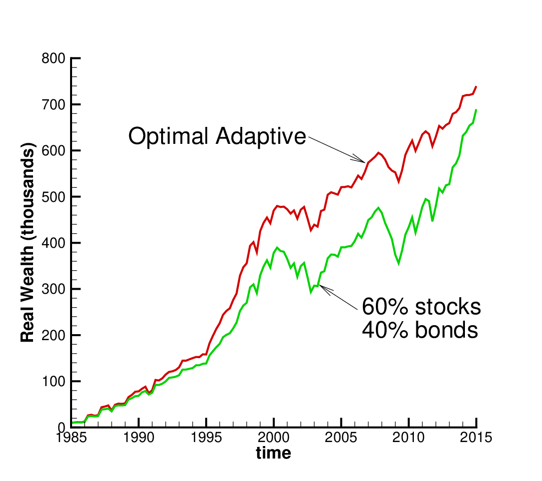
Figure 1(a) compares the adaptive strategy with a constant proportion strategy. We can see that both strategies ended up with roughly the same total real wealth, but the strategy had a very rough ride during the dot-com bubble (2002) and the financial crisis (2008).
Alternatively, Figure 1(b) compares the adaptive strategy with the linear glide path. As advertised, the glide path strategy is much smoother than the strategy, but it ends up with considerably smaller (i.e. about 30% lower) real wealth in 2015 compared to the optimal adaptive strategy.
The optimal adaptive strategy appears to offer some advantages over both the constant proportion and the glide path strategies. Perhaps you are intrigued. How does this strategy work? We’ll see in the next Section.

3 Three possible solutions
Many studies have shown that individual investors generally do a poor job of investing. They tend to buy at market peaks, sell at bottoms, and are not well-diversified (Barber and Odean, 2013, see, e.g.). Target Date Funds (TDFs) (also known as Lifecycle Funds) are an attempt by the investment industry to provide a solution for retail clients, specifically those enrolled in a DC plan.11 1 According to Morningstar, there was over USD 750 billion invested in TDFs in the US at the end of 2015. The most basic TDF has only two possible investments: a bond index and an equity index. Given a specified target date (which would be the anticipated retirement date of the plan member), we consider here three possible methods to specify the bond/stock allocation in the DC investment portfolio: deterministic glide path, constant proportion, and an adaptive strategy.
3.1 Deterministic glide path
In this case, the allocation of stocks and bonds is determined by a glide path. This is currently a popular method used by many TDFs. Denoting time by , a simple example of a glide path is
The logic behind this idea is that you should take on more risk when you are young (with many years to retirement) and then take on less risk when you are older, with less time to recover from market shocks. This seems quite sensible. The investment portfolio is typically rebalanced at quarterly or yearly intervals, so that the equity fraction is reset back to the glide path value . This idea is so attractive that TDFs are Qualified Default Investment Alternatives (QDIAs) in the US. If an employee has enrolled in an employer-managed DC plan, the assets may be placed in a QDIA as a default option, in the absence of any instructions from the employee.
It is important to note that the glide path in the age-based example above is only a function of time . We call this type of strategy a deterministic glide path, i.e. this strategy does not adapt to market conditions or the investment goals of the DC plan member.
3.2 Constant proportion
A much simpler method is a constant proportion policy, which is also a common asset allocation method. In this strategy, we rebalance to a constant equity fraction at all rebalancing times. Of course, a constant proportion allocation is a special case of a glide path, where .
3.3 Adaptive strategies
In deterministic glide paths, rebalancing strategies are only a function of time. Let’s consider a strategy which allows the fraction invested in the risky asset to be a function of both time and accumulated wealth in the DC portfolio at , denoted by . Then , so that this an adaptive strategy.
We consider a target-based strategy, where we choose to minimize
| (3.1) |
where denotes terminal wealth at time , is target final wealth, and indicates expected (or mean) value. In other words, we seek the asset allocation strategy which minimizes the expected quadratic shortfall with respect to the target wealth .22 2 We assume that the initial wealth . Dang and Forsyth (2016) show that the optimal strategy has , so that . This means that only shortfall (not excess) is penalized in (3.1).
4 Comparing the three solutions
To provide a realistic comparison, we consider a plausible investment scenario and evaluate the three strategies under both (i) a parametric model which captures the broad statistical properties of the historical market, and (ii) bootstrap resamples of the historical market.
4.1 Investment scenario
We consider the prototypical DC investor example shown in Table 4.1. We assume that the investor makes an initial investment in the portfolio of $10,000 at time zero (i.e. ), and that she contributes $10,000 per year (measured in real terms, i.e. inflation-adjusted) to the DC fund. The investment horizon considered is years, with the last investment of $10,000 (real) being made at years.
| Investment horizon | 30 years |
| Synthetic market parameters | Historical data (1926:1-2015:12) |
| Initial investment | $10,000 |
| Real investment each year | $10,000 |
| Rebalancing interval | 1 year |
4.2 Estimating a parametric model for real equity returns
We construct two real indexes: a real total return equity index and a real short term bond index. Our data was obtained from the Center for Research in Security Prices (CRSP) through Wharton Research Data Services.33 3 More specifically, results presented here were calculated based on data from Historical Indexes, ©2015 Center for Research in Security Prices (CRSP), The University of Chicago Booth School of Business. Wharton Research Data Services was used in preparing this article. This service and the data available thereon constitute valuable intellectual property and trade secrets of WRDS and/or its third-party suppliers. We use the CRSP value-weighted total return index (“vwretd”), which includes all distributions for all domestic stocks trading on major US exchanges. We also use the 30-day Treasury bill return index from CRSP. Both this index and the equity index are in nominal terms, so we adjust them for inflation by using the US CPI index (also supplied by CRSP). We use real indexes since long term retirement saving should be trying to achieve real (not nominal) wealth goals.
Figure 1(a) shows a histogram of the monthly returns from the real total return equity index, scaled to unit standard deviation and zero mean. We superimpose a standard normal (Gaussian) density onto this histogram. The plot shows that the empirical data has a higher peak and fatter tails than a normal distribution, consistent with previous empirical findings for virtually all financial time series.
The fat left tails of the historical density function can be attributed to large downward equity price movements which are not well modelled assuming normally distributed returns. From a long term investment perspective, it is advisable to take into account these sudden downward price movements.
We fit the data over the entire historical period using a jump diffusion model (Kou and Wang, 2004). This provides a more accurate fit to the data, as illustrated in Figure 1(a). To show the fat left tail of the jump diffusion model, we have zoomed in on a portion of the fitted distributions in Figure 1(b).


4.3 Comparisons under the estimated model
We now compare the constant proportion, (optimal) deterministic glide path and optimal adaptive strategies under the estimated jump diffusion model with parameters estimated from the entire 1926:1 - 2015:12 data set (subsequently referred to as the synthetic market). Note that the jump diffusion model is applied only to the equity returns. Bond returns are simply determined from the sample average monthly change in the real bond index. We will use this synthetic market to determine optimal strategies and carry out Monte Carlo simulations.
In the following comparison, we consider a equity-bond split as the constant proportion strategy. In other words, at each annual rebalancing date we rebalance so that 60% of the portfolio is invested in equities and 40% in bonds. This is a special case of a glide path strategy, with for all times . The equity fractions at rebalancing times for the other two strategies are determined as follows:
- •
Deterministic glide path strategy: we calculate the equity fraction at each rebalancing date such that the standard deviation of terminal wealth is as small as possible under the restriction that the expected value of terminal wealth matches the corresponding expected value for the constant proportion strategy.
- •
Adaptive strategy: we calculate the equity fraction at each rebalancing date such that the mean quadratic target error is as small as possible with the target set so that the expected value of terminal wealth is the same as for the constant proportion strategy.
We determine the optimal rebalancing fractions by using a computational optimization method (glide path) and solving a Hamilton Jacobi Bellman equation (adaptive strategy). In each case, we constrained the equity fraction so that (no shorting and no leverage).
Figure 2(a) shows the optimal deterministic glide path. Figure 2(b) displays the mean fraction invested in equities for the adaptive strategy, and its standard deviation.44 4 Since the adaptive strategy depends on the accumulated wealth so far, it is non-deterministic. As a result, we plot both the mean and the standard deviation of the equity fraction. On average, the adaptive strategy maintains a high allocation to stocks for longer than the deterministic strategy, but de-risks faster as we approach retirement. The constraint is clearly active for both strategies at early times.


Table 4.2 compares the results for the constant proportion ), optimal deterministic glide path, and adaptive strategies. All three strategies by design deliver the same expected value. The optimal deterministic standard deviation is about of the constant proportion strategy, a very small improvement. The standard deviations of the glide path and constant proportion are more than twice as large as that of the adaptive strategy. Table 4.2 also shows some information about shortfall probabilities. For example, the probability of achieving a final real wealth less than $650,000 is about 43% for both the constant proportion the and optimal deterministic strategies. For the adaptive strategy, the probability of achieving a final wealth less than $650,000 is only 22%.
Based on these synthetic market results for this case with regular contributions, it is possible to come up with a deterministic glide path which beats a constant proportion strategy, but not by very much. The adaptive strategy, on the other hand, significantly outperforms both the optimal deterministic glide path and the constant proportion strategies. We have repeated these tests with many different synthetic market parameters. As long as the investment horizon is longer than 20 years, the differences in performance between the optimal deterministic glide path and the constant proportion strategy with equivalent terminal wealth are very small, and each of these are clearly dominated by the adaptive strategy.
| Probability of Shortfall | |||||
|---|---|---|---|---|---|
| Strategy | |||||
| Constant proportion | $824,000 | $512,000 | .23 | .44 | .60 |
| Deterministic glide path | $824,000 | $503,000 | .23 | .43 | .60 |
| Optimal adaptive | $824,000 | $242,000 | .15 | .22 | .31 |
4.4 Comparisons under bootstrap resampling
The synthetic market results are based on fitting the historical returns to a jump diffusion model. This model assumes that monthly equity returns are statistically independent, which is debatable. In order to get around artifacts introduced by our modelling assumptions, we test the three strategies using a bootstrap resampling method. This can be viewed as a more realistic test, in the sense that we can observe how the strategies would have performed on actual historical data.
Our investment horizon is years. Each bootstrap path is determined by dividing into blocks of size years, so that . We then select blocks at random (with replacement) from the historical data set. Each block starts at a random month. We then concatenate these blocks to form a single path. We repeat this procedure times and generate statistics based on this resampling method.
The idea here is that if the real data shows some serial dependence, then this will show up in the bootstrap resampling. Based on some econometric criteria, we use a blocksize of years. We have experimented with blocksizes ranging from years, and the results are qualitatively similar. Note that the rebalancing strategies continue to be determined from the synthetic market as described above. We emphasize that the resampled paths are applied to both the equity index and the bond index. In addition to serial dependence, we are also introducing random variations in the bond component through the resampling.
The bootstrap results are shown in Table 4.3. Of course, now that we use the actual historical returns (with a random starting point), the mean terminal wealth for the adaptive strategy is no longer equal to the mean terminal wealth for the constant proportion strategy. This reflects the fact that our strategies were computed based on the jump diffusion model with constant interest rates, which is obviously an imperfect representation of reality. Nevertheless, as for the synthetic market tests, the adaptive strategy significantly dominates both the constant proportion and the deterministic glide path strategies.
We emphasize that the adaptive strategy was based only on the the long term average parameters obtained by fitting a jump diffusion model to the entire historical data set. This same strategy was then used for all the simulated bootstrap resampled paths. No tuning of the strategy for any particular path was used.
| Probability of Shortfall | |||||
|---|---|---|---|---|---|
| Strategy | |||||
| Constant proportion | $784,000 | $390,000 | .23 | .44 | .61 |
| Deterministic glide path | $784,000 | $382,000 | .22 | .43 | .62 |
| Optimal adaptive | $814,000 | $229,000 | .14 | .21 | .33 |
4.5 More on the optimal adaptive strategy
The target for the adaptive strategy was selected so that expected terminal wealth in the synthetic market matched that achieved by the constant proportion strategy. In practice, how should we pick ? A reasonable approach is to enforce the constraint
| (4.1) |
The investment goal in the case of retirement saving would be the amount required to fund a reasonable replacement level of income for a retiree. Of course in general, , i.e. in order to have wealth on average, we have to aim at a higher target.
It is also interesting to note that the adaptive strategy turns out to be dynamically mean variance optimal (Li and Ng, 2000; Dang and Forsyth, 2016). This means that for a specified mean terminal wealth , no other strategy has smaller variance. In addition, the adaptive strategy offers the opportunity in some cases to withdraw cash without compromising the probability of reaching the target (Dang and Forsyth, 2016; Forsyth and Vetzal, 2016).
5 Conclusion: Do target date funds need to adapt?
Of course, we have looked at only one possible adaptive strategy. There are many other possibilities. We argue that the adaptive strategy we have considered is especially appealing because it simultaneously minimizes two measures of risk: quadratic shortfall and variance (standard deviation).
However, our main point here is that restricting attention to deterministic glide paths is suboptimal. Investors can do a lot better by considering adaptive strategies. It is worthwhile to note that the vast majority of target date funds use deterministic strategies. Do target date funds need to adapt? The answer is clear: you need to adapt to your target.
References
- Barber and Odean (2013) Barber, B. M. and T. Odean (2013). The behavior of individual investors. In G. Constantinides, M. Harris, and R. Stulz (Eds.), Handbook of Economics and Finance, Chapter 22, pp. 1533–1569. Elsevier.
- Dang and Forsyth (2016) Dang, D.-M. and P. Forsyth (2016). Better than pre-commitment mean-variance portfolio allocation strategies: a semi-self-financing Hamilton-Jacobi-Bellman equation approach. European Journal of Operational Research 250, 827–841.
- Forsyth and Vetzal (2016) Forsyth, P. and K. Vetzal (2016). Robust asset allocation for long-term target-based investing. submitted to the International Journal of Theoretical and Applied Finance, working paper, University of Waterloo.
- Graham (2003) Graham, B. (2003). The Intelligent Investor. New York: HarperCollins. Revised edition, forward by J. Zweig.
- Kou and Wang (2004) Kou, S. and H. Wang (2004). Option pricing under a double exponential jump diffusion model. Management Science 50, 1178–1192.
- Li and Ng (2000) Li, D. and W.-L. Ng (2000). Optimal dynamic portfolio selection: Multiperiod mean-variance formulation. Mathematical Finance 10, 387–406.