The Coulomb flux tube on the lattice
Abstract
In Coulomb gauge a longitudinal electric field is generated instantaneously with the creation of a static quark-antiquark pair. The field due to the quarks is a sum of two contributions, one from the quark and one from the antiquark, and there is no obvious reason that this sum should fall off exponentially with distance from the sources. We show here, however, from numerical simulations in pure SU(2) lattice gauge theory, that the color Coulomb electric field does in fact fall off exponentially with transverse distance away from a line joining static quark-antiquark sources, indicating the existence of a color Coulomb flux tube, and the absence of long-range Coulomb dipole fields.
Keywords:
Confinement,lattice gauge theoriespacs
11.15.Ha, 12.38.AwI Introduction
Coulomb gauge has been used in many studies of quark confinement, beginning with the seminal work of Gribov [1], later elaborated by Zwanziger [2]. In this gauge the color Coulomb potential (defined below) is confining, and there is some hope that this confining behaviour can be derived or understood analytically, e.g. by Schwinger-Dyson equations, variational methods, or some other approach. A sample of work along these lines is found in [3, 4, 5, 6, 7, 8, 9]. Coulomb gauge also has the advantage that physical states are obtained by operating on the vacuum with local field operators. This allows us to define what is meant by “constituent” gluons in hadronic states, and to construct e.g. glueball states by operating on the vacuum with -field operators in the appropriate combinations of spin and parity.
The color Coulomb potential is the interaction energy of the state generated by quark-antiquark creation operators acting on the ground state, i.e.
| (1) | |||||
where is the Coulomb gauge Hamiltonian and is an -independent constant. We will consider static quarks in the infinite mass limit, with the quark located at position , the antiquark at position ,and the state is
| (2) | |||||
where is the ground state, are quark and antiquark creation operators, is a color index, is a normalization constant, and the polarizations are unimportant in what follows. For convenience we take to be the origin, and to lie along the -axis. It is well known from lattice simulations [10, 11, 12, 13, 14, 15] that is a linearly confining potential. What has not been investigated up to now is the spatial distribution of the color Coulomb field which gives rise to this potential.
The reason that there is any -dependence at all in the energy expectation value is due to the fact that, in Coulomb gauge, the creation of charged sources is always accompanied, because of the Gauss law constraint, with an associated longitudinal electric field. To briefly review this point: In Coulomb gauge the dynamical degrees of freedom are the transverse fields. Separating the color electric field into a transverse and longitudinal part, where , the Gauss law constraint becomes
| (3) |
where is the covariant derivative, and
| (4) |
are the color charge densities due to the quark and gauge fields, respectively, with the generators of the Lie algebra, and the structure constants. Let
| (5) |
be the inverse of the Faddeev-Popov operator. Then the longitudinal electric field is determined to be
| (6) |
We are interested in the part of which is generated by the quark-antiquark sources, namely
| (7) |
Now suppose is a typical vacuum fluctuation, where the word “typical” is best defined with a lattice regularization: these are thermalized configurations generated by the lattice Monte Carlo procedure, transformed to Coulomb gauge. Squaring , summing over the color index , and taking the expectation value of the matter field color charge densities in the massive quark-antiquark state, a straightforward calculation leads to the matter contribution
| (8) | |||||
where is the number of colors. It seems unlikely that would fall exponentially with for typical vacuum configurations. In that case it is hard to see how the color Coulomb potential, which depends on the interaction kernel
| (9) |
could rise linearly at large . Moreover, the expectation value of the Fourier transform of , which is the momentum-space ghost propagator , has been computed in lattice Monte Carlo simulations, both in SU(2) [16, 14, 17] and SU(3) [18] pure gauge theory, with the result
| (10) |
in the infrared, corresponding to an asymptotic behavior in position space. So it is reasonable to assume some power-law falloff of with separation , for typical vacuum fluctuations . Then, unless there are very delicate cancellations among the terms in (8), one would expect a power law falloff for , as the distance of point from the sources increases. This would imply a long-range color Coulomb dipole field in the physical state .
It should be emphasized that is not the minimal energy state containing a static quark-antiquark pair. For that reason is clearly an upper bound on the potential of a static quark-antiquark pair, and if the static quark-antiquark potential is confining, then so is the color Coulomb potential (a point first made in [19]). In fact, lattice simulations [12, 13] show that the color Coulomb potential in SU(3) pure gauge theory is about a factor of four greater than the usual asymptotic string tension. If one would begin with the physical state (2) and let it evolve in Euclidean time, then the state will evolve to the minimal energy state with potential , and the initial color Coulomb electric field will evolve into the standard flux tube configuration. It has been suggested [20] that in Coulomb gauge the minimal energy flux tube state is best understood in the framework of the gluon chain model [21], where we consider more general states of the form
| (11) | |||||
and the order of color indices of the fields is correlated with position in the chain. In principle such states can reduce the Coulomb string tension to the asymptotic string tension; the details can be found in [13, 20]. In this article, however, we will be concerned with the distribution of the Coulomb electric field associated with the state , and the question we address here is whether this color dipole gives rise to a long range Coulomb field, or whether instead the Coulomb electric field is somehow collimated from the moment of creation of the static quark-antiquark pair, even before that field has a chance to evolve into a minimal energy flux tube.
II Lattice Setup
We work in the framework of the Euclidean path integral of SU(2) lattice gauge theory in Coulomb gauge
| (12) |
where is the Faddeev-Popov determinant in Coulomb gauge, and in this article we will neglect the issue of Gribov copies. To compute the Coulomb potential, let
| (13) |
Then the Coulomb energy is obtained from the logarithmic time derivative [10, 11]
| (14) |
while the minimal energy of static quark-antiquark state is obtained in the opposite limit
| (15) |
Now in Coulomb gauge the correlator has an instantaneous part
| (16) | |||||
where is the non-instantaneous part. It was shown by Zwanziger [2, 22] that both and are renormalization group invariant. Expanding in a power series and extracting the -dependent part of , it is clear that
| (17) |
where is the quadratic Casimir of the fundamental representation.
The lattice version of (14) in SU() pure gauge theory is the logarithm of the equal times timelike link correlator
| (18) |
where is in lattice units, and in this form has been computed in numerical simulations. Dividing by the lattice spacing to convert to physical units, it was found that
| (19) |
where is the lattice spacing and . In physical units the Coulomb string tension , and the dimensionless constants , appear to have finite non-zero limits as , with the Coulomb string tension approximately four times larger than the asymptotic string tension, as shown in the SU(3) Coulomb gauge lattice simulations of ref. [13]. An intriguing fact is that appears to go to in the continuum limit, which is the Lüscher value expected for the QCD flux tube. That could be a numerical coincidence, although this value of is also roughly consistent with a best fit of our on-axis data for at , shown in Fig. 1. If this proximity to is not a coincidence, and does indeed have a string origin of some kind, that would be interesting to know. This is part of our motivation to study the spatial distribution of the Coulomb electric field due to static quark-antiquark charges.

For our purposes it is sufficient to study how the color electric field depends on the transverse distance away from the midpoint of a line joining the quark and antiquark. Let the quark and antiquark lie along the -axis, say, with and unit vectors in the directions, and define
| (20) |
The quantity we wish to compute is the contribution to the -component due to the quark-antiquark pair, i.e.
| (21) |

The lattice version of (21) is , where
| (22) |
and where
| (23) |
is a plaquette operator, with
| (24) |
and the expectation values are evaluated in Coulomb gauge. The lattice operator in the numerator of (22) is illustrated in Fig. 2. Of course there is nothing special about the -directions or the time-slice, so in practice we average over observables which differ only by spacetime translations and 90∘ spatial rotations (Coulomb gauge precludes changing the orientation in time).



III Results
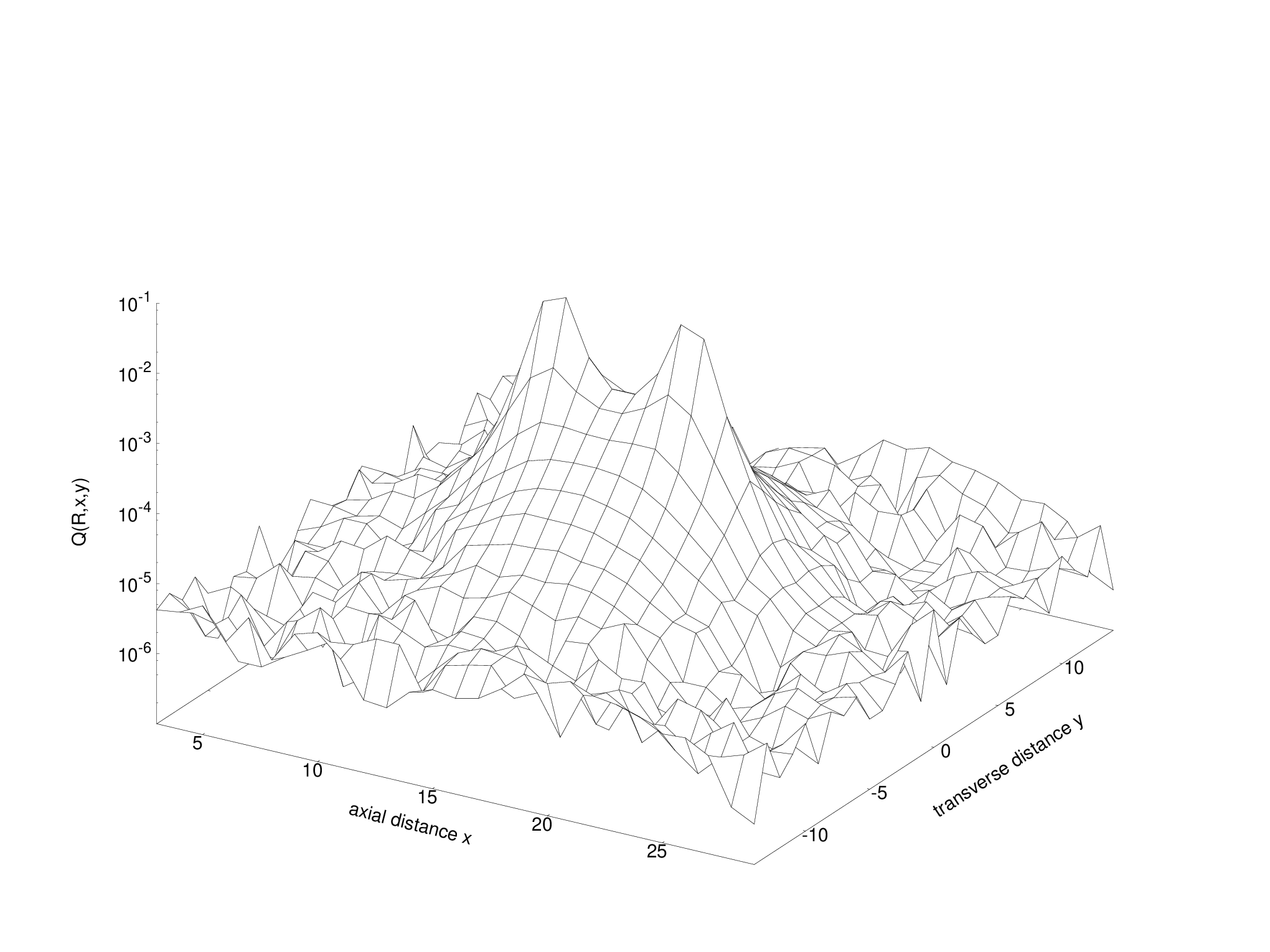
Our results for quark-antiquark separations , and transverse separations , obtained from lattice Monte Carlo simulation of pure SU(2) gauge theory at on a lattice volume, are shown in the logarithmic plots of Fig. 3. This data seems to rule out, fairly conclusively, any mild power-law falloff of the color electric energy density with transverse distance from the midpoint. The falloff with at fixed instead seems to be very nearly a pure exponential, at least until the error bars are comparable to the values of the data points. The Coulomb electric field of the quark-antiquark dipole is therefore not long range, but rather is collimated along the axis of the quark-antiquark pair. In other words, we appear to be seeing a Coulomb flux tube. Comparison of Fig. 3(g) to a plot of the center plane action density in the asymptotic (or minimal energy) flux tube, shown in Fig. 14 of ref. [23], indicates that the Coulomb flux tube is substantially narrower than the minimal energy flux tube, with a width smaller by about a factor of 1.7.11 1 Figure 14 in ref. [23] was also taken at , for a quark-antiquark separation of 8 lattice spacings. This is an indication that the finite width of the Coulomb flux tube cannot simply be attributed to the finite size of (in ) equal to the lattice spacing, in the lattice version (18) of the correllator (14). If it were the case that the width was infinite at (i.e. power law falloff), and shrunk to the width of the minimal energy flux tube at , then we would expect the width of the flux tube at finite lattice spacing to be greater than the width of the minimal energy flux tube, whereas the reverse is what we actually find.
Profiles of the flux tube (or, more precisely, the component ) at a quark-antiquark separation of are shown in Fig. 4. In this case we are computing an observable defined by the right hand side of (22), but with point defined by
| (25) |
Note the logarithmic scale on the vertical axis of Fig. 4 . On a linear scale, the values in the transverse direction are soon indistinguishable from zero.
A natural question is whether the exponential falloff in the transverse direction is directly related to the exponential falloff of the timelike link correlator, from which we have extracted the color Coulomb potential. For example, we might ask whether the connected correlator of the timelike links and timelike plaquette can be viewed as a four timelike link correlator, which factorizes into a product of two point functions. Coulomb gauge brings spatial links as close as possible to the identity, so if we approximate
| (26) |
then the numerator in (22) involves a four-point equal-time correlator of timelike links. Let us suppose that the connected part approximately factorizes into a product of two-point functions
In that case we would expect
| (28) |
where is a constant. In fact this is not even close to a fit of the data, as seen in Fig. 5 for . The exponential falloff of the Coulomb flux tube in the transverse direction is much faster than , and this two-point correlator description simply fails to give a reasonable account of the data.

Returning to the expression (8), and the observed power law behavior of the ghost propagator (10), there is the question of how the Coulomb energy density could fail to also have a power law falloff. The only possibility we see is that the “typical” vacuum configurations which account for the expectation value of the ghost propagator are not the dominant configurations in the expectation value of products of the operators, such as . The expectation value of the product must be very sensitive to exceptional field configurations, possibly ones in which the lowest eigenvalue of the Faddeev-Popov operator is unusually small, which do not greatly affect the expectation value of the operator by itself. Presumably these exceptional configurations, for reasons that are not clear to us, must be responsible for the rather precise cancellations among the different terms in (8) that are required for an exponential falloff.
IV Conclusions
Confinement in Coulomb gauge seems to be more subtle than simply a linear potential from dressed one-gluon exchange, i.e. . While this two point function is no doubt part of the story, it is not the whole story, since the two point function, although linearly rising, is not by itself an explanation for the formation of a Coulomb electric flux tube. One may speculate that the Coulomb string tension derives from the same underlying mechanism (center vortices come to mind) that accounts for the asymptotic string tension. In particular, the confining two point function is thought be due to a non-perturbative enhancement in the density of near-zero eigenvalues of the Faddeev-Popov operator, associated with the proximity of typical vacuum configurations to the Gribov horizon. It has been shown via lattice Monte Carlo simulations that removal of center vortices from thermalized lattice configurations sends this eigenvalue density back to the perturbative form [24], and the corresponding Coulomb string tension (along with the asymptotic string tension) vanishes upon vortex removal [10] (for recent developments in the vortex picture, see [25, *Kamleh:2017lij]). If center vortices or some other topological objects are responsible for the linearly rising Coulomb potential, it is probably necessary to also appeal to a topological mechanism in order to understand the formation of a Coulomb flux tube.
Acknowledgements.
This research is supported by the U.S. Department of Energy under Grant No. DE-SC0013682.References
- [1] V. N. Gribov, Nucl. Phys. B139, 1 (1978).
- [2] D. Zwanziger, Nucl. Phys. B518, 237 (1998).
- [3] A. P. Szczepaniak and E. S. Swanson, Phys.Rev. D65, 025012 (2002), arXiv:hep-ph/0107078.
- [4] A. P. Szczepaniak, Phys.Rev. D69, 074031 (2004), arXiv:hep-ph/0306030.
- [5] C. Feuchter and H. Reinhardt, Phys.Rev. D70, 105021 (2004), arXiv:hep-th/0408236.
- [6] D. Epple, H. Reinhardt, and W. Schleifenbaum, Phys.Rev. D75, 045011 (2007), arXiv:hep-th/0612241.
- [7] D. Zwanziger, Phys. Rev. D70, 094034 (2004), arXiv:hep-ph/0312254.
- [8] R. Alkofer, A. Maas, and D. Zwanziger, Few Body Syst. 47, 73 (2010), arXiv:0905.4594.
- [9] M. Golterman, J. Greensite, S. Peris, and A. P. Szczepaniak, Phys. Rev. D85, 085016 (2012), arXiv:1201.4590.
- [10] J. Greensite and S. Olejnik, Phys.Rev. D67, 094503 (2003), arXiv:hep-lat/0302018.
- [11] J. Greensite, S. Olejnik, and D. Zwanziger, Phys.Rev. D69, 074506 (2004), arXiv:hep-lat/0401003.
- [12] Y. Nakagawa, A. Nakamura, T. Saito, H. Toki, and D. Zwanziger, Phys.Rev. D73, 094504 (2006), arXiv:hep-lat/0603010.
- [13] J. Greensite and A. P. Szczepaniak, Phys.Rev. D91, 034503 (2015), arXiv:1410.3525.
- [14] G. Burgio, M. Quandt, and H. Reinhardt, Phys.Rev. D86, 045029 (2012), arXiv:1205.5674.
- [15] A. Voigt, E.-M. Ilgenfritz, M. Muller-Preussker, and A. Sternbeck, Phys.Rev. D78, 014501 (2008), arXiv:0803.2307.
- [16] G. Burgio, M. Quandt, and H. Reinhardt, Phys.Rev.Lett. 102, 032002 (2009), arXiv:0807.3291.
- [17] K. Langfeld and L. Moyaerts, Phys. Rev. D70, 074507 (2004), arXiv:hep-lat/0406024.
- [18] Y. Nakagawa et al., Phys.Rev. D79, 114504 (2009), arXiv:0902.4321.
- [19] D. Zwanziger, Phys.Rev.Lett. 90, 102001 (2003), arXiv:hep-lat/0209105.
- [20] J. Greensite and A. P. Szczepaniak, Phys. Rev. D93, 074506 (2016), arXiv:1505.05104.
- [21] J. Greensite and C. B. Thorn, JHEP 0202, 014 (2002), arXiv:hep-ph/0112326.
- [22] A. Cucchieri and D. Zwanziger, Phys.Rev. D65, 014002 (2001), arXiv:hep-th/0008248.
- [23] G. S. Bali, K. Schilling, and C. Schlichter, Phys. Rev. D51, 5165 (1995), arXiv:hep-lat/9409005.
- [24] J. Greensite, S. Olejnik, and D. Zwanziger, JHEP 05, 070 (2005), arXiv:hep-lat/0407032.
- [25] D. Trewartha, W. Kamleh, and D. Leinweber, Phys. Lett. B747, 373 (2015), arXiv:1502.06753.
- [26] W. Kamleh, D. B. Leinweber, and D. Trewartha, in Proceedings, Lattice 2016, arXiv:1701.03241.