Estimating Thresholding Levels for Random Fields via Euler Characteristics
We introduce Lipschitz-Killing curvature (LKC) regression, a new method to produce thresholds for signal detection in random fields that does not require knowledge of the spatial correlation structure. The idea is to fit observed empirical Euler characteristics to the Gaussian kinematic formula via generalized least squares, which quickly and easily provides statistical estimates of the LKCs — complex topological quantities that can be extremely challenging to compute, both theoretically and numerically. With these estimates, we can then make use of a powerful parametric approximation via Euler characteristics for Gaussian random fields to generate accurate thresholds and -values. The main features of our proposed LKC regression method are easy implementation, conceptual simplicity, and facilitated diagnostics, which we demonstrate in a variety of simulations and applications.
and
Technion, Renaissance Technologies, Harvard and Columbia.
??Research supported in part by US-Israel Binational Science Foundation, 2008262.??Research supported in part by FP7-ICT-318493-STREP.??Research supported in part by ERC 2012 Advanced Grant 20120216.??Research supported in part by NIH/NIGMS,R01GM090202 and NSF, DMS-1510446.AMS 2000 subject classifications: Primary 60G60, 62G32, 62E20 ; Secondary 60G15, 62M30, 62M40.
Keywords and phrases:
Brain imaging, Gaussian kinematic formula, Lipschitz-Killing curvature, design points, excursion set, regression, significance level, covariance.
1 Introduction
1.1 Pre-History
The paper that you are (maybe) about to read was started in 2008, when RJA spend a semester at Harvard and talked a lot with SCK. During a lecture, RJA made the claim that estimating Lipschitz-Killing curvatures (defined below) was a hard problem, at which stage SCK commented “It doesn’t seem all that hard. Why can’t you just treat it as a regression problem?” At the time KB was a graduate student, listening to the same lecture, and all three got together to write the first version of this paper. Since RJA returned to the Technion, and KB graduated and moved to Renaissance Technologies, it took until 2011 for a final first version to be submitted for publication. A few months later it was rejected (from an excellent journal) but, since the authors still liked their paper they set about preparing a revision, this time together with AM, who was then a postdoctoral fellow at the Technion. In 2014 the new version was submitted to a different (and even better) journal, only to be rejected since it was too methodological and not applied enough, but with some nice ideas for rewriting as long as the authors were prepared to rewrite everything in such a way that it made the referees happy and them miserable.
Now that AM has left the Technion and is doing other things, RJA is (happily) approaching retirement, KB is well entrenched in industry, and AM is also busy with new problems, it seems unlikely that this paper will ever get revised again. But, the four authors still like it, and it keeps getting cited (seemingly implying that others share their opinion) and so the time has come to put what there is up on arXiv. Which is why what you are reading is a 2017 arXiv deposit of what is basically a 2011 paper.
1.2 Motivation
Random field models are widely used in many scientific applications, including the description of spatial structures in environmental and epidemiological studies, the statistical analysis of brain images, and the modeling of the cosmic microwave background radiation, as well as other cosmological phenomena. An important problem of interest common to most of these applications is the determination of threshold levels for the random field, which indicate that regions with values above the level are, in some sense, significant, while regions with values below are not. Accurate determination of threshold levels for random fields faces a major challenge that the simpler setting of independent observations does not: the values of random fields are correlated in space.
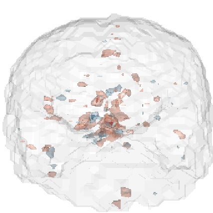
A concrete example that we will study in this paper is an experiment involving functional magnetic resonance imaging (fMRI), which was a language priming experiment carried out by Dehaene-Lambertz et al. (2006) that appeared in the functional image analysis contest (FIAC). fMRI responses were measured twice for 16 subjects after each heard a sentence spoken under two different conditions: once with the same speaker both times, and once with different speakers. After each repetition, hemodynamic activity was measured at every point (voxel) in a 64 64 30 grid that encompasses the brain for each subject. The fMRI scan for the first subject is shown in Figure 1.1: the light and dark red domains represent mid- and high-activation regions of the brain, respectively, under the same-speaker (upper left) and different-speaker conditions (lower left).
| Subject 1 | Subject 1 | Subject 1 |
| Same-speaker | Difference | Studentized Residual |
 |
 |
 |
| Subject 1 | All Subjects | All Subjects |
| Different-speaker | Average Difference | Statistic |
 |
 |
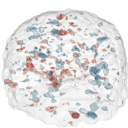 |
This study inspires two important research questions: Firstly, are there any significant differences at all? Secondly, if there are, where do these significant differences lie? A natural way to look for differences is to compare the two conditions at every voxel in the brain. Figure 1.1 (lower right) shows the result of voxelwise paired tests: in red regions, different-speaker activity exceeds same-speaker activity; in blue regions, the opposite is true. The light and dark colored regions show areas where the statistics exceed the nominal single-test 95% and 99% levels of 2.13 and 2.95, respectively. The multiplicity of comparisons of 24,759 voxels in the brain, each with its own test, poses a challenge in establishing significance. Using the 95% threshold, 1,273 voxels indicate significant differences, which, as a proportion of 24,759, amounts to approximately 5%, and therefore mainly false positives. In contrast to these excessive false positives using the test 95% threshold, using the 95% Bonferroni bound of 7.23 indicates there are no significant differences at all. This bound is known to be very conservative, and the resulting conclusion of no significant results whatsoever is unconvincing, and moreover, unlikely to be inconsistent with neurological hypotheses. Furthermore, in considering the nature of fMRI studies, the strength of spatial dependence depends on the resolution, among other factors, and should thus also be taken into consideration. These preliminary exploratory results underline the importance of our motivating research questions and provide the impetus for a sound method to determine and characterize significance.
1.3 Tail probabilities and Euler characteristics
As a starting point, let the null hypothesis assert that both brain scans, under both conditions, are, on average, equivalent. For the moment, assume that rather than having voxel-based data, we observe the fMRI images over a continuum. Issues of resolution and discretization will be addressed and formalized later. Under such an , the grid of -statistics is a smooth random field over a region of the brain. Since high values of usually indicate deviation from , a natural test statistic to consider is then the maximum
The problem with using as a test statistic, however, is that its null distribution is required, but is virtually never known. In the FIAC data, = 6.08; a test of requires the -value, . In addition, to identify the activated regions of , we require a 5% threshold such that = 0.05. Obtaining these unknown quantities, the null distribution and the threshold, is difficult because they both depend on the correlation structure of , which itself is also unknown.
To bypass this problem, we make use of a powerful parametric method for determining the null tail probabilities of for a wide class of Gaussian and Gaussian-related random fields: the Euler characteristic heuristic (ECH) (Adler, 2000), which provides an accurate approximation to the exceedence probability for large (i.e. high levels or thresholds ), where “large” refers to values of of the order of 5% or smaller, and “accurate” refers to an error in approximation of the order of 1% to 2% in the threshold level. (i.e. A true threshold of, say, 5, in standardised units, will be estimated by a value in the range (4.99,5.01).) The ECH has been widely used in topological inference in fMRI studies (Cao and Worsley, 1999; Friston et al., 1994; Kilner and Friston, 2010; Shafie et al., 2003; Worsley, 1994; Worsley, 1995a; Worsley, 1995b, e.g.,), cosmological data (Bardeen et al., 1986; Gott et al., 2008; Gott et al., 2007; Torres, 1994; Vogeley et al., 1994, e.g.,), as well as a number of other areas. Moreover, for smooth Gaussian random fields, the ECH is not merely a heuristic: it is a rigorous theory (Taylor, Takemura and Adler, 2005; Adler and Taylor, 2007).
The ECH is based on the Euler characteristic (EC) , an important topological quantity for many general classes of well-behaved sets. For a 3-dimensional Euclidean volume , counts the number of each of the three types of topological features of a manifold — (i) solid, simply connected regions of the manifold, or connected components, (ii) visible, open holes or handles, and (iii) invisible, closed holes or voids — in an alternating sum. It is a topological invariant, i.e. a property of a topological space that is invariant under homeomorphisms, or continuous deformations, of the topological space. It is given by
| # connected components in | (1.1) | ||||
The ECH considers the ECs of a specific case, that of the excursion sets ,
| (1.2) |
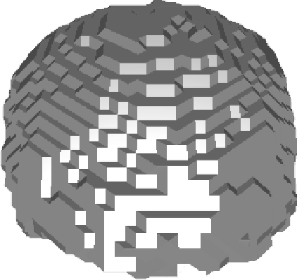
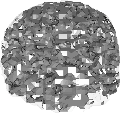
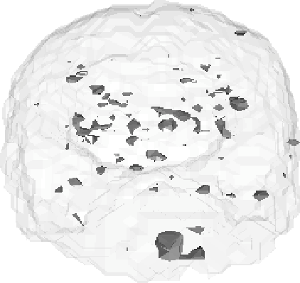
Figure 1.2 shows examples of and for varying ; is an integer that can be negative (middle left), positive (middle right) or close to zero (rightmost). Since topological features of the manifold lying below the level are effectively ignored, the manifold (and thus also the EC) becomes simpler as moves higher: At moderately high levels of , typically takes on the simplified form of a union of simply connected components, while at the highest levels, it either disappears completely (i.e. it is empty) or all that remains is a single simple component. Thus, at such high levels, the EC is either zero or one. Based on this phenomenon, the ECH claims that the expected EC for high approximates the tail probability,
| (1.3) |
A further result based on this phenomenon of topological simplification of excursion sets with increasing is that the expected EC is guaranteed to lie in for high enough. From (1.3), we obtain the required -value for , which can then be inverted to find the , or the threshold, corresponding to a confidence level, via the approximation
| (1.4) |
 |
 |
 |
 |
When considering random fields (Adler and Taylor, 2007, see) with constant mean and variance (which for the moment we take to be zero and one), the ECH provides the additional practicality of a parametric closed form for the expected EC , given by the Gaussian kinematic formula (GKF) (Taylor, 2006),
| (1.5) |
Here the are functions that usually take on a simple and explicit form. For example, if the random field is Gaussian, then the are explicitly expressible in terms of Hermite polynomials, as we shall see in (2.7) below. Other examples can be found in Adler (1981); Adler and Taylor (2011); Adler, Taylor and Worsley (2015?). The functions , which depend on both the domain and the covariance of , are the Lipschitz-Killing curvatures (LKCs), or intrinsic volumes, of — complex topological quantities that are often extremely difficult to evaluate theoretically, even for dedicated topologists, as well as numerically. When known, however, the LKCs provide the expected EC for all via the GKF (1.5), which can in turn be substituted into (1.3) provided by the ECH to obtain an approximate -value for or into (1.4) to obtain a threshold level. The estimation of the LKCs is the bottleneck of a successful application of the ECH and is the central concern of this paper.
1.4 Estimating Lipschitz-Killing curvatures
We introduce a new approach that estimates the LKCs by simply matching the expected and empirical ECs, which then directly yields the -value and threshold level in a straightforward manner via (1.3), (1.4), and (1.5). Figure 1.3 provides an illustration of our method: the left panel shows the empirical profiles for the 16 observed fields from the FIAC data (thin gray lines) and their sample average (solid black line) for different values of . We find the best-fitting LKCs through a generalized least squares regression of (1.5). The fitted LKCs then produce the best-fitting profile: the dashed black line. The intersection of this fitted profile and the 0.05 line yields the 95% confidence threshold as = 4.19 (black dot). This threshold can be applied to the brain of statistics to identify significantly activated regions. Doing this indicates only 7 voxels activated beyond 4.19 — a striking contrast to the 1,273 found using the naive -test 95% threshold of 2.13, and also more credible than the 0 found using the 95% Bonferroni bound of 7.23.


One caveat of which to take note in matching expected and empirical ECs is that the observed (empirical) ECs at very high levels of are generally too noisy to directly estimate the threshold ; calculating a threshold from extreme empirical ECs is akin to estimating a tail quantile with a small number of observations (16, for the FIAC data). The right panel of Figure 1.3 illustrates this phenomenon by zooming in and showing that the empirical and expected ECs cross the 0.05 line at very different values of . In cases of very high , for general -value approximation and threshold level determination, use of the expected EC yields significantly more reliable and accurate results that do not depend on small sample sizes, but instead derive from rigorous probability theory and topology.
Inference via LKC regression is parametric because it relies on the ECH, which leverages on an assumed underlying Gaussianity. A commonly suggested nonparametric alternative is a permutation test on the group assignments (same-speaker, different-speaker) to approximate the null distribution of . The main drawback of this nonparametric option is the tremendous expense of computing the maximum -statistic given a set of permuted labels, which is severely impeded by the computation of many hundred thousand voxelwise averages and standard deviations. For the FIAC data, a permutation test with just 100 permutation samples takes several hundred times longer than LKC regression. Moreover, observed random fields are typically Gaussian-related by construction, since they arise as the residual of some statistical procedure. Nonparametric methods generally underperform in cases where such distributional properties are known.
To date, the only other existing estimation method for LKCs is the warping method of Taylor and Worsley (2007). Warping transforms the realizations of the random field to a volume in a -dimensional space, where is the number of random fields in the data; for the FIAC data =16. The intrinsic volumes of the transformed volume are shown to be good estimates of the LKCs. Though accurate, understanding the method requires a knowledge of Riemannian geometry, and can be computationally slow, particularly for high dimensions. Compared to Taylor and Worsley (2007), our method has similar accuracy but is computationally faster. Furthermore, it requires only the ECs of the observed random fields. Since observations are typically taken over a regular grid, efficient numerical optimization is available. The warping method, on the other hand, must perform the slower computation of intrinsic volumes on a high-dimensional transformed space with irregularly spaced points.
1.5 Paper structure and acknowledgements
The remainder of this paper is organized as follows: In Section 2, we introduce our regression-based estimation method, detailing on the various implementation factors and combinations available, and their associated issues of optimality. Section 3 presents the results of a large scale simulation study, which compares these various factors and their combinations, as well as our approach to the warping method of Taylor and Worsley (2007). In Section 4 we extend this comparison from simulation studies to the concrete example of the FIAC data. Section 5 concludes the paper with a summary of its main results and proposals for other areas where our method would be applicable. The Appendix provides a brief treatment of the Gaussian kinematic formula (1.5).
Finally, we would like to thank Jonathan Taylor for helpful discussions at various stages of this work, and Naor Alush for help with the programming.
2 Lipschitz-Killing Curvature Regression
The goal of our regression method is to obtain accurate estimates of the Lipschitz-Killing curvatures (LKCs) for use in -value calculation and threshold level determination (see (1.2) and (1.4)). (While the LKCs are of interest in and of themselves, in this paper we shall concentrate almost exclusively on their importance for threshold determination.) The inputs are the observed realizations , , of a random field, assumed to be Gaussian or Gaussian-related and normalized to mean zero and unit variance, over a region .
The Gaussian kinematic formula (GKF) (1.5), combined with the central limit theorem, suggests a linear model with heteroscedastic, possibly correlated errors:
| (2.6) | |||||
for some unknown . The response variable is the average of the empirical Euler characteristics (ECs). The regressors take on a simple and explicit form; when the random field is Gaussian,
| (2.7) |
where is the -th Hermite polynomial. We estimate the unknown LKCs through generalized least squares (GLS).
Once the LKCs are estimated, we easily obtain an estimate of the expected EC via the GKF (1.5) for any level ,
which then substitutes into (1.3) to give an approximate -value for hypothesis testing for large , and into (1.4) to give a threshold level.
The validity of the GKF (1.5) for all forms the foundation of the effectiveness of our LKC regression method. For -value and threshold calculation, one typically encounters large values of , which correspond to small-probability events, the direct estimation of which is unreliable. Our regression approach, instead, is grounded on the observation that when is small or moderate, the expected EC can be well estimated from the data, since these cases do not correspond to small-probability events. These reliable estimates then translate, in turn, through our regression, into reliable estimates of the LKCs , which do not depend on ; the then yield good approximations for -values and threshold levels for large . In summary, LKC regression leverages the precision of estimation at low levels of to obtain accurate approximation at high levels of .
Several issues need to be addressed in the construction of our LKC regression method: First, to evaluate the empirical EC, the region for fixed must be determined, which poses a potential difficulty because each field is typically observed at a discrete grid of sample sites, yet, to apply the GKF, the excursion sets must be described as smooth regions over . We detail the construction of in Section 2.1. Second, compared to conventional linear regression, an interesting feature of our setting is that arbitrary amounts of “data” can be generated at very little cost, simply by exploiting (2.6) at a collection of specified levels . Each gives distinct excursion sets and their corresponding average EC,
However, this supposed advantage in fact raises the problem of a tradeoff between residual error in the regression and estimation error in the covariance matrix: additional data might help the regression, but the covariance matrix becomes increasingly difficult to estimate with more data. We address this tradeoff in detail in Section 2.3. Third, after specifying the levels , the unknown error covariance matrix must be estimated before running GLS. We present several estimation options in Section 2.2. In Section 3 we find optimal settings for level selection of and error covariance estimation.
As a tool for hypothesis testing, the LKC regression approach is powerful because it overcomes the need for the complete specification of the covariance structure of the random field. Very few assumptions about covariance are made; even isotropy is not required. The random fields only need be Gaussian or Gaussian-related, which is often a natural consequence of the data generating process.
2.1 Observed Excursion Sets
Though assumed to be continuous, in practice random fields are typically observed at a discrete set of sample sites . An empirical realization of a random field is thus defined by the observations ; Figure 2.4 provides an illustration. Sample sites commonly lie on a rectangular lattice for fields on the square and cube (upper left and middle) or on a latitudinal-longitudinal lattice for fields on the sphere (upper right). We measure the resolution of the field by the grid size , the number of sample sites in each direction/dimension; for example, for a 3D cube 20 corresponds to 8000.


In theory, to compute the EC of an excursion set , the excursion set needs to be represented as a smooth domain. However, as the fields are observed only at discrete points , an approximation of the exact domain is required. In the digital topology literature, there exist many constructions (Imiya and Eckhardt, 1999, e.g.,) of domains created from a set of points, known as quasi-objects. The methods are distinguished by their connectivity, which specifies how close two sample points must be for them to be considered part of the same domain. For example, in considering points on a planar lattice, 4-connectivity places vertically and horizontally adjacent points into the same domain, but diagonally adjacent points into separate domains (unless they also share an immediate neighbor); 8-connectivity includes all diagonal adjacencies in the same domain.
To create excursion sets from observed random fields, we use planar (2D) 8-connectivity and spatial (3D) 26-connectivity, where each point touches all its immediate and diagonal neighbors. This is equivalent to building by introducing a small square or cube centered at whenever , and then joining them to form the excursion set. For spherical fields, we use 8-connectivity over the latitudinal/longitudinal grid of sample sites, with the excursion sets made up of small plates. Figure 2.4 shows examples of the resulting excursion sets for fields on the plane (lower left), cube (lower middle) and sphere (lower right). We experimented with different connectivity structures, and concluded that they had little impact on the calculated ECs. In the brain image analysis example (FIAC, 64 64 30), we observed nearly identical EC profiles for spatial 6-connectivity, 18-connectivity, and 26-connectivity.
The final step in computing the response variable in the regression of (2.6) is to evaluate the EC for excursion sets. (1.1) provides a simple formula, provided we can count the number of connected components, handles, and voids. This calculation is easy in the discrete setting, in which the excursion set is made up of a large number of simple cells, such as squares, cubes or plates; the formula thus reduces to an alternating sum over distinct vertices, edges, faces and cubes of these cells:
| (2.8) |
The same formula also holds in two dimensions without the final term. A key advantage of our LKC regression method is the rapidity of this computation for cells on a grid; the warping method of Taylor and Worsley (2007), in contrast, must perform the slower computation of all intrinsic volumes (not just the EC) over an irregular (nonrectangular), warped grid.
For an application with realizations of the random field, LKC regression calls for the computation of ECs at different excursion levels. Taking advantage of binary search and careful indexing, the computation cost of our method is only . This makes it extremely fast to evaluate the EC for many levels .
2.2 Covariance of the Error Terms
The covariance structure of the error terms in LKC regression is defined by
We emphasize that should not be mistaken for the covariance of the random fields ; describes the correlation of the Euler characteristics across differing levels, and not of field values themselves. can be viewed as the covariance function of the stochastic process in .
The error covariance structure of LKC regression is nontrivial: First, they are heteroskedastic; the observed EC tends to be less variable at higher levels of , as illustrated in Figure 2.5 (upper right) for the FIAC data. Second, they are correlated; the sample correlation plot (lower left) and correlogram (lower right) show pronounced negative correlation for levels separated by about 1. This is due to the periodicity of the three swings in the EC profiles, which are about one (standardised) unit apart.


Given levels , LKC regression requires the covariance matrix . Although a misspecified covariance matrix still gives consistent estimates under GLS, the efficiency of the estimate depends on the estimation of . There are five ways of producing a positive-definite estimates of the covariance matrix :
- 1.
Identity (I). As a baseline, heteroskedasticity and correlation are ignored under this option so that , yielding an ordinary least squares (OLS) model.
- 2.
Smoothed diagonal (SD). Heteroskedasticity is incorporated while correlation is ignored. The sample variances are computed and then smoothed as a function of ; we employ local quadratic smoothing with 10% nearest neighbors (Loader, 1999; Loader, 2010). To prevent the smoothing procedure from generating negative variances, the smoothing is applied to the logarithm of the sample variances; values of with a sample variance of zero are dropped from the smoothing procedure. Examples of original and smoothed variances are depicted in Figure 2.6 (left panel). The covariance matrix is , where denotes the vector of smoothed variances.
- 3.
Smoothed correlogram (SC). This option uses the same smoothed variances of SD but assumes that the correlation between and is stationary, i.e. a function of the separation . Following a procedure in Hall, Fisher and Hoffman (1994), the sample correlogram is smoothed and then its negative Fourier frequencies are truncated to ensure positive-definiteness. Figure 2.6 shows the sample and smoothed correlograms (right) for the FIAC data.
- 4.
Sampson-Guttorp Warping (SGW). Warping (Sampson and Guttorp, 1992) does not assume stationarity in its smoothing of covariance. Multi-dimensional scaling (MDS) is applied to the sample semivariogram, and then all but the first MDS components are dropped. The top are re-expanded to produce a smoothed semivariogram, which is then translated to a covariance matrix. In our experience, a minimum of components are necessary; we use .
- 5.
Pseudo-inverse (PI). The sample covariance matrix cannot be directly used as because it is singular when ; can be replaced with the pseudoinverse of (Rao, 1962), obtained by dropping the eigenvectors corresponding to eigenvalue 0 in the sample covariance matrix.
The first four options — I, SD, SC and SGW — represent a complexity continuum in modeling . Figure 2.7 illustrates SC and SGW, comparing the results of SC (middle) and SGW (right) to the original sample covariance. SC depends on the assumption that is stationary, which accounts for the diagonal stripes in the SC covariance plot. SGW is more flexible, yet we shall see that SGW tends to overfit , which tends to increase the variance of the final regression estimates.
The fifth option, PI, unlike the others, does not estimate the function for arbitrary and ; it produces only , and only for a prescribed set of . While PI does incorporate both heteroskedasticity and correlation, we shall see that it too suffers from overfitting and yields highly variable regression estimates.
Our final recommendation is the SD covariance in the regression, as it provides the best balance between computation speed, flexibility and stability. SC, SGW, and PI are flexible, however tend to overfit the sample covariance matrix, producing estimates of high variance. We conduct a detailed comparison of the five approaches in Section 3.


2.3 Design Selection
The levels are free to be chosen in LKC regression; both the number of levels and their locations (placement) need to be specified. The primary tradeoff is between accuracy and speed. If the levels are too few or too coarsely spaced, then estimation is fast but accuracy suffers. On the other hand, if the levels are too many or too finely spaced, computational time is wasted with little marginal gain because the resulting ECs are highly correlated with one another.
A guiding principle is to minimize the theoretical variance of , the regression-estimated LKCs. Referring to (2.6), let be the matrix of regressors, with , and denote the error covariance as to emphasize its dependence on . This gives
Since is a matrix, we require a real-valued function of to perform optimization. We consider A-optimality, where , and D-optimality, where (Pukelsheim, 2006), and substitute an estimated covariance matrix from Section 2.2 for . Note that for a diagonal , the optimizing lie at the extremes of the permissible range of , which requires to have nonzero off-diagonal terms for the optimization of to be sensible.
We first examine the question of how many levels to use. Using the FIAC data, we tried possible values of between 5 and 200. For illustration, we fix to be equally-spaced levels between the field minimum and the maximum, though our results are not sensitive to this mode of spacing. Figure 2.8 (left) shows the result for the SC covariance smoothing method as varies. Although a larger may be better, the improvement levels off by about 50. Thus, we fix 50 throughout our subsequent analysis. The SGW and PI covariance options gave nearly identical results.
We next attempt to find an optimal distribution of levels. Ideally, we could solve the optimization problem
However, this search is challenging because the domain is -dimensional. In addition, the objective is discontinuous in due to a variety of instabilities in the covariance smoothing function. Rather than attempting a direct optimization, we instead compare the objective values for a few placement heuristics:
- 1.
Equal spacing of from to .
- 2.
Quantile spacing of at the 1%, 3%, , 99% quantiles of the values in , which places more levels where there are more field values.
- 3.
Variance spacing of , where placement density is proportional to , which places more levels where the EC is more variable.
Figure 2.8 (right) shows the results for each of the options SC, SGW and PI. Using SC, all design selection schemes perform similarly. However, under the SGW and PI covariance matrices, equal spacing outperforms by a substantial margin. We also experimented with the design styles in the simulation experiment of Section 3 and found a similar advantage for equal spacing. We henceforth use equally spaced levels exclusively.


2.4 Comparison to Warping
The only published alternative method for LKC estimation is the warping approach of Taylor and Worsley (2007). The main idea of warping is to transform the input random fields such that they become roughly isotropic in a higher-dimensional space while their LKCs are held constant.
For comparison purposes, we provide a brief procedural review of the warping method. Suppose the input random fields lie on a domain and have sample locations at , and we are given a triangulation of with a vertex at each . Warping transforms to , a mesh in -dimensional space also with vertices. The coordinates of each vertex of are the observed field values from a particular location . Formally,
The (Euclidean) intrinsic volumes of are then the estimates of the LKCs . The precise formulation is provided in Taylor and Worsley (2007), and involves the edge lengths, interior angles, surface areas and volumes of the triangulation in the transformed space.
An apparent downside of warping is its conceptual as well as computational complexity. The geometric calculations in the transformed space can be time-consuming for a large triangulation. Unlike , does not lie along a regular grid, so there are no cost-saving computational measures available and runtimes can be up to an order of magnitude longer, which makes the method time-prohibitive when multiple sets of LKCs need to be found (e.g. for a time series of repeated experiments). In contrast, our LKC regression requires the computation of only the EC instead of all the intrinsic volumes. It also works directly in the space of the input fields, where the regular layout of sample locations permits speedy computation.
LKC regression is fundamentally more transparent and conceptually accessible, while the warping procedure may be more challenging for nonspecialists to understand. Diagnostics are difficult under warping because it can be unclear to detect the cause of an erroneous estimate, while LKC regression is interpreted simply as the curve that best matches expected with observed ECs. Any necessary diagnostics — such as outliers or data integrity issues — are revealed in a straightforward manner by examining the EC profile.
3 Simulation Study
To test the accuracy of the Lipschitz-Killing curvature (LKC) estimates resulting from our regression procedure proposed in Section 2, a numerical experiment using simulated random fields was performed. Our aims are twofold: first, to determine optimal settings for our LKC regression; and second, to compare it to the main alternative, the warping method (Taylor and Worsley, 2007).
Rather than on the LKC estimates themselves, our simulation study focuses on the estimated 95% threshold for the field maximum, which are determined by the LKC estimates via (1.4). This threshold is the driver for 95% hypothesis tests, and with practitioners’ needs in mind, the primary purpose and application for which our LKC method was developed. Our simulation study computes the standard deviation and bias in this threshold. To assess the generality of the method, we test a range of random fields commonly found in practice.
3.1 Experimental Metrics
We compare the LKC estimation methods by their computational runtime, error and bias. Care has been taken in all cases to employ the optimal implementation of each method and to exclude fixed costs (e.g. loading the data). Standard deviation describes how much an estimated threshold varies over multiple simulations.
Bias reveals how far, on average, is from the true threshold. Bias is harder to measure as it requires a specification for the input random fields — a domain and covariance function — for which the true threshold is known. For stationary and isotropic fields, it is known that the LKCs can be comparatively simple to compute, particularly if has a simple topology. We thus base our simulations on the Gaussian covariance () on the square, cube and sphere. The true LKCs and thresholds, calculated via the ECH, are shown in Table 1 (first row). Our experiment is made up of simulations from these three field types with suitable values of . The first LKC, , is not included, Since is the Euler characteristic, it is known deterministically, and, for the three examples in the table it is 1, 1, and 2, respectively.
| Square | Cube | Sphere | |||||||
| 28.3 | 200 | 3.72 | 19.0 | 120 | 253 | 3.96 | 0 | 503 | 3.96 |
A complication for bias computation is that the known thresholds are for continuous random fields, whereas our experimental fields are generated at discrete sample sites (see Section 2.1). Discrete and continuous random fields have different thresholds even when they share the same covariance function and domain. There are no known analytical forms for the LKCs of discrete fields (Adler and Taylor, 2007), but it is not hard to show that, for the random fields under consideration, the threshold for discrete fields converges to that for the continuous limit as the simulation resolution increases. The convergence of discrete to continuous thresholds provides a basis for computing bias; for each estimation method, the average at varying grid sizes thus forms a convergent pattern. The approximate limit yields an estimate of the continuous threshold, which can be compared to the known true value to measure bias. (Figure 3.11 provides an illustration.)
3.2 Experimental Factors
Observed random fields are commonly classified by the first four factors listed in Table 2: number of fields, domain, covariance function, and resolution. Our experiment is factorial and tests 10,000 replicates of each combination of these factors. The domains are the unit square, the unit cube, and the surface of a unit sphere. The grid sizes range from =5 to 200 sample locations in each direction, which spans most applications and reveals trends in the estimates as the resolution increases. We simulate =15 Gaussian random fields in each run, representing a typical thresholding experiment. Each field is equipped with Gaussian covariance for a suitable value of . (All fields are simulated via the turning bands method (Mantoglou and Wilson, 1982): we use 1,000 lines and 4 points along each line, twice as many as the authors recommend to help ensure that simulation error is small compared to estimation error. We adapt the implementation of Schlather (2009).)
To determine the best settings for LKC regression, we also test the five positive-definite covariance construction options discussed in Section 2.2. All estimations use equally-spaced levels . For the spherical example is always zero for topological reasons, and so neither the LKC regression nor warping attempt to estimate it. We employ the technique of Taylor and Worsley (2007) for warping (for the triangulation , we input a mesh of standard right triangles for the cube and plane and latitudinal-longitudinal triangles for the sphere).
| Factor | Values |
|---|---|
| # fields | |
| Domain | Square, cube, sphere |
| Covariance | |
| Grid size | |
| Method | Lipschitz-Killing curvature regression (LKCR), warping |
| (LKCR only) | From Section 2.2: I, SD, SC, SGW, PI |
| # levels (LKCR only) |
3.3 Results
Overall, we find that LKC regression is much faster than warping, and maintains similar accuracy. The increase in speed is roughly of a factor of up to eight for high-resolution random fields on the square and cube, which are the most common domains in applications. This gain comes with negligible loss in standard deviation or bias. Among LKC regression covariance styles, the smoothed diagonal (SD) method is a consistent winner, providing the best combination of accuracy and speed.
3.3.1 Runtime
Computational runtime provides a compelling case for LKC regression. The averages shown in Figure 3.9 show a dramatic advantage for most LKC regression methods (dashed and dotted lines) against warping (solid line). This advantage is most pronounced for large grids that are commonly found in practice. For cubic fields with 100, warping takes an average 40 sec compared to 6 sec for LKC regression methods I, SD and pseudoinverse (PI).
Among LKC regression styles, the slowest are smoothed covariance (SC) and Sampson-Guttorp warping (SGW). These two options involve complex estimation of the off-diagonal terms in the regression covariance matrix, which thus incurs a heavy fixed cost in covariance estimation that dominates the runtime.

3.3.2 Standard Deviation
Comparing the standard deviation of LKC regression and warping method depends on simulation resolution. Figure 3.10 shows generally similar standard deviations between warping and the top-performing LKC regression styles, identity and SD covariances, for large grid sizes. For fields with 50, the differences are slight: 0.0096 for warping versus 0.0103 for LKC regression using SD covariance for square fields, 0.0056 versus 0.0059 for spherical fields, and 0.0127 versus 0.0158 for cubic fields. Moreover, both standard deviations are negligible when viewed with regard to the underlying application. Applied random fields usually have thresholds of around 5 (see Section 4 for an example). Standard deviations on the scale of those we observed have little impact on the threshold. They essentially do not affect the task of identifying significant regions in high-resolution fields. Warping has smaller standard deviations for fields with low resolutions, particularly 10.
The best LKC regression covariance structure is shown to be SD, although I and PI also perform well. The poor performance of SC and SGW is likely due to overfitting; both fit nonparametric models of the regression covariance matrix. Errors in these procedures accumulate in the ultimate regression, causing higher standard deviations. The I and PI covariance models are less flexible but more parsimonious, stabilizing the estimates. SD is similar to I, but comprises a relatively conservative smoothing procedure (see Figure 2.6) to model heteroskedasticity.

3.3.3 Bias

As mentioned in Section 3.1, a direct bias calculation is difficult because true values of LKCs for discrete random fields are unknown; true values are known only for continuous random fields with Gaussian covariance. However, the continuous LKCs can be approximated by extrapolating from a pattern of discrete LKCs at varying resolutions. Similarly, the median estimated 95% thresholds in Figure 3.11 show clear convergent patterns. Assuming convergence of order , the limit is found using nonlinear regression:
| (3.9) |
Here, denotes the implied continuous threshold, while is the estimated 95% threshold at grid size . The unknown parameters and govern the rate of approach to the continuous value, for which typical estimates are and ; is an error term that we take as normal for simplicity.
The end result of regression (3.9) is , an approximate continuous threshold. One regression is needed for each method and random field type, representing a single pattern of dots in Figure 3.11. The fitted regression lines are also shown; bias is measured as the difference between approximate and true continuous thresholds.
Neither LKC regression nor warping emerges as the clear winner in bias. Figure 3.12 (left column) indicate small, similar levels of bias across all methods. The only outlier is the SGW covariance, which again produces poor estimates, likely to be the result of an overfitting of covariance.
An alternative approach to measuring bias is to approximate the true 95% thresholds for discrete random fields with intensive simulation. Given simulated fields, the 95% sample quantile of the field maxima provides an approximation (we use 150,000). These estimates appear in Figure 3.11 (“Empirical”), and are used to measure bias in Figure 3.12 (right column). The result is the same: all methods demonstrate a similar level of bias, however Figure 3.11 also reveals an interesting self-regulatory mechanism in LKC estimation. The estimated discrete thresholds always lie between the continuous thresholds computed via the ECH (1.4) and the discrete thresholds computed via simulation. Despite their basis in continuous theory, the estimated thresholds of the LKC regression approach the discrete truth.

4 Applications
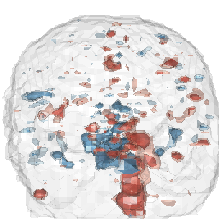
In this section we discuss two applications. One, on the analysis of CMB data, is discussed briefly at the end of the section. For a more detailed example, we return to the fMRI data discussed in the Introduction.
4.1 A fMRI example
We return to the language priming experiment of Dehaene-Lambertz et al. (2006) and apply our LKC regression method.
Contrary to the group-level comparison of Section 1, we conduct a within-subject study to identify stimulated regions for each specific individual. Here the stimulus refers to the difference in activation between the “different speaker” and “same speaker” conditions, under which each subject hears a sentence repeated twice either by two different speakers or by the same speaker. The subject is then scanned 191 times, alternatively undergoing the two stimuli. There are 14 such data sets, one for each individual, which are analyzed by Taylor and Worsley (2006) using the warping thresholding method. We reanalyze the data using our LKC regression method.
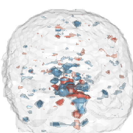
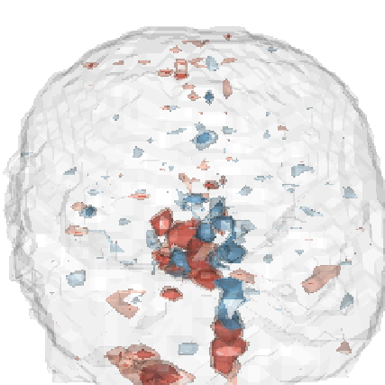
Prior to the analysis we conducted a standard preprocessing (Taylor and Worsley, 2006, as detailed in Section 2 of) of the data: First, a subject’s scans are aligned to correct for motion drift (Smith et al., 2004). An AR(1) time series model is then fitted to every voxel of the brain. The response variable is the fMRI activation level, which is a time series indexed by each of the 191 time points; in the AR(1) model, the stimulus effect is treated as a regression coefficient in front of a time-varying contrast that represents the level of stimulus administered at each time. There is one such model for every voxel in the brain; fitting all such models produces a random field of estimated stimulus effects across the brain: this is the field of interest, analogous to the field in Section 1. The random fields , correspond to the AR(1) residuals at every voxel and time. As in Section 1, the threshold is obtained from the and then applied to to identify regions where the stimulus effect is significant. There is one analysis — one and one set of — for every subject. As an example, three residual fields for the first subject in the study, corresponding to three separate time points, are shown in Figure 4.13. In Taylor and Worsley (2006), warping is used to estimate the threshold, which found values of around 5 for each subject.
We are interested in analyzing how these thresholds, found using warping (Taylor and Worsley, 2007), compare to those found using our proposed LKC regression method. For the purpose of such a comparison, the thresholds are estimated using warping and our LKC regression with smoothed diagonal (SD) covariance (which is found to be the best-performing option found in Section 3).
| 95% thres. | Runtime | |||||||||
|---|---|---|---|---|---|---|---|---|---|---|
| LKC | Warp | LKC | Warp | LKC | Warp | LKC | Warp | LKC | Warp | |
| 1 | 5.01 | 4.94 | 1,686 | 274 | 7,774 | 2,343 | 26,706 | 29,382 | 18.3 | 38.7 |
| 2 | 4.93 | 4.75 | 1,237 | -32 | 7,801 | 2,351 | 23,878 | 32,334 | 12.5 | 34.9 |
| 3 | 5.10 | 4.98 | 943 | 201 | 4,694 | 2,242 | 15,234 | 30,659 | 15.0 | 38.7 |
| 4 | 5.03 | 5.14 | 1,252 | 249 | 5,584 | 2,169 | 19,886 | 29,537 | 15.8 | 33.2 |
| 5 | 5.06 | 5.11 | 1,961 | 49 | 9,484 | 2,277 | 30,229 | 30,683 | 12.7 | 33.8 |
| 6 | 4.99 | 4.98 | 1,158 | 22 | 7,712 | 2,427 | 23,317 | 34,124 | 14.8 | 32.7 |
| 7 | 5.03 | 5.09 | 1,263 | 419 | 4,702 | 2,091 | 17,543 | 28,103 | 16.7 | 37.5 |
| 8 | 4.94 | 5.05 | 1,737 | 382 | 8,860 | 2,162 | 28,163 | 26,701 | 13.9 | 34.1 |
| 9 | 4.97 | 5.02 | 2,017 | 191 | 8,782 | 2,235 | 31,009 | 31,327 | 20.9 | 35.4 |
| 10 | 5.15 | 5.28 | 1,437 | 386 | 4,857 | 2,245 | 17,988 | 30,403 | 18.5 | 42.6 |
| 11 | 4.98 | 4.91 | 2,394 | 320 | 8,967 | 2,274 | 30,473 | 31,133 | 15.3 | 37.3 |
| 12 | 5.01 | 4.89 | 1,333 | 307 | 6,528 | 2,113 | 21,540 | 28,898 | 15.3 | 36.1 |
| 13 | 5.01 | 5.01 | 1,933 | 255 | 7,658 | 2,063 | 27,509 | 29,670 | 13.6 | 34.5 |
| 14 | 5.01 | 5.13 | 1,757 | 105 | 7,724 | 2,262 | 26,367 | 32,376 | 12.5 | 34.1 |
Table 3 compares the LKC estimates and the computational time of each method. The major difference is in the latter (rightmost column): the LKC regression is over twice as fast as warping. At first, while any improvement in computational speed is desirable, it would not seem that this improvement is all that important. Statistical analysis of fMRI data is typically done offline, as opposed to the actual production of fMRI data which is online and must be minimised for subject comfort and cost considerations.
Nevertheless, computation time is still an issue, as evidence by the fact that practitioners have developed data structures optimized for 3D fields (Theis and Tanaka, 2005, e.g.,) and schemes for parallel processing (Zhao et al., 2007; Wilde et al., 2009, e.g.,). Computational firepower is necessary because over the course of an fMRI study, the number of hypothesis tests conducted and thresholds found easily reaches into the hundreds. These computational demands occur for two reasons: first, there are usually multiple experimental stimuli, each with a categorical set of possible conditions (for instance, Taylor and Worsley (2006) consider three factors with two or three conditions each, yielding 12 significance analyses); and second, it is also common to perform subject-specific tests (one test per subject), or time-specific tests (one test per unit time) (Beckmann, Jenkinson and Smith, 2003, see). In light of these repeated computational demands that are inherent to various applications, our LKC regression can save substantial development time.
In addition to speed, accuracy also carries great importance for practictioners. As seen from the spread of the estimated 95% thresholds (leftmost column), LKC regression and warping produce very similar thresholds, with the mean values of the 14 subjects being 5.01 and 5.02, respectively. Thus, as to be expected, the activated regions change only slightly (not shown) and we are still able to reproduce the activation in the left and right mid-temporal gyri seen in Taylor and Worsley (2007).
What we have not yet checked in detail, but, from preliminary studies are quite certain is true, is that in higher dimensional problems the gain in speed of LKC regression over warping will be quite significant. What is definitely true is that the LKC approach, even in this three dimensional example, involves much less coding, since, following Section 3, it is basically just a regression analysis.
As a side note, it is interesting that the similarity in thresholds between LKC regression and warping belies often large differences in the estimated LKCs (middle three columns). These phenomena underscore the fact that different LKC combinations can lead to the same 95% thresholds, which are what matter in practice. It is impossible to tell which is correct because only the thresholds are observable, not the LKCs themselves. Interestingly, the discrepancies in and are not apparent in the cubic random field simulations of Section 3, where LKC regression and warping produce approximately the same LKC estimates. We suspect that isotropy plays a role: the simulated cubic fields are isotropic, while the FIAC data are likely anisotropic.
4.2 A cosmic microwave background radiation example
Working from an earlier version of the current paper, Fantaye et al. (2014) have used LKC regression to estimate the LKCs (‘Minkowski functionals’ in their language) for CMB fluctuation models.
To quote from their paper: “A general trend in modern cosmological research is the implementation of more and more sophisticated statistical tools to perform data analysis. Indeed, as well-known cosmological data have reached over the last decade an un- precedented accuracy, so that it has become customary to speak about a golden era for Cosmology, featuring a data deluge from a bunch of satellite - and ground based-experiments. As the data grow in size and precision, more and more detailed questions can be addressed, and exploiting techniques at the frontier of statistical and mathematical research becomes mandatory to warrant a full exploration of the available evidence.
Among these techniques, stochastic geometry tools have now become very well established, especially in the field of Cosmic Microwave Background radiation experiments. In this area, one of the most popular geometric tools for data analysis are certainly the so-called Minkowski functionals (MFs), which have been extensively exploited as tools to search for non-Gaussianities, anisotropies, asymmetries and other features of CMB data. The use of MFs in Cosmology goes back at least to [1, 2]; a complete bibliography would certainly include hundreds of entries, so we refer only to the earlier works by [3–10] and to the more recent ones by [11–16].” (References not included here.)
We recommend their paper, which contains detailed calculations and scientific discussions, as an excellent application of the techniques developed here (and, of course, for the many other things there).
5 Conclusion
We have presented a new method, the Lipschitz-Killing curvature regression, for estimating tail probabilities of a Gaussian random field. The LKC regression procedure is to estimate the Lipschitz-Killing curvatures and then substitute them into the Euler characteristic heuristic (1.4) to generate a threshold. The estimation does not require knowledge of the covariance structure of the field or even whether it is isotropic. It need not be Gaussian, although it must be Gaussian related. The high efficiency of our method hinges on the fact that the Euler characteristic can be well estimated from the data when the exceedence level is small or moderate. The LKC regression allows us to leverage the estimation strength at a low level for accurate approximation at high exceedence level.
The primary advantage of the LKC regression is its simplicity and speed. It is transparent, which offers straightforward interpretation, implementation, and diagnosis. It runs faster than its chief competitor, warping (Taylor and Worsley, 2007), with comparable accuracy. The key procedural difference is that LKC regression computes Euler characteristics of the input random fields, which is a fast computation when the sample sites lie on a grid. In practical terms, for the two- and three-dimensional random fields we considered, the gain in speed ranges from a factor of two to a factor of eight. It is most pronounced for high resolution fields, which are commonly found in practice. We believe that the gain rate will be considerably higher in higher dimensional cases, such as the scale-space (5D) of Siegmund and Worsley (1995) and the rotation-space fields (8D) of Shafie et al. (2003), for both of which the analytic evaluation of the LKCs is orders of magnitude harder than the isotropic cases we have considered in this paper (cf. Adler, Subag and Taylor (2012)).
Appendix
In this section we shall briefly discuss the Gaussian kinematic formula, which gives an exact formula for the expected Euler characteristic . We shall explain its general structure without going into technical details.
A.1 Gaussian and Gaussian related random fields
The basic building blocks of all the random fields we consider are smooth Gaussian random fields, or processes,
The first assumption that we place on , and the most important one, is that each of its components are twice differentiable, and that these derivatives are themselves continuous. Some additional minor assumptions of non-degeneracy also need to be made, but since these almost always hold in practice we direct the interested reader to Chapter 11 of Adler and Taylor (2007) or Chapter 4 of Adler, Taylor and Worsley (2015?) for details. For the rest of this paper we shall assume these conditions are met. The second assumption is a minor one, that all means be fixed at zero. A little more restrictively, we also assume that the have constant variance throughout . Note that this is a much weaker assumption than either isotropy or stationarity, which we do not require, and is achievable in general by replacing a random field that does not have constant variance by a normalized version of itself. Unless stated otherwise, for the remainder of this section we shall assume that this constant variance be 1. Finally, we assume that the components of are all independent and identically distributed.
Real valued Gaussian related random fields are defined by taking a smooth function and setting for all , where is as above. Gaussian related fields are typically quite different to Gaussian ones (for which and is the identity function). Three useful examples are given by the following choices for , where in the third we set .
| (A.1) |
The corresponding random fields are known as fields with degrees of freedom, the field with degrees of freedom, and the field with and degrees of freedom. These three random fields all have very different spatial behavior, and each is as fundamental to the statistical applications of random field theory as is its corresponding univariate distribution to standard statistical theory.
Throughout we shall assume that is twice continuously differentiable, and that for all real the sets are well behaved, as described in the following subsection. Under these conditions, Gaussian related fields are also twice continuously differentiable, with well behaved excursion sets.
A.2 Parameter spaces
The modern general theory of Gaussian fields, as developed in Adler and Taylor (2007), allows the parameter to be what is known as a Whitney stratified manifold, satisfying some mild side conditions. Roughly speaking, these are compact subsets of which can be written as a disjoint finite union
where is an -dimensional manifold (the open -dimensional ‘boundary’ of ).
An easy example is given by a -dimensional rectangle, in which is its interior, the collection of its (open) -dimensional faces, etc., down to which is the collection of its corners. If were a ball, we would decompose it into its interior, again , and its surface, the sphere .
The ‘Whitney’ part of the definition contains rules about how all the various pieces must be put together, and details can be found in Adler and Taylor (2007). More or less every (non-fractal) parameter space arising in statistical practice satisfies these rules.
A.3 The expected Euler characteristic of excursion sets
The Euler characteristic of a well behaved set is a topological invariant, that, typically, is easy to compute. For example, if is two-dimensional, then is simply the number of connected components in minus the number of holes. If is three-dimensional, then it is the number of components minus the number of handles plus the number of internal holes.
If is made up of a union of cubes, all of whose corners sit at the points of a rectangular lattice, then
where is the number of distinct facets of dimension in .
The central result behind this paper is then the following formula, which is a special case of a far more general result known as the Gaussian kinematic formula. (cf. Adler and Taylor (2007); Taylor (2006); Taylor and Adler (2003) for details.) It says that for Gaussian related field defined over well-behaving sets ,
| (A.2) |
The are the Lipschitz-Killing curvatures, or intrinsic volumes, of , and estimating these in statistical practice was one of the aims of this paper. If the are stationary and isotropic, and the variance of their first order partial derivatives is given by the second spectral moment , then where the are the Euclidean Lipschitz-Killing curvatures . The Euclidean Lipschitz-Killing curvatures are known under a variety of names, including Quermassintegrales, Minkowski or Steiner functionals, integral curvatures, and intrinsic volumes, the differences between them generally being of ordering and scaling. In general, can be thought of as a measure of the ‘-dimensional size’ of . For example, when , is the two dimensional area of , is half its boundary length, and its Euler characteristic. When , is the three-dimensional volume of , is half the surface area, is twice the caliper diameter of , (where the caliper diameter of a convex is defined by placing the solid between two parallel planes (or calipers), measuring the distance between the planes, and averaging over all rotations of ) and is again the Euler characteristic . In fact in all cases.
While these are simple examples of Lipschitz-Killing curvatures, when the underlying are not isotropic their covariance induces a Riemannian metric on , and the become quite complicated. To be a little more specific, they involve integrals of traces of powers of the curvature tensor and second fundamental forms, with respect to the volume form determined by the induced metric. In brief, these are not typically things that a practitioner wants to compute analytically, particularly since computing them also requires knowledge of the covariance function of the , something which typically needs to be estimated from data.
On the other hand, the functions in (A.2) are much easier to compute, and in many cases are given by
where and is a function determined by . In such cases, computing the is thus simply a matter of calculus, and for most interesting this has already been done. (Adler and Taylor (2007); Adler, Taylor and Worsley (2015?) have a number of useful examples with references to others.) A particularly simple example is given in the Gaussian case, in which, as mentioned above, and is the identity function. Then the are then given by
where , is the -th Hermite polynomial and
To give an example in a more complicated case, we consider the case, with degrees of freedom, so that is given by the leftmost function in (A.1). In this case, the are, for and ,
When ,
While this may look a little complicated, it is trivial to code, and the LKC regression procedure then continues as in the Gaussian case.
References
- Adler (1981) Adler, R. J. (1981). The Geometry of Random Fields. John Wiley & Sons Ltd., Chichester. Reprinted in 2010 by SIAM. MR82h:60103
- Adler (2000) Adler, R. J. (2000). On Excursion Sets, Tube Formulae, and Maxima of Random Fields. The Annals of Applied Probability 10 1–74.
- Adler, Subag and Taylor (2012) Adler, R. J., Subag, E. and Taylor, J. E. (2012). Rotation and Scale Space Random Fields and the Gaussian Kinematic Formula. Annals of Statistics 40 2910–2942.
- Adler and Taylor (2007) Adler, R. J. and Taylor, J. E. (2007). Random Fields and Geometry. Springer.
- Adler and Taylor (2011) Adler, R. J. and Taylor, J. E. (2011). Topological Complexity of Smooth Random Functions. Lecture Notes in Mathematics 2019. Springer, Heidelberg. Lectures from the 39th Probability Summer School held in Saint-Flour, 2009, École d’Été de Probabilités de Saint-Flour. [Saint-Flour Probability Summer School]. MR2768175
- Adler, Taylor and Worsley (2015?) Adler, R. J., Taylor, J. E. and Worsley, K. J. (2015?). Applications of Random Fields and Geometry: Foundations and Case Studies. Springer-Verlag In preparation, early chapters available at http://webee.technion.ac.il/people/adler/publications.html.
- Bardeen et al. (1986) Bardeen, J. M., Bond, J. R., Kaiser, N. and Szalay, A. S. (1986). The Statistics of Peaks of Gaussian Random Fields. Astrophysical Journal 304 15–61.
- Beckmann, Jenkinson and Smith (2003) Beckmann, C. F., Jenkinson, M. and Smith, S. M. (2003). General Multilevel Linear Modeling for Group Analysis in FMRI. Neuroimage 20 1052-1063.
- Cao and Worsley (1999) Cao, J. and Worsley, K. J. (1999). The Geometry of Correlation Fields With an Application to Functional Connectivity of the Brain. Annals of Applied Probability 9 1021–1057. MR2000k:60099
- Dehaene-Lambertz et al. (2006) Dehaene-Lambertz, G., Dehaene, S., Anton, J. L., Campagne, A., Ciuciu, P., Dehaene, G. P., Denghien, I., Jobert, A., LeBihan, D., Sigman, M., Pallier, C. and Poline, J. B. (2006). Functional Segregation of Cortical Language Areas by Sentence Repetition. Human Brain Mapping 27 360-371.
- Fantaye et al. (2014) Fantaye, Y., Hansen, F., Maino, D. and Marinucci, D. (2014). Cosmological Applications of the Gaussian Kinematic Formula. arxiv.org/pdf/1406.5420v1.pdf.
- Friston et al. (1994) Friston, K. J., Worsley, K. J., Frackowiak, R. S. J., Mazziotta, J. C. and Evans, A. C. (1994). Assessing the Significance of Focal Activations Using Their Spatial Extent. Human Brain Mapping 1 214–220.
- Gott et al. (2007) Gott, J. R., Colley, W. N., Park, C. G., Park, C. and Mugnolo, C. (2007). Genus Topology of the Cosmic Microwave Background From the WMAP 3-year Data. Monthly Notices of the Royal Astronomical Society 377 1668–1678.
- Gott et al. (2008) Gott, J. R., Hambrick, D. C., Vogeley, M. S., Kim, J., Park, C., Choi, Y. Y., Cen, R. and Ostriker, K. J. P. Nagamine (2008). Genus Topology of Structure in the Sloan Digital Sky Survey: Model Testing. Astrophysical Journal 675 16–28.
- Hall, Fisher and Hoffman (1994) Hall, P., Fisher, N. I. and Hoffman, B. (1994). On the Nonparametric Estimation of Covariance Functions. Annals of Statistics 22 2115-2134.
- Imiya and Eckhardt (1999) Imiya, A. and Eckhardt, U. (1999). The Euler Characteristics of Discrete Objects and Discrete Quasi-objects. Computer Vision and Image Understanding 75 307-318.
- Kilner and Friston (2010) Kilner, J. M. and Friston, K. J. (2010). Topological Inference for EEG and MEG Data. Annals of Applied Statistics 4 1272-1290.
- Loader (1999) Loader, C. (1999). Local Regression and Likelihood. Springer, New York.
- Loader (2010) Loader, C. (2010). locfit: Local Regression, Likelihood and Density Estimation R package version 1.5-6.
- Mantoglou and Wilson (1982) Mantoglou, A. and Wilson, J. L. (1982). The Turning Bands Method for Simulation of Random Fields Using Line Generation by a Spectral Method. Water Resources Research 18 1379-1394.
- Pukelsheim (2006) Pukelsheim, F. (2006). Optimal Design of Experiments. Society for Industrial and Applied Mathematics.
- Rao (1962) Rao, C. R. (1962). A Note on a Generalized Inverse of a Matrix With Applications to Problems in Mathematical-statistics. Journal of the Royal Statistical Society Series B-Statistical Methodology 24 152-158.
- Sampson and Guttorp (1992) Sampson, P. and Guttorp, P. (1992). Nonparametric Estimation of Nonstationary Spatial Covariance Structure. Journal of the American Statistical Association 87 108-119.
- Schlather (2009) Schlather, M. (2009). RandomFields: Simulation and Analysis of Random Fields R package version 1.3.41.
- Shafie et al. (2003) Shafie, K., Sigal, B., Siegmund, D. and Worsley, K. J. (2003). Rotation Space Random Fields With an Application to fMRI Data. Annals of Statistics 31 1732–1771.
- Siegmund and Worsley (1995) Siegmund, D. O. and Worsley, K. J. (1995). Testing for a signal with unknown location and scale in a stationary Gaussian random field. Ann. Statist 23 608–639.
- Smith et al. (2004) Smith, S. M., Jenkinson, M., Woolrich, M. W., Beckmann, C. F., Behrens, T. E. J., Johansen-Berg, H., Bannister, P. R., De Luca, M., Drobnjak, I., Flitney, D. E., Niazy, R. K., Saunders, J., Vickers, J., Zhang, Y. Y., De Stefano, N., Brady, J. M. and Matthews, P. M. (2004). Advances in Functional and Structural MR Image Analysis and Implementation as FSL. Neuroimage 23 S208-S219.
- Taylor (2006) Taylor, J. E. (2006). A Gaussian kinematic formula. Annals of Probability 34 122-158.
- Taylor and Adler (2003) Taylor, J. E. and Adler, R. J. (2003). Euler characteristics for Gaussian fields on manifolds. Annals of Probability 31 533–563.
- Taylor, Takemura and Adler (2005) Taylor, J. E., Takemura, A. and Adler, R. J. (2005). Validity of the Expected Euler Characteristic Heuristic. Annals of Probability 33 1362–1396. MR2150192 (2006b:60073)
- Taylor and Worsley (2006) Taylor, J. E. and Worsley, K. J. (2006). Inference for Magnitudes and Delays of Responses in the FIAC Data Using BRAINSTAT/FMRISTAT. Human Brain Mapping 27 434-441.
- Taylor and Worsley (2007) Taylor, J. E. and Worsley, K. J. (2007). Detecting Sparse Signals in Random Fields, With an Application to Brain Mapping. Journal of the American Statistical Association 102 913-928.
- Theis and Tanaka (2005) Theis, F. J. and Tanaka, T. (2005). A fast and efficient method for compressing fMRI data sets. In Artificial Neural Networks: Formal Models and Their Applications - ICANN 2005, Pt. 2, Proceedings, ( Duch, W and Kacprzyk, J and Oja, E and Zadrozny, S, ed.). Lecture Notes in Computer Science 3697 769-777.
- Torres (1994) Torres, S. (1994). Topological Analysis of COBE-DMR Cosmic Microwave Background Maps. Astrophysical Journal 423 9–12.
- Vogeley et al. (1994) Vogeley, M. S., Park, C., Geller, M. J., Huchin, J. P. and Gott, J. R. (1994). Topological Analysis of the CfA Redshift Survey. Astrophysical Journal 420 525–544.
- Wilde et al. (2009) Wilde, M., Foster, I., Iskra, K., Beckman, P., Zhang, Z., Espinosa, A., Hategan, M., Clifford, B. and Raicu, I. (2009). Parallel Scripting for Applications at the Petascale and Beyond. Computer 42 50-60.
- Worsley (1994) Worsley, K. J. (1994). Local Maxima and the Expected Euler Characteristic of Excursion Sets of and Fields. Advances in Applied Probability 26 13–42. MR94i:60064
- Worsley (1995a) Worsley, K. J. (1995a). Boundary Corrections for the Expected Euler Characteristic of Excursion Sets of Random Fields, With an Application to Astrophysics. Advances in Applied Probability 27 943–959. MR97b:60068
- Worsley (1995b) Worsley, K. J. (1995b). Estimating the Number of Peaks in a Random Field Using the Hadwiger Characteristic of Excursion Sets, With Applications to Medical Images. Annals of Statistics 23 640–669.
- Zhao et al. (2007) Zhao, Y., Hategan, M., Clifford, B., Foster, I., von Laszewski, G., Nefedova, V., Raicu, I., Stef-Praun, T. and Wilde, M. (2007). Swift: Fast, Reliable, Loosely Coupled Parallel Computation. IEEE Congress on Services 0 199-206.