Consensus measure of rankings
Abstract
A ranking is an ordered sequence of items, in which an item with higher ranking score is more preferred than the items with lower ranking scores. In many information systems, rankings are widely used to represent the preferences over a set of items or candidates. The consensus measure of rankings is the problem of how to evaluate the degree to which the rankings agree. The consensus measure can be used to evaluate rankings in many information systems, as quite often there is not ground truth available for evaluation.
This paper introduces a novel approach for consensus measure of rankings by using graph representation, in which the vertices or nodes are the items and the edges are the relationship of items in the rankings. Such representation leads to various algorithms for consensus measure in terms of different aspects of rankings, including the number of common patterns, the number of common patterns with fixed length and the length of the longest common patterns. The proposed measure can be adopted for various types of rankings, such as full rankings, partial rankings and rankings with ties. This paper demonstrates how the proposed approaches can be used to evaluate the quality of rank aggregation and the quality of top- rankings from Google and Bing search engines.
I Introduction
In many information systems, rankings are widely used to represent the preferences over a set of items or candidates, ranging from information retrieval, recommender to decision making systems [1, 2, 3, 4, 5, 6], in order to improve quality of the services provided by the systems. For example, in search engine, the list of the terms suggested by a search engine after a user’s few keystrokes is a typical ranking and such ranking service, widely adopted nowadays, has great impact on user’s search experience; it is also recognized that the list of search results is a ranking after a query is issued.
A ranking is an ordered sequence of items, in which an item with higher ranking score is more preferred than the items with lower ranking scores. The consensus of rankings is the degree to which the rankings agree according to certain common patterns. The consensus measure, can be used in many information systems, in order to uncover how close or related the rankings are. For example, in the group decision making, a group of experts express their preferences over a set of candidates by using rankings and the measure of the degree of consensus is very useful for reaching consensus [2].
In many information system with large volume of items, such as search engines, it is hard to clearly define what ground truth is, which make it more difficult to evaluate and compare the rankings returned from the systems. The consensus measure of rankings, as a tool for understanding how related or close the rankings are, will help engineers and researchers to discern what aspects of a ranking system need to be improved and to detect outliers [7, 8]. For a set of rankings , one approach to understanding the degree to which rankings agree is to use rank correlation or similarity function by pairwise comparison [3, 9, 10, 11, 12, 13, 14, 15, 16]. The notable functions include the Kendall index and the Spearman index [12, 14], which however do not have a weighting scheme so that less important items can be penalized. It is common that in information retrieval, the documents (items) at the top of a ranking list are more important than those at the bottom [17]. As such, it makes sense to reduce the impact from the bottom items with a weighting scheme. For example, the variation of index, denoted by , with average precision, is able to give greater weight to the top items of the ranking lists [9]. These methods assume rankings are conjoint, meaning that items in the rankings are completely overlapped. Undoubtedly, they cannot be used for partial rankings, in which items may not be mutually overlapped. As a similarity function for two partial rankings, the RBO (rank-biased overlap) proposes to weight the number of common items according to the depth of rankings [15], and it doesn’t take into account the order of items in the rankings.
When one of the correlation or similarity functions is used for consensus measure for a set of rankings in , we can aggregate the pairwise comparison values across all rankings for times. Since the pairwise comparison is based on the degree of commonality in two rankings, with respect to features or patterns (e.g, the common items, or the concordant pairs against the disconcordant pairs), the aggregated result is not informative enough to tell the extend to which the rankings agree in , according to the study by Elzinga et al. [18]. Also, the type of rankings can be full or partial, specially the top- [17], the existing measures fail to meet the requirements for handling different types of rankings.
In order to effectively evaluate and compare rankings, which could be full or partial and especially in which some items need to be weighted, this paper propose a new approach based on graph representation. The novelty of this paper lies in that fact the new proposed consensus measure of rankings does not need pairwise comparison, which is significantly different from the pairwise approaches using similarity or correlation functions. The contribution of the paper includes:
- •
we introduce a directed acyclic graph (DAG) to represent the relationship between items in the rankings so that such representation can be used to induce efficient algorithms for consensus measure of rankings;
- •
the proposed representation of DAG enables us to approach consensus measure of rankings in terms of different aspects of the common features or patterns hidden in the rankings, including – the number of common patterns, – the number of common patterns with a fixed length , and – the length of the longest or largest common patterns.
- •
the proposed representation of DAG is extended to allow the edges in the graph to have weights so that more “important” features or patterns are assigned with higher values and the features or patterns with less “importance” are penalized.
- •
we also demonstrate that the consensus measure of rankings with graph representation can be extended to calculate consensus measure for duplicate rankings, for rankings with ties and for rankings whose top items need to be weighted.
- •
we show that our approach can be used for different types of rankings, including the full rankings and top- rankings.
The rest of paper is organized as follows. Section II introduces the important notations and concepts used in the paper, followed by a review of related work in Section III. Section IV presents a directed graph representation approach for consensus measure. Section V shows how the proposed approaches can be used to evaluate rank aggregation and to compare top- rankings. The paper is concluded in Section VI.
II Preliminaries
This section introduces notations and concepts of graph, ranking sequence, and consensus measure that will be used in the rest of the paper.
II-A Directed graph
A directed graph is a pair , where is the set of nodes (or vertices) and is the set of directed edges. A directed edge means that the edge leaves node and enters node . An edge is called a loop, which leaves node and returns to itself. Given a graph with nodes, matrix is used to denote the adjacency matrix of graph , where if there exists edge ; and , otherwise.
The adjacency matrix assumes that all the edges have identical weights of 1, and this can be relaxed in the weighted directed graph. A weighted directed graph is a directed graph, in which is a set of weights on the edges and each edge is assigned a non-zero weight . Then, the adjacency matrix for is defined as if and , otherwise.
A path from node to is a sequence of distinct non-loop edges
connecting node and .
II-B Ranking sequences
A ranking is an ordered sequence of distinct items drawn from a universe , where and is more preferred than if . The length of is denoted by . For notational simplicity, we shall simply write a ranking as a sequence of in the rest of the paper.
For a ranking , where for , we can define the embedded patterns with respect to subsequences. A sequence is called a subsequence of , denoted by , if can be obtained by deleting items from . We denote by that is not a subsequence of . For example, , and .
A ranking sequence with no items is an empty sequence. We use to denote the set of all possible non-empty subsequences of . can be partitioned into subsets , where consists of all subsequences of length . For example, if , then , in which each subsequence has length .
The degree to which rankings agree lies in the common patterns or features which are embedded in the rankings. For ranking sequences, the subsequences are the patterns or features. Given a set of rankings , consider , each element is a common subsequence of , for which we also use the notation . Similar to , we also define to denote the subsets of all common subsequences of length . Therefore, it holds that , where . In a special case, for two rankings and , we will write to denote the set of -long common subsequences between and .
It is clear that accommodates all common features (subsequences), which are subsumed by each ranking . Let denote the number of all common subsequences of , i.e,
| (1) |
The more common features has or the bigger is, the higher degree of consensus has. We also define
| (2) |
in order to measure the consensus in with respect to the number of subsequences of a given length . The length of the longest common subsequences of rankings in is denoted by or simply . Then, .
Therefore, we have the following properties:
- •
For a set with only one ranking , where , ;
- •
For a set of two rankings , where and , we have
- •
For two sets of rankings and , if , then
(3)
II-C Consensus measure of rankings in feature spaces
For a set of rankings , we can form a set of features . Let and . Each ranking can be represented by a feature vector with a mapping function :
where
| (4) |
It is clear that , defined in Equation (1) can be rewritten using the inner product on -inner product spaces [19, 20] as
| (5) |
With the generalized inner product, we find that the is a kernel function [21] when . The rewritten relies on the definition of as defined in Equation (4), whose co-domain is . It is computationally expensive to enumerate all the features and to form . In this section, we will transform relationship between items to a graph so that efficient algorithms can be found without enumerating features explicitly, which is similar to the kernel trick for kernel functions [21].
III Related work
A ranking can be full or partial ranking, depending on the number of items from being ranked. A ranking is a full ranking if . A ranking is called partial ranking if the items in forms a subset of . A top- ranking is a sub-ranking of full ranking but only with the top- items. Rankings with ties occur when some items share an identical ranking score, which happens very often in the decision making or voting process [16]. For example, in a ranking , both items and are assigned with an identical ranking score.
Evaluation or comparison of rankings is an important tasks in many ranking related systems, including decision making, information retrieval, voting and recommender [1, 2]. One approach to evaluating rankings is to use rank correlation between two rankings. The widely used Kendall index [12, 13] is a measure of rank correlation between two rankings and over items by taking into account 2-long common subsequences between them, which can be formulated as
where is a reverse ranking of . In rank aggregation, one could also use the Kendall distance – a variation of the Kendall :
The Spearman index is another measure of rank correlation that does not utilize the 2-long common subsequences but instead takes into account of each item positions in and [14]. It is defined as follows
where . The Spearman footrule distance is an distance, which is a variation of the Spearman :
Compared with the Spearman , the Kendall ignores the use of items positions, which are in many cases very important factors, e.g, for the top- rankings. Again, the Spearman can not be used for sensitivity detection and analysis, as studied in [13].
Both Kendall and Spearman can only be used for full rankings. They cannot be used for partial or top- rankings. Even in full rankings, both of them lack of weighting schemes and are not flexible enough for rankings whose items at the top are more important than the items at the bottom [17]. Therefore, it is necessary to reduce the impact from the bottom items with a down-weighting scheme for those bottom items. For example, the variation of index, denoted by , with average precision, is able to give greater weight to the top items of the ranking lists [9]. Shieh also developed a weighted metric based on the Kendall by adding weighting factors to the 2-long subsequences [22]. For full rankings with ties, was proposed based on the Kendall index [16]. One extension to the Spearman index by Iman et al. was to assign higher weights to the items at the top [23].
The above methods assume that rankings are full rankings, meaning that items in the rankings are completely overlapped. Therefore, they cannot be used for partial rankings. In information retrieval, it is more interesting to compare the the rankings based on their top- items. Fagin et al. proposed two measures and by adapting both Kendall and Spearman for top- rankings [17]. As a similarity function for two partial rankings, the RBO (rank-biased overlap) proposes to weight the number of common items according to the depth of rankings [15], but it does not take into account the order of items in the rankings.
| Full | Partial | Weighted | Ties | |
| x | ||||
| x | ||||
| x | x | |||
| x | x | |||
| x | x | |||
| x | ||||
| RBO | x | x | ||
| x | x | |||
| x | x | x | x | |
| x | x | x | x |
These functions are pairwise comparison and they can be transferred into consensus measure for a set of rankings by aggregating the pairwise distance values across all rankings. For example, one can use if the Kendall index is preferred. However, this aggregated result is not informative enough to tell the extend to which the rankings agree in , according to the study by Elzinga et al. [18].
We summarize the popularly used indices in Table I and we show that our approach of and is more flexible for various types of rankings, which will be demonstrated in the next section. Also, those existing indices shown in Table I cannot be used for sensitivity detection in the consensus measure, while our approach has the ability to discern how the rankings come to agree by varying the parameters to the gaps and positions of items, as pointed out in Section IV-D1 and as verified in Section V.
IV Graph representation for consensus measure of rankings
This section will introduce a graph approach to consensus measure of rankings by calculating and .
IV-A A motivating example
Consider a set of rankings . Without loss of generality, we randomly pick (note that ) and form a lower triangle matrix of size , where for , if the item and the item of both occur in the same order in all rankings in , and otherwise. Then we obtain matrix :
| (6) |
With matrix , we can induce a weighted directed graph on the diagonal elements of , where is the set of vertices, is the set of loops and is the set of non-loop edges. Later, we may use interchangeably without confusion as each stands for an item. Hereinafter in this paper, we shall distinguish loops and non-loops edges, and abuse the notation and simply call the latter edges.
The edges are drawn according to the following: for , an edge from to is added if the following conditions all hold: (1) ; (2) ; (3) . We also add dashed loops on diagonal elements of value . Figure 1 shows the weighted directed graph for the matrix , in which there are seven directed (solid) edges, i.e,
or simply Those edges are the 2-long common subsequences: , and all of them occur in , , and . As such, . Similarly, paths11 1 Recall that our definition of path excludes loop edges. of length corresponds to common subsequences of length . We find that with common subsequences being , , and . Next, with the common subsequence being . There is no longer common subsequences since the length of the longest path in is .
In Figure 1, the five dashed loops mean five singletons, i.e., , , , , . As a result, . Therefore, we obtain .
This process of finding patterns of various lengths with graph representation not only allows us to calculate , but also makes it easy for us to calculate the number of all common patterns and the length of the longest common subsequences .
IV-B Consensus measure by graph representation
The above example shown in Fig. 1 presents an approach with graph representation for consensus measure of rankings when . This section will extends the graph representation to the consensus measure of rankings by calculating and , when .
In Equation (4), the definition of assumes that features in are equally assigned with a weight of 1. However, this is not true in many cases when some features or items in is more important than the others [9, 15]. The definition of is not flexible enough to differentiate the importance of the features. As such, we shall extend it to if , and if so that “important” features will receive higher values of while features with less importance will be “penalized” with lower . Therefore, we rewrite Equation (5) as
| (7) |
for .
In the DAG shown in Figure 1, we assume that the weights on the edges equal to 1, which does not reflect the nature of how each subsequence is embedded in the original rankings. Consider the four rankings in , item occurs at different positions in the rankings, which is shown in the following table:
| 6 | 5 | 10 | 5 |
The position for in is 10, which deviates from the positions of in the other rankings substantially. In order to incorporate those factors which may affect the degree of consensus, we relax the assumption that the weights are identical to 1 and generalize the induced weighted DAG by introducing two functions and . Figure 2 shows the new DAG, where each edge is associated with weight and each loop is assigned with , where and . We will illustrate how the two functions reflect those factors in the following sections, and how they are related to for Equation (7).
For simpler presentation of our algorithm, we introduce the (left-continuous) Heaviside function
| (8) |
Now we present the following theorem for measuring the consensus of rankings.
Theorem 1.
Given a set of rankings over a universe , where each ranking is naturally associated with a map defined as
| (9) |
Let be an arbitrary ranking from , , and be an adjacency matrix of a graph, where
| (10) |
and let be strictly lower triangle of , and be a vector of all ones. Then,
| (11) |
Proof.
Note that gives the sum of all entries in a matrix . By definition of we know that if and otherwise. It follows that is the number of s on the diagonal line, which equals to, noting that all other entries on the diagonal lines are s, the sum of diagonal entries of , or .
For , it is a classical inductive argument that when , where is the number of common sequences of length which begin with and end with . The advertised result then follows from the fact that all rankings have distinct items and thus the common subsequences also have distinct items. ∎
Theorem 1 shows that the individual items are weighted by and the edges between any two items by , reflecting the strength of the relationship between two items and .
IV-B1 – weighted by standard deviation of item’s positions
The position of item in a ranking is an indication of the strength of being preferred. To show the importance of the position of , we define , the average of the positions of in , as follows.
| (12) |
If an item is placed in a small range of positions throughout all rankings, it is assumed that this item is preferred consistently at the same level by all rankings. On the other hand, if an item has a low position in one ranking while has a high position in another ranking , the big difference between the positions indicates the inconsistency of the preferences over this item. To take into account the differences of item’s positions in consensus measure, we define
| (13) |
where , in order to weigh the item using the positions . In fact, when feature is a singleton (i.e., ), it is clear that
where for Equation (7).
IV-B2 – weighted by gaps
The gap between items has been used for pairwise kernel functions or sensitivity detection [24, 21]. Now we extend this to the set-wise consensus measure of .
The weighted DAG in Figure 2 shows that the edges and , i.e., subsequences and are quite different in terms of the distance between and , and between and , in . There are no items between and , however and are separated by three other items , and , which means that is much more preferred than . Therefore, for each and every 2-long subsequence , we define the gap , which indicates how much is more preferred than its successor in the 2-long subsequence with respect to the original ranking sequence . The following table shows the gaps for and with respect to the example rankings.
| 1 | 2 | 1 | 5 | |
| 4 | 4 | 9 | 4 |
Clearly, the accumulated gaps for and is much bigger than that for and . This suggests that is less likely to be preferred over . To take into account this likelihood, we define
| (14) |
where and , so that any subsequence with bigger average gaps will be “penalized”.
IV-B3 An example for and
Comparing Fig. 1 and Fig. 2, obviously the example in Section IV-A is a special case for Theorem 1 when and .
Example 1.
IV-C and
In Example 1, we observe that for , which implies that there are no common subsequences with length more than 4 and hence the length of the longest common subsequences of is 4. Based on this fact, the following corollary of Theorem 1 provides an algorithm for calculating .
Corollary 1.
Under the assumptions in Theorem 1 , the length of the longest subsequences in can be obtained by
Corollary 2.
Under the assumptions in Theorem 1 ,
where and is the identity matrix of size . Consequently can be computed in time.
Proof.
Since the longest possible length of a common subsequence is , Theorem 1 implies that
Invoking the identity and the observation that since is strictly lower triangular, we obtain that
| (15) | |||||
Now we discuss the runtime. Since is a strictly lower triangular matrix, is lower triangular. Note that computing is equivalent to solving and, if is lower triangular, can be done efficiently in time using forward elimination (degenerated Gaussian elimination), where denotes the number of non-zero entries in . Therefore can be computed in time, and thus in time. ∎
We remark that the runtime in Corollary 2 is significantly faster, by a factor of , than the naïve algorithm to sum up over , which would take time.
IV-D Remarks
Algorithm 1 is the pseudocode for Theorem 1. Generating (Line 1–1) takes time. Computing (Line 1) takes time. For each , the matrix-vector multiplication in Line 1 takes time, since has at most non-zero entries. In fact, . Line 20 takes time. Overall computing , after generation of , takes time for .
IV-D1 Sensitivity detection by gaps and positions of items
There are some differences among . Note that is controlled by the and in Equation (13), where is a factor to reflect the deviation of each item’s positions in the rankings. Higher disagreement of the items positions in the rankings will result in lower . Hence is sensitivity detection of the variation of items positions. Whereas for , the measure takes into account the extent of the relationship between two items by incorporating and in Equation (14).
We demonstrate such ability for sensitivity detection in terms of the gaps and positions of items in Section V.
IV-D2 Duplicate rankings
In the above example of and its adjacent matrix in Equation (6), we assume that there are only distinct rankings in . However, this is not the case, especially in the group decision making process, where there may be duplicate rankings produced by the experts. For example, we may have a multi-set , , which contains duplicate ranking of . Obviously, has higher degree of consensus than . However, as , that is, cannot discriminate and . In order to distinguish the difference, we let be the number of occurrences of ranking in , and define
where and is the set of all distinct rankings in .
IV-D3 Rankings with ties
Rankings with ties occur when the preference scores over some items are identical. Let be a ranking with ties, where is a set of items with an identical ranking score, if , and for , every is more preferred than all . If we replace Equation (9) with
| (16) |
then Theorem 1 can be used, without any modification, to measure consensus of rankings with ties.
IV-D4 Weighting scheme for top- items
The measure is a subsequence-based consensus measure and has the ability to handle top- rankings. In the case where the top- items rankings need to be weighted with greater value and the items after top- are not important (see, e.g. [9, 15, 17]), a slight revision to Equation (13) will accommodate this. Consider a given cut-off value for items position, we can weigh the items with
where . Clearly, if an items is ranked after position in one of the rankings, .
V Experiments
This section will present how the proposed and can be applied to evaluate rank aggregation and compare search engine rankings. The source codes and the experimental data used are available on the github repository 33 3 https://github.com/zhiweiuu/secs.
V-A Evaluation of rank aggregation of full rankings
| Validation | – The set of rankings for clustering algorithms | |||||||||
|---|---|---|---|---|---|---|---|---|---|---|
| measures | 1 | 2 | 3 | 4 | 5 | 6 | 7 | 8 | 9 | 10 |
| APN | SM | FN | ST | KM | PM | HR | AG | CL | DI | MO |
| AD | SM | FN | KM | PM | CL | ST | DI | HR | AG | MO |
| ADM | FN | SM | ST | KM | CL | PM | DI | HR | AG | MO |
| FOM | SM | CL | KM | PM | FN | ST | DI | HR | AG | MO |
| Connectivity | HR | AG | DI | KM | MO | SM | FN | CL | PM | ST |
| Dunn | HR | AG | KM | PM | DI | SM | CL | MO | FN | ST |
| Silhouette | HR | AG | KM | SM | CL | PM | ST | DI | FN | MO |
| Algorithm | Aggregation results | |||||||||
|---|---|---|---|---|---|---|---|---|---|---|
| GA | SM | HR | KM | FN | AG | PM | CL | DI | ST | MO |
| CE | KM | SM | PM | FN | HR | AG | CL | DI | ST | MO |
| CE | |||||||||||||
|---|---|---|---|---|---|---|---|---|---|---|---|---|---|
| 1 | 0.95 | 0.9 | 0.85 | 0.8 | 0.75 | 0.7 | 0.65 | 0.6 | 0.55 | 0.5 | 0.45 | ||
| 1 | 19 | 17.589 | 16.376 | 15.336 | 14.448 | 13.692 | 13.05 | 12.508 | 12.05 | 11.666 | 11.344 | 11.076 | |
| 0.95 | 17.945 | 16.534 | 15.321 | 14.282 | 13.394 | 12.637 | 11.996 | 11.453 | 10.996 | 10.611 | 10.29 | 10.021 | |
| 0.9 | 16.964 | 15.553 | 14.34 | 13.301 | 12.413 | 11.657 | 11.015 | 10.472 | 10.015 | 9.631 | 9.309 | 9.04 | |
| 0.85 | 16.055 | 14.644 | 13.431 | 12.391 | 11.503 | 10.747 | 10.105 | 9.563 | 9.105 | 8.721 | 8.399 | 8.13 | |
| 0.8 | 15.213 | 13.803 | 12.589 | 11.55 | 10.662 | 9.906 | 9.264 | 8.721 | 8.264 | 7.88 | 7.558 | 7.289 | |
| 0.75 | 14.438 | 13.027 | 11.814 | 10.775 | 9.886 | 9.13 | 8.489 | 7.946 | 7.489 | 7.104 | 6.782 | 6.514 | |
| 0.7 | 13.726 | 12.315 | 11.102 | 10.063 | 9.174 | 8.418 | 7.777 | 7.234 | 6.777 | 6.392 | 6.07 | 5.802 | |
| 0.65 | 13.075 | 11.664 | 10.451 | 9.411 | 8.523 | 7.767 | 7.125 | 6.583 | 6.125 | 5.741 | 5.419 | 5.151 | |
| 0.6 | 12.482 | 11.071 | 9.858 | 8.818 | 7.93 | 7.174 | 6.532 | 5.99 | 5.532 | 5.148 | 4.826 | 4.557 | |
| 0.55 | 11.944 | 10.533 | 9.32 | 8.281 | 7.392 | 6.636 | 5.995 | 5.452 | 4.995 | 4.61 | 4.288 | 4.02 | |
| 0.5 | 11.46 | 10.049 | 8.836 | 7.796 | 6.908 | 6.152 | 5.51 | 4.967 | 4.51 | 4.126 | 3.804 | 3.535 | |
| 0.45 | 11.026 | 9.615 | 8.402 | 7.362 | 6.474 | 5.718 | 5.076 | 4.533 | 4.076 | 3.692 | 3.37 | 3.101 | |
| GA | |||||||||||||
| 1 | 0.95 | 0.9 | 0.85 | 0.8 | 0.75 | 0.7 | 0.65 | 0.6 | 0.55 | 0.5 | 0.45 | ||
| 1 | 19 | 17.534 | 16.28 | 15.211 | 14.303 | 13.536 | 12.889 | 12.346 | 11.892 | 11.514 | 11.201 | 10.942 | |
| 0.95 | 17.966 | 16.5 | 15.246 | 14.177 | 13.27 | 12.502 | 11.855 | 11.312 | 10.859 | 10.481 | 10.167 | 9.908 | |
| 0.9 | 17.007 | 15.541 | 14.287 | 13.218 | 12.31 | 11.543 | 10.896 | 10.353 | 9.899 | 9.521 | 9.208 | 8.949 | |
| 0.85 | 16.119 | 14.653 | 13.399 | 12.33 | 11.422 | 10.655 | 10.008 | 9.465 | 9.011 | 8.634 | 8.32 | 8.061 | |
| 0.8 | 15.3 | 13.834 | 12.58 | 11.511 | 10.603 | 9.835 | 9.189 | 8.646 | 8.192 | 7.814 | 7.501 | 7.242 | |
| 0.75 | 14.546 | 13.08 | 11.826 | 10.757 | 9.85 | 9.082 | 8.435 | 7.892 | 7.439 | 7.061 | 6.747 | 6.488 | |
| 0.7 | 13.856 | 12.39 | 11.136 | 10.066 | 9.159 | 8.391 | 7.744 | 7.202 | 6.748 | 6.37 | 6.057 | 5.797 | |
| 0.65 | 13.225 | 11.759 | 10.505 | 9.436 | 8.528 | 7.76 | 7.114 | 6.571 | 6.117 | 5.739 | 5.426 | 5.167 | |
| 0.6 | 12.651 | 11.186 | 9.931 | 8.862 | 7.955 | 7.187 | 6.54 | 5.997 | 5.544 | 5.166 | 4.852 | 4.593 | |
| 0.55 | 12.132 | 10.666 | 9.412 | 8.343 | 7.435 | 6.668 | 6.021 | 5.478 | 5.025 | 4.647 | 4.333 | 4.074 | |
| 0.5 | 11.664 | 10.199 | 8.944 | 7.875 | 6.968 | 6.2 | 5.553 | 5.011 | 4.557 | 4.179 | 3.865 | 3.606 | |
| 0.45 | 11.245 | 9.779 | 8.525 | 7.456 | 6.549 | 5.781 | 5.134 | 4.591 | 4.138 | 3.76 | 3.446 | 3.187 | |
Rank aggregation, with wide applications in decision making systems, machine learning and social science, is the problem of how to combine many rankings in order to obtain one consensus ranking [25, 2]. Dwork et al. has proved that, even if , obtaining an optimal aggregation with the Kendall index is NP-hard [26]. Another problem with rank aggregation is the lack of ground truth for evaluation. Here, we show how we can use the proposed to evaluate the ranking aggregation results.
The rankings used in this experiment are the seven rankings (shown in Table II) of 10 clustering algorithms with respect to 7 different validation measures when they are used to cluster microarray data into five clusters [27]. The details for the 7 validation measures of APN, AD, ADM, FOM, connectivity, Dunn and Silhouette and the details for 10 clustering algorithms of SM, FN, KM, PM, HR, AG, CL, DI and MO can be found in [27]. Here, we use to denote the set of the 7 rankings. Two rank aggregation algorithms (the Cross-Entropy Monte Carlo algorithm (CE) and the Genetic algorithm (GA) ) have been used to aggregate the 7 rankings in [27] and the aggregated rankings are shown in Table III. We create two sets of rankings and by adding each aggregated ranking into ,
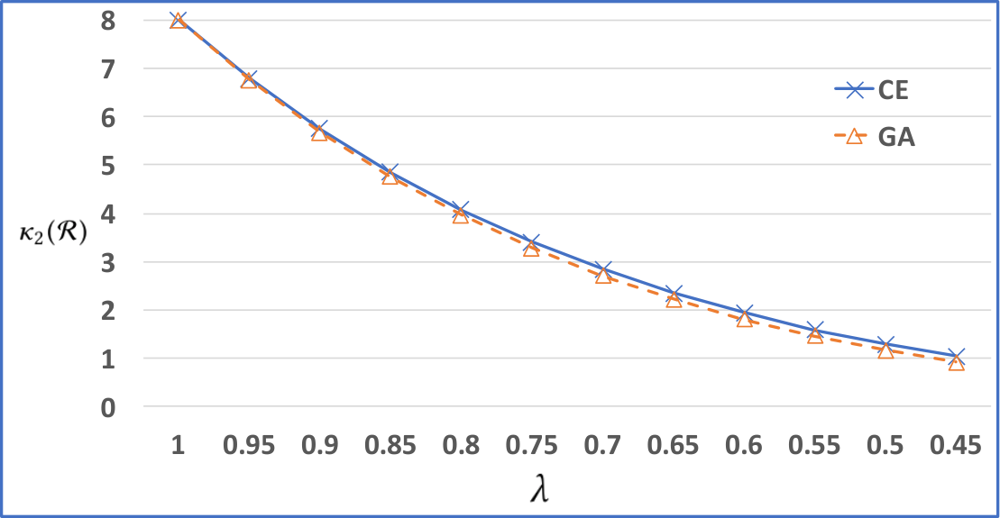
Based on the property in Equation (3), clearly and . Therefore, we would reasonably expect that a better aggregated ranking would result less decline of when adding the aggregated ranking into . Table IV shows experimental results for and by varying values of and from 1 to 0.45. Figure 3 shows the changes of for both GA and CE. We find that the aggregated ranking by the CE algorithm is more sensitive to while the aggregated ranking by the GA algorithm is more sensitive to .


V-B Evaluation of consensus for top- rankings
| Top 25 links from Google | |
|---|---|
| 0,68,9,59,11,5,3,69,79,70,21,4,36,32,76,40,60,51,80,81,42,29,82,83,73 | |
| 5,0,9,11,59,76,3,36,21,79,90,70,4,60,93,35,50,40,42,92,86,87,73,98,94 | |
| 0,9,11,5,3,59,70,84,85,21,76,4,32,42,51,62,12,80,67,60,55,86,87,73,29 | |
| 0,9,3,11,5,2,59,4,32,21,60,35,42,61,62,12,51,17,63,64,55,65,66,40,67 | |
| 5,0,68,9,3,11,59,69,70,71,4,21,60,32,36,61,65,72,73,58,74,75,76,77,78 | |
| 0,9,59,5,11,3,88,60,89,69,90,70,32,91,75,92,93,94,61,40,86,87,95,96,97 | |
| Top 25 links from Bing | |
| 0,9,1,11,36,8,4,2,22,5,37,15,38,6,28,34,29,19,39,40,35,24,41,32,42 | |
| 0,1,9,2,11,5,50,8,4,56,57,22,3,40,51,7,41,15,19,37,36,55,42,58,38 | |
| 0,7,9,2,10,8,4,6,5,1,11,14,3,40,13,43,19,44,45,46,47,48,49,17,28 | |
| 0,1,2,3,4,5,6,7,8,9,10,11,12,13,14,15,16,17,18,19,20,21,22,23,24 | |
| 9,1,25,4,7,2,0,26,5,11,15,8,27,10,28,29,30,31,6,19,32,22,33,34,35 | |
| 0,9,3,1,2,11,50,4,8,7,6,38,40,25,10,51,15,19,52,36,53,14,54,55,28 |
| 1 | 0.95 | 0.9 | 0.85 | 0.8 | 0.75 | 0.7 | 0.65 | 0.6 | 0.55 | 0.5 | 0.45 | ||
| 1 | 33 | 24.502 | 19.136 | 15.698 | 13.438 | 11.896 | 10.798 | 9.982 | 9.351 | 8.85 | 8.446 | 8.117 | |
| 0.95 | 32.475 | 23.977 | 18.611 | 15.173 | 12.913 | 11.371 | 10.274 | 9.457 | 8.826 | 8.325 | 7.921 | 7.592 | |
| 0.9 | 31.982 | 23.483 | 18.118 | 14.68 | 12.42 | 10.878 | 9.78 | 8.964 | 8.333 | 7.832 | 7.428 | 7.099 | |
| 0.85 | 31.518 | 23.02 | 17.654 | 14.216 | 11.956 | 10.414 | 9.316 | 8.5 | 7.869 | 7.368 | 6.964 | 6.635 | |
| 0.8 | 31.081 | 22.583 | 17.217 | 13.779 | 11.519 | 9.977 | 8.879 | 8.063 | 7.432 | 6.931 | 6.527 | 6.198 | |
| 0.75 | 30.669 | 22.17 | 16.805 | 13.367 | 11.107 | 9.565 | 8.467 | 7.65 | 7.02 | 6.519 | 6.114 | 5.785 | |
| 0.7 | 30.279 | 21.781 | 16.415 | 12.977 | 10.717 | 9.175 | 8.078 | 7.261 | 6.63 | 6.129 | 5.725 | 5.396 | |
| 0.65 | 29.91 | 21.412 | 16.046 | 12.608 | 10.348 | 8.806 | 7.709 | 6.892 | 6.261 | 5.76 | 5.356 | 5.027 | |
| 0.6 | 29.56 | 21.061 | 15.696 | 12.258 | 9.998 | 8.456 | 7.358 | 6.542 | 5.911 | 5.41 | 5.005 | 4.676 | |
| 0.55 | 29.226 | 20.728 | 15.362 | 11.925 | 9.664 | 8.123 | 7.025 | 6.208 | 5.577 | 5.076 | 4.672 | 4.343 | |
| 0.5 | 28.908 | 20.41 | 15.044 | 11.607 | 9.346 | 7.805 | 6.707 | 5.89 | 5.259 | 4.758 | 4.354 | 4.025 | |
| 0.45 | 28.604 | 20.105 | 14.74 | 11.302 | 9.042 | 7.5 | 6.402 | 5.586 | 4.955 | 4.454 | 4.049 | 3.721 | |
| Bing | |||||||||||||
| 1 | 0.95 | 0.9 | 0.85 | 0.8 | 0.75 | 0.7 | 0.65 | 0.6 | 0.55 | 0.5 | 0.45 | ||
| 1 | 23 | 16.392 | 12.835 | 10.887 | 9.788 | 9.143 | 8.745 | 8.49 | 8.32 | 8.207 | 8.13 | 8.079 | |
| 0.95 | 22.147 | 15.539 | 11.982 | 10.034 | 8.935 | 8.29 | 7.892 | 7.637 | 7.467 | 7.354 | 7.277 | 7.226 | |
| 0.9 | 21.355 | 14.747 | 11.189 | 9.242 | 8.143 | 7.497 | 7.1 | 6.844 | 6.675 | 6.561 | 6.484 | 6.433 | |
| 0.85 | 20.62 | 14.012 | 10.455 | 8.507 | 7.409 | 6.763 | 6.365 | 6.11 | 5.941 | 5.827 | 5.75 | 5.699 | |
| 0.8 | 19.942 | 13.334 | 9.777 | 7.829 | 6.731 | 6.085 | 5.687 | 5.432 | 5.263 | 5.149 | 5.072 | 5.021 | |
| 0.75 | 19.318 | 12.71 | 9.152 | 7.205 | 6.106 | 5.46 | 5.063 | 4.807 | 4.638 | 4.524 | 4.448 | 4.396 | |
| 0.7 | 18.745 | 12.137 | 8.58 | 6.632 | 5.534 | 4.888 | 4.49 | 4.235 | 4.066 | 3.952 | 3.875 | 3.824 | |
| 0.65 | 18.222 | 11.614 | 8.057 | 6.109 | 5.01 | 4.365 | 3.967 | 3.712 | 3.542 | 3.429 | 3.352 | 3.301 | |
| 0.6 | 17.746 | 11.138 | 7.581 | 5.633 | 4.535 | 3.889 | 3.491 | 3.236 | 3.067 | 2.953 | 2.876 | 2.825 | |
| 0.55 | 17.316 | 10.708 | 7.15 | 5.203 | 4.104 | 3.458 | 3.061 | 2.805 | 2.636 | 2.522 | 2.446 | 2.394 | |
| 0.5 | 16.928 | 10.321 | 6.763 | 4.816 | 3.717 | 3.071 | 2.673 | 2.418 | 2.249 | 2.135 | 2.058 | 2.007 | |
| 0.45 | 16.582 | 9.974 | 6.417 | 4.469 | 3.371 | 2.725 | 2.327 | 2.072 | 1.903 | 1.789 | 1.712 | 1.661 | |
In this section, we show how the proposed consensus measure can be used to evaluate top- rankings [17]. Here, we are interested in the top-25 items from Google and Bing searches. Twelve top-25 rankings used in this experiment are the search rankings from Google and Bing by using 6 “related” key words: “Bond films”, “Bond Movies”, “007 films”, “007 movies”, “James Bond films” and “James Bond movies”, with 6 rankings from Google and 6 rankings from Bing. Table V shows the twelve rankings. As these key words refer to an identical concept from human perspective, we want to know how close or related these rankings are, which can be evaluated by the proposed consensus measure and , in terms of “relatedness” or “closeness”. More details about the extracted rankings can be found on the github repository.
The values for Bing and Google rankings are shown in Table VI. The results show that for the given key words, Google has consistently higher values than Bing when both and varies from 1 to 0.45. However, it is difficult to discern which search engine results are more sensitive to and . Therefore, we show the changes of in terms of and in Figure 4. In Figure 4a, though Bing has 8 links in common () and Google has only 7 links in common (), Bing’s search results are more sensitive to the , which shows that the deviation of the links positions in Bing’s search results are bigger than that by Google search. Especially, when , the for Google’s rankings is in fact higher than that from Bing’s rankings. Also, as shown in Figure 4, both and suggest that Google’s rankings have a higher degree of consensus than Bing’s rankings.
VI Conclusion and future work
This paper introduces a novel approach for consensus measure of rankings by using graph representation, in which the vertices are the items and the edges are the relationship of items in the rankings. Such representation leads to various algorithms for consensus measure in terms of different aspects in the rankings, including the number of common patterns, the number of common patterns with fixed length and the length of the longest common patterns. We present how the proposed approaches can be used to evaluate rank aggregation and compare search engines rankings.
In future, we will look into the property, shown in Equation (3) and use it to define a new objective function for rank aggregation so that the proposed approaches can be used to develop elastic algorithms for rank aggregation. A challenging task for future is to extract the common patterns of rankings and use these common pattern to define a probabilistic model for evaluating rankings generated from different systems.
References
- [1] S. Liang, Z. Ren, W. Weerkamp, E. Meij, M. de Rijke, Time-aware rank aggregation for microblog search, in: Proceedings of the 23rd ACM International Conference on Conference on Information and Knowledge Management, CIKM ’14, ACM, New York, NY, USA, 2014, pp. 989–998.
- [2] I. Palomares, J. Liu, Y. Xu, L. Martínez, Modelling experts’ attitudes in group decision making, Soft Computing 16 (10) (2012) 1755–1766. doi:10.1007/s00500-012-0859-8.
- [3] E. Schubert, R. Wojdanowski, A. Zimek, H.-P. Kriegel, On evaluation of outlier rankings and outlier scores, in: Proceedings of the 2012 SIAM International Conference on Data Mining, SDM ’12, 2012, pp. 1047–1058. doi:10.1137/1.9781611972825.90.
- [4] F. F. Hassanzadeh, O. Milenkovic, An axiomatic approach to constructing distances for rank comparison and aggregation, IEEE Transactions on Information Theory 60 (10) (2014) 6417–6439. doi:10.1109/TIT.2014.2345760.
- [5] K. Georgoulas, A. Vlachou, C. Doulkeridis, Y. Kotidis, User-centric similarity search, IEEE Transactions on Knowledge and Data Engineering 29 (1) (2017) 200–213. doi:10.1109/TKDE.2016.2602345.
- [6] F. M. Choudhury, Z. Bao, J. S. Culpepper, T. Sellis, Monitoring the top-m rank aggregation of spatial objects in streaming queries, in: 2017 IEEE 33rd International Conference on Data Engineering (ICDE), 2017, pp. 585–596. doi:10.1109/ICDE.2017.113.
- [7] G. Cormode, F. Li, K. Yi, Semantics of ranking queries for probabilistic data and expected ranks, in: 2009 IEEE 25th International Conference on Data Engineering, 2009, pp. 305–316. doi:10.1109/ICDE.2009.75.
- [8] E. Schubert, R. Wojdanowski, A. Zimek, H.-P. Kriegel, On evaluation of outlier rankings and outlier scores, in: Proceedings of the 2012 SIAM International Conference on Data Mining, 2012, pp. 1047–1058. doi:10.1137/1.9781611972825.90.
- [9] E. Yilmaz, J. A. Aslam, S. Robertson, A new rank correlation coefficient for information retrieval, in: Proceedings of the 31st Annual International ACM SIGIR Conference on Research and Development in Information Retrieval, SIGIR ’08, ACM, New York, NY, USA, 2008, pp. 587–594. doi:10.1145/1390334.1390435.
- [10] R. Kumar, S. Vassilvitskii, Generalized distances between rankings, in: Proceedings of the 19th International Conference on World Wide Web, WWW ’10, ACM, New York, NY, USA, 2010, pp. 571–580. doi:10.1145/1772690.1772749.
- [11] B. Carterette, On rank correlation and the distance between rankings, in: Proceedings of the 32nd International ACM SIGIR Conference on Research and Development in Information Retrieval, SIGIR ’09, ACM, New York, NY, USA, 2009, pp. 436–443. doi:10.1145/1571941.1572017.
- [12] M. G. Kendall, A new measure of rank correlation, Biometrika 30 (1/2) (1938) 81–93.
- [13] M. G. M. G. Kendall, . Gibbons, Jean Dickinson, Rank correlation methods, 5th Edition, London : Edward Arnold, 1990, includes references and index.
- [14] C. Spearman, The proof and measurement of association between two things, The American Journal of Psychology 15 (1) (1904) 72–101.
- [15] W. Webber, A. Moffat, J. Zobel, A similarity measure for indefinite rankings, ACM Transactions on Information Systems 28 (4) (2010) 20:1–20:38. doi:10.1145/1852102.1852106.
- [16] S. Vigna, A weighted correlation index for rankings with ties, in: Proceedings of the 24th International Conference on World Wide Web, WWW ’15, International World Wide Web Conferences Steering Committee, Republic and Canton of Geneva, Switzerland, 2015, pp. 1166–1176. doi:10.1145/2736277.2741088.
- [17] R. Fagin, R. Kumar, D. Sivakumar, Comparing top k lists, in: Proceedings of the Fourteenth Annual ACM-SIAM Symposium on Discrete Algorithms, SODA ’03, Society for Industrial and Applied Mathematics, Philadelphia, PA, USA, 2003, pp. 28–36.
- [18] C. H. Elzinga, H. Wang, Z. Lin, Y. Kumar, Concordance and consensus, Information Sciences 181 (12) (2011) 2529 – 2549. doi:10.1016/j.ins.2011.02.001.
- [19] H. Gunawan, Inner products on n-inner product spaces, Soochow Journal of Mathematics 28 (4) (2002) 389–398.
- [20] A. Misiak, n-inner product spaces, Mathematische Nachrichten 140 (1) (1989) 299–319. doi:10.1002/mana.19891400121.
- [21] J. Shawe-Taylor, N. Cristianini, Kernel methods for pattern analysis, Cambridge University Press, 2004.
- [22] G. S. Shieh, A weighted kendall’s tau statistic, Statistics and Probability Letters 39 (1) (1998) 17 – 24. doi:http://dx.doi.org/10.1016/S0167-7152(98)00006-6.
- [23] R. L. Iman, W. J. Conover, A measure of top – down correlation, Technometrics 29 (3) (1987) 351–357. doi:10.1080/00401706.1987.10488244.
- [24] J. D. Thompson, D. G. Higgins, T. J. Gibson, Clustal w: improving the sensitivity of progressive multiple sequence alignment through sequence weighting, position-specific gap penalties and weight matrix choice, Nucleic Acids Research 22 (22) (1994) 4673.
- [25] B. Brancotte, B. Yang, G. Blin, S. Cohen-Boulakia, A. Denise, S. Hamel, Rank aggregation with ties: Experiments and analysis, Proc. VLDB Endow. 8 (11) (2015) 1202–1213. doi:10.14778/2809974.2809982.
- [26] C. Dwork, R. Kumar, M. Naor, D. Sivakumar, Rank aggregation methods for the web, in: Proceedings of the 10th International Conference on World Wide Web, WWW ’01, ACM, New York, NY, USA, 2001, pp. 613–622. doi:10.1145/371920.372165.
- [27] V. Pihur, S. Datta, S. Datta, Rankaggreg, an r package for weighted rank aggregation, BMC Bioinformatics 10 (1) (2009) 62.