Giant oscillations of the current in a dirty 2D electron system flowing perpendicular to a lateral barrier under magnetic field.
Abstract
The charge transport in a dirty 2-dimensional electron system biased in the presence of a lateral potential barrier under magnetic field is theoretically studied. The quantum tunnelling across the barrier provides the quantum interference of the edge states localized on its both sides that results in giant oscillations of the charge current flowing perpendicular to the lateral junction. Our theoretical analysis is in a good agreement with the experimental observations presented in Ref. [8]. In particular, positions of the conductance maxima coincide with the Landau levels while the conductance itself is essentially suppressed even at the energies at which the resonant tunnelling occurs and hence these puzzling observations can be resolved without taking into account the electron-electron interaction.
pacs
75.47.-m,03.65.Ge,05.60.Gg,75.45.+jI Introduction.
Investigations of low dimensional electronic structures have opened new fields in condense matter physics such as Berezinskii-Kosterlitz-Thouless phase transition [1, 2], the quantum Hall effect [5], the macroscopic quantum tunnelling [6], the conductance quantization in QPCs [3, 5, 7], to name a few.
Energy gaps in electronic spectra in semiconductors and insulators play a crucial role in their kinetic and optic properties, and one of the fascinating features of low dimensional structures is a possibility to get energy gaps in electronic spectra which are gapless in the three dimensional case. One such example is a two dimensional electron gas (2DEG) with a lateral barrier under an external magnetic field. In this case the spectrum of electrons skipping along the barrier is an alternating series of extremely narrow bands and gaps [8, 9, 10], the widths of which being for the barrier transparency . Such a drastic change of the spectrum is due to the quantum interference of the edge states located on the opposite sides of the barrier, the spectra of the latter being gapless in the absence of the tunnelling. Such a spectra of alternating narrow bands and gaps arises if the quantum interference of the electron wave functions with semiclassically large phases takes place. The most prominent and seminal phenomenon of this type is the magnetic breakdown phenomenon[11, 12, 13, 14] in which large semiclassical orbits of electrons under magnetic field are coupled by quantum tunnelling through very small areas in the momentum space. Other systems with analogous quantum interference are those with multichannel reflection of electrons from sample boundaries [15, 16], samples with grain [17] or twin boundaries [18]. Common to all these systems are analogous dispersion equations which are sums of periodic trigonometric functions of semiclassically large phases of the interfering wave functions.
Dynamics and kinetics of electrons in 2DEG in the presence of a lateral barrier under magnetic field was experimentally and theoretically investigated in the situation that the current flows along[9, 10] and perpendicular [8, 19] to the barrier in ballistic samples. In all these cases giant conductance oscillations have been shown to arise. In paper [9] a ballistic sample with a lateral barrier in the quantum Hall regime was considered. It has been analytically shown that the lateral junction placed perpendicular to the current serves as a unique quantum-mechanical scatter for propagating magnetic edge states, and that this quantum "anti-resonant" scatter provides an essential increase of the transverse conductance as soon as the Fermi energy is inside one of the energy gaps in the spectrum of electrons skipping along the junction.
The object of the present paper is to investigate transport properties of a dirty biased 2DEG with a lateral barrier under semiclassical magnetic field, the barrier being placed perpendicular to the current. In contrast to the ballistic situation considered in paper [19] the contribution of the conventional edge states to the conductance is neglected assuming the following inequalities being satisfied: where and are the cyclotron frequency and the electron free path length, respectively, while is the free path time and is the Fermi velocity. It is shown that the above-mentioned bands and gaps manifest themselves by giant oscillations of the transverse conductance with a change of the magnetic field of the gate voltage. Detailed analysis of the phases of the tunnelling matrix and the gap positions shows that the conductance peaks coincide with Landau levels in agreement with observations presented in paper [8].
II Formulation and solution of the problem.
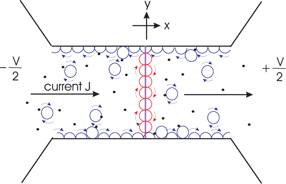
Let us consider a 2D dimensional electron system in the presence of a lateral barrier subject to an external magnetic field applied perpendicular to its plane as is shown in Fig.1.
In this paper electron dynamics and kinetics are considered in the semiclassical approximation that is where is the cyclotron frequency and is the Fermi energy. It is also assumed that the electron free path length where is the Larmour radius and is the Fermi momentum; the width of the sample and hence the contribution of the conventional edge states (which are localized at the external boundaries) to the sample conductance is negligible. The -axis is parallel to the current flowing along the biased sample while the -axis is along the lateral barrier.
II.1 Dynamics of quasi-particles skipping along the lateral junction under magnetic field.
As is seen in Fig.1 electrons are in three qualitatively different states: a) there are electrons in the Landau states moving along closed orbits, b) those in the conventional edge states skipping along the external boundaries of the sample, and c) electrons in peculiar field-dependent quasi-particle states highly localized around the lateral barrier. The quantum interference between the left and right edge states results in peculiar one-dimensional spectrum arises.
As shown in AppendixA, at low transparency of the barrier the dispersion equation which determines the energy of quasi-particles skipping along the barrier is
| (1) |
where and while is the conserving projection of the generalized electron momentum on the direction of the lateral barrier while
| (2) |
Here . As one easily sees does not depend on .
One sees from Eq.(1) that at there are a large number of crossing points of the spectra of the left and right independent edge states (see Appendix ). At final barrier transparency the degeneracy is lifted that opens gaps in the quasi-particle spectrum (see Fig.2).

As follows from Eq.(1) degeneration takes place at if two equations are satisfied:
| (3) |
Hence positions of the degeneration points in the plane are determined by the conditions: and where are integer. Summing and subtracting them with the use of Eq.(2) one gets
| (4) |
where and .
Therefore, the degeneration points are in line with discrete Landau levels being situated in discrete points inside the each Landau level and hence their positions may be uniquely classified with two discrete indexes as .
One easily sees that the distances between neighboring points are
| (5) |
Therefore, if is a slow varying function of the momentum on the scale one may changes the summation with respect to to the integration as follows:
| (6) |
Summing up, the spectrum of electrons skipping along the junction is an alternating sequence of narrow energy bands (the widths of which are ) and energy gaps (see Ref.[8, 9, 10]), the latter lining discrete Landau levels (n is the Landau number).

II.2 Current flowing along dirty sample and perpendicular to lateral junction under magnetic field.
As in the case of the magnetic breakdown phenomenon, dynamic and kinetic properties of quasi-particles skipping along the junction under magnetic field are of the fundamentally quantum mechanical nature due to the quantum interference of their wave functions with semiclassically large phases. Thus, in order to analyze the transport properties of the quasi-particles in the presence of impurities it is convenient to start with the equation for the density matrix in the -approximation:
| (7) |
Here, is the Hamiltonian of the system under consideration in the absence of the bias voltage , is the Fermi distribution function, is the electron scattering time.
In this paper we assume that the barrier transparency is so low that the main drop of the voltage applied to the sample takes place on the lateral barrier, that is it may be written as
| (8) |
where is the voltage drop on the barrier and is the unit step function.
Writing the density matrix in the form and linearizing Eq.(7) with respect to the bias potential one gets
| (9) |
In terms of the density matrix the the current density at a point is written as follows:
| (10) |
where is the operator of the quasi-particle velocity.
Taking matrix elements of equation Eq.(9) with respect to the proper functions of the Hamiltonian written in the Dirac notations
| (11) |
one finds the density matrix. Inserting the found solution in Eq.(10) one obtains the current flowing perpendicular to the barrier as follows:
| (12) |
where and is the electron-impurity relaxation frequency. The equation is written under assumption that . Matrix elements of the applied voltage and the velocity operator are presented in Appendix (see Eqs.(28,31)).
Such a peculiar dynamics as is described in Subsection II.1 manifests itself in the resonant properties of the matrix elements in Eq.(12) that is especially pronounced at . Consider, e.g., , Eq.(28). At the wave functions in Eq.(27) are orthogonal edge state functions and hence at . Therefore, one has exclusively due to a final barrier transparency. Using Eq.(1) one easily finds that far from the degenerate points while in the vicinity of them the resonance tunnelling takes place and and hence the main contribution to the integral in Eq.(12) is from in the vicinity of the degenerate points (see Eq.(4).
Therefore, when calculating the current Eq.(12) one may use Eqs.(29,33) and get it as follows:
| (13) |
where and while and is the x-coordinate of the electron which is defined by the classical Hamilton equation Eq.(32).
Expanding the integrand in the vicinities of degeneration points (where the resonant tunnelling takes place) with the use of Eq.(26) one re-writes the current, Eq.(13), as follows:
| (14) |
Here the summation is over all the degeneration points; is the electron-impurity relaxation time, and are the velocities of the left (1) and right (2) edge states at while and are the times of electron motion between points and along the left and right classical orbits shown in Fig.3, respectively:
| (15) |
All the above-mentioned quantities are taken at .
The first resonant term of the integrand is due to the resonant transmission of electrons between left and right edge states skipping along the lateral junction: at the degenerate points the widths of the left and right wells (which are created by the magnetic field) are of such values that the electron energies in them (at ) coincide causing resonant transmissions between the wells (see Eq.26 and the text below it).
For the case that the temperature satisfies the inequality one may expand the Fermi distribution functions with respect to and obtain the current as follows:
| (16) | |||||
where is the Drude conductivity , is the electron density. While writing this equation the summation with respect to was changed to integration according to Eq.(6).
As one sees from Eq.(16), at the current oscillates with a giant amplitude under a change of the magnetic field or the gate voltage (see Fig.4).
If the summation with respect to may be changed to integration, , and the current oscillations are smoothed out and the current becomes of the conventional form.

In conclusion, it is shown that kinetic properties of a dirty 2DEG system with lateral junction under magnetic field is extremely sensitive to actions of external fields. In particular, even a rather weak variation of the magnetic filed or the gate voltage causes giant oscillations of the charge current flowing perpendicular to the junction. The theoretical analysis based on quantum resonance tunnelling of quasi-particles skipping along the junction is in a good agreement with experimental data: the period of the conductance oscillations, the position and the value of the conductance maxima correspond to the observations presented in Rwf..
Appendix A Wave functions and dispersion equation for quasi-particles skipping along lateral junction.
Quantum dynamics of electrons with a lateral junction under magnetic field is described by the wave function satisfying the two-dimensional Schrödinger equation:
| (17) | |||||
where the gauge is used for which the vector-potential ,
The semiclassical solutions of the above equation on the left and right sides of the junction ( and , respectively) are
| (18) |
where quantum numbers and are the band number and the conserving projection momentum, respectively while
| (19) |
Here are the turning points. The dependence of the constant factors , and the quasi-particle dispersion law are found by matching the above wave functions at the lateral barrier and their normalization as it is shown below.
In the vicinity of the junction , one may expand the phases of the wave functions Eq.(18) in and see that they are incoming and outgoing plane waves the constant factors at which and are
| (20) |
where
| (21) |
Changing variables in the integrals here one finds Eq.(2) of the main text.
The found plane waves undergo two-channel scattering at the junction and the constant factors at the outgoing functions are coupled with the incoming ones with a scattering unitary matrix which is written in the general case as follows:
| (22) |
where and are the probability amplitudes for the incoming electron to pass through and to be scattered back at the junction, respectively, .
Using Eqs.(20,22) one finds the set of equations that couples the constant factors in wave functions Eq.(18):
| (23) |
where . Equating the determinant of equation Eq.23 to zero and using the inequality one finds dispersion equation Eq.(1) of the main text.
Using equations Eq.(1) one easily finds the quasi-particle dispersion law in the vicinity of points of degeneration, , as follows:
| (24) |
where and while definitions of the velocities and times at degeneration points are given by Eq.(15).
Normalization of the wave function Eq.(18) to unity gives the second independent equation for constants :
| (25) |
where are times of electron motion along classical orbits 1 and 2.
For the case under considerations , using Eqs.(23,25) one finally finds
| (26) |
where functions are determined by Eq.(2).
Using Eq.(24) one easily finds at degeneracy point and hence that is a resonant tunnelling takes place at these points.
Appendix B Matrix elements of applied voltage and quasi-particle velocity.
In the vicinity of degeneration points one has and hence Eq.(27) may be written as follows:
| (29) |
2. Matrix elements of the quasi-particle velocity are
| (30) | |||||
Using the explicit form of the semiclassical wave functions Eq.(18) one finds the velocity matrix elements as follows
| (31) |
where is defined by the classical Hamilton equation:
| (32) |
while and are coordinates of semiclassical packets moving along the left and right sections of the closed orbit, respectively (see Fig.3). They are defined in such a way that their motion starts at the beginning of the corresponding section: e.g., for the motion along the closed orbit in Fig.3 , and , .
Using inequality , near degeneration points one may write Eq.(31) in the form:
| (33) |
References
- [1] V. L. Berezinskii, Sov. Phys. JETP, 32, 493 (1971).
- [2] J. M. Kosterlitz and D. J. Thouless, Journal of Physics C: Solid State Physics, 6, 1181 (1973).
- [3] Th. Heinzel, Mesoscopic Electronics in Solid State Nanostructures, Wiley-VCH (2003).
- [4] W. Zwerger, Theory of Coherent Transport in Th. Dittrich, G-L. Ingold, G. Schön, P. Hänggi, B. Kramer, and W. Zwerger, Quantum Transport and Dissipation, Wiley-VCH (1998).
- [5] B. Kramer, 1998 Quantization of Transport, in Th. Dittrich, G-L. Ingold, G. Schön, P. Hänggi, B. Kramer, and W. Zwerger, Quantum Transport and Dissipation, Wiley-VCH (1998).
- [6] M. H. Devoret , J. M. Martinis, and J. Clarke, 1985 Phys. Rev. Lett. 55 (1908); J. M. Martinis, M. H. Devoret, and J. Clarke Phys. Rev. B 35, 4682 (1987).
- [7] C. W. J. Beenakker and H. van Houten, Solid State Physics, 441 (1991).
- [8] W. Kang, H.L. Stormer, L.N. Pfeifer, K.W. Baldwin, and K.W. West, Letters to Nature, 403, 59 (2000).
- [9] A.M. Kadigrobov, M.V. Fistul, and K.B. Efetov, Phys. Rev. B 73, 235313 (2006).
- [10] A.M. Kadigrobov, arXiv:1609.06648, to be published in Low Temperature Physics 43, No 1 (2017).
- [11] Morrel H. Cohen and L.M. Falikov, Pfys. Rev. Lett. 6, 231 (231).
- [12] M.I. Kaganov and A.A. Slutskin, Physics Reports 98, 189 (1983).
- [13] A.A. Slutskin and A.M. Kadigrobov, Soviet Physics - Solid State, 9, 138 (1967).
- [14] A.A. Slutskin, Sov. Phys. JETP Lett. 26, 474 (1968).
- [15] A.A. Slutskin and A.M. Kadigrobov, JETP Lett. 32, 338 (1980)
- [16] A.A. Slutskin and A.M. Kadigrobov, Physica B & C 108, 877 (1981).
- [17] Y.A. Kolesnichenko, V.G. Peschanski, Fizika Nizkikh Temperatur 10, 1141 (1984)
- [18] A.M. Kadigrobov and I.V. Koshkin, Sov. J. Low Temp. Phys. 12, 249 (1986).
- [19] A.M. Kadigrobov and M.V. Fistul, J. Phys.: Condens. Matter 28, 255301 (2016).