跳到论文正文
W Papers独立论文阅读器 arXiv:1704.07868 论文正文 计算阅读时间 · 0%
引用这篇论文根据当前论文元数据生成,正式投稿前建议核对。


License: arXiv.org perpetual non-exclusive license
arXiv:1704.07868v3 [stat.ME] 26 Jun 2018

New robust statistical procedures for polytomous logistic regression models

Castilla    E.; Ghosh Affiliation: Complutense University of Madrid, 28040 Madrid, Spain    A; Martín Affiliation: Indian Statistical Institute, Kolkata, India    N Affiliation: Complutense University of Madrid, 28040 Madrid, Spain    Pardo    L Affiliation: Complutense University of Madrid, 28040 Madrid, Spain
August 24, 2026
Abstract

This paper derives a new family of estimators, namely the minimum density power divergence estimators, as a robust generalization of the maximum likelihood estimator for the polytomous logistic regression model. Based on these estimators, a family of Wald-type test statistics for linear hypotheses is introduced. Robustness properties of both the proposed estimators and the test statistics are theoretically studied through the classical influence function analysis. Appropriate real life examples are presented to justify the requirement of suitable robust statistical procedures in place of the likelihood based inference for the polytomous logistic regression model. The validity of the theoretical results established in the paper are further confirmed empirically through suitable simulation studies. Finally, an approach for the data-driven selection of the robustness tuning parameter is proposed with empirical justifications.

MSC: 62F35, 62F05

Keywords: Influence function; Minimum density power divergence estimators; Polytomous logistic regression; Robustness; Wald-type test statistics.

1 Introduction

The polytomous logistic regression model (PLRM) is widely used in health and life sciences for analyzing nominal qualitative response variables (e.g., Daniels and Gatsonis, 1997; Blizzard and Hosmer, 2007; Bull, Lewinger and Lee, 2007; Dreassi, 2007; Biesheuvel et al., 2008; Bertens et al., 2015; Dey, Raheem and Lu, 2016; Ke, Fu and Zhang, 2016, and the references therein). Such examples occur frequently in medical studies where disease symptoms may be classified as absent, mild or severe, the invasiveness of a tumor may be classified as in situ, locally invasive, or metastatic, etc. The qualitative response models specify the multinomial distribution for such a response variable with individual category probabilities being modeled as a function of suitable explanatory variables. One such popular model is the PLRM, where the logit function is used to link the category probabilities with the explanatory variables.

Mathematically, let us assume that the nominal outcome variable Y~\tilde{Y} has d+1d+1 categories C1,…,Cd+1C_{1},...,C_{d+1} and we observe Y~\tilde{Y} together with kk explanatory variables with given values xhx_{h}, h=1,…,kh=1,...,k. In addition, assume that 𝜷jT=(β0​j,β1​j,…,βk​j),\boldsymbol{\beta}_{j}^{T}=\left(\beta_{0j},\beta_{1j},...,\beta_{kj}\right), j=1,…,dj=1,...,d, is a vector of unknown parameters and 𝜷d+1\boldsymbol{\beta}_{d+1} is a (k+1)(k+1)-dimensional vector of zeros; i.e., the last category Cd+1C_{d+1} has been chosen as the baseline category. Since the full parameter vector 𝜷T=(𝜷1T,…,𝜷dT)\boldsymbol{\beta}^{T}=(\boldsymbol{\beta}_{1}^{T},...,\boldsymbol{\beta}_{d}^{T}) is ν\nu-dimensional with ν=d⁡(k+1)\nu=d(k+1), the parameter space is Θ=ℝd⁡(k+1)\Theta=\mathbb{R}^{d(k+1)}. Let πj​(𝒙,𝜷)=P⁡(Y~∈Cj∣𝒙,𝜷)\pi_{j}\left(\boldsymbol{x},\boldsymbol{\beta}\right)=P(\tilde{Y}\in C_{j}\mid\boldsymbol{x},\boldsymbol{\beta}{)} denote the probability that Y~\tilde{Y} belongs to the category CjC_{j} for j=1,…,d+1,j=1,...,d+1, when the vector of explanatory variable takes the value 𝒙T=(x0,x1,…,xk)\boldsymbol{x}^{T}=(x_{0},x_{1},\ldots,x_{k}), with x0=1x_{0}=1 being associated with the intercept β0​j{\beta}_{0j}. Then, the PLRM is given by

πj(𝒙,𝜷)=exp(𝒙T𝜷j)/{1+∑h=1dexp(𝒙T𝜷h)}, j=1,…,d+1.\pi_{j}\left(\boldsymbol{x},\boldsymbol{\beta}\right)=\exp(\boldsymbol{x}^{T}\boldsymbol{\beta}_{j})\left/\left\{1+\sum_{h=1}^{d}\exp(\boldsymbol{x}^{T}\boldsymbol{\beta}_{h})\right\},\right.\text{ }j=1,...,d+1. (1)

Now assume that we have observed the data on NN individuals having responses 𝒚~i\tilde{\boldsymbol{y}}_{i} with associated covariate values (including intercept) 𝒙i∈ℝk+1\boldsymbol{x}_{i}\in\mathbb{R}^{k+1}, i=1,…,Ni=1,...,N, respectively. For each individual, let us introduce the corresponding tabulated response 𝒚i=(yi​1,…,yi,d+1)T\boldsymbol{y}_{i}=\left(y_{i1},...,y_{i,d+1}\right)^{T} with yi​ry_{ir} =1=1 and yi​s=0y_{is}=0 for s∈{1,…,d+1}−{r}s\in\left\{1,...,d+1\right\}-\left\{r\right\} if 𝒚~i∈Cr\tilde{\boldsymbol{y}}_{i}\in C_{r}. The most common estimator of 𝜷\boldsymbol{\beta} under the PLRM is the maximum likelihood estimator (MLE), which is obtained by maximizing the loglikelihood function, log⁡ℒ⁡(𝜷)≡∑i=1N∑j=1d+1yi​j​log⁡πj​(𝒙i,𝜷)\log\mathcal{L}\left(\boldsymbol{\beta}\right)\equiv\sum_{i=1}^{N}\sum_{j=1}^{d+1}y_{ij}\log\pi_{j}\left(\boldsymbol{x}_{i},\boldsymbol{\beta}\right). One can then develop all the subsequent inference procedures based on the MLE 𝜷^\widehat{\boldsymbol{\beta}} of 𝜷\boldsymbol{\beta}. Although the MLE has optimal asymptotic properties in relation to the efficiency for most cases, its serious lack of robustness against the outlying observations is also a well-known problem. However, in any practical dataset it is quite natural to have outlying observations which can lead to incorrect inference for the likelihood based approach and can be very dangerous specially in applications like medical sciences. The above formulation of the PLRM is not exclusive only for distinct covariate values; it can also be applied, with the same notation, if multiple responses are observed for the same covariate values. Let us begin with the following motivating example.

Example 1 (Mammography experience data)

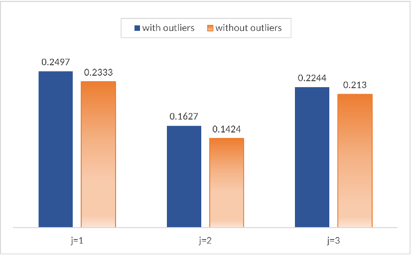
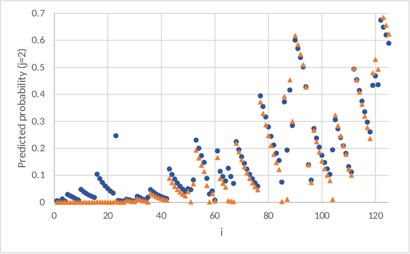
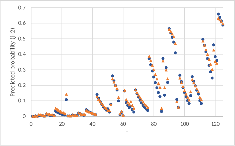
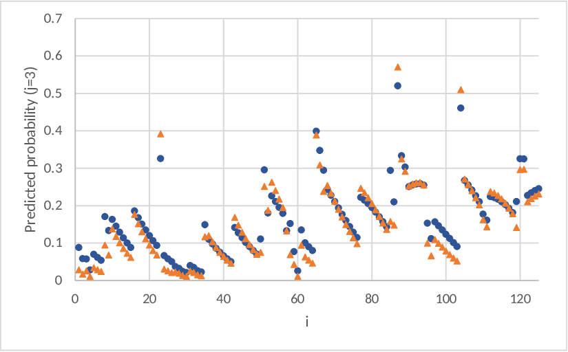
The mammography experience data, which assess factors associated with women’s knowledge, attitude and behavior towards mammography, was introduced in Hosmer and Lemeshow (2000); it is a subset of the original study by the University of Massachusetts Medical School and recently studied by Martín (2015). It involves N=412N=412 individuals, k=8k=8 explanatory variables and a nominal response with d+1=3d+1=3 categories (studied in detail in Section 5). Here, all individuals do not have distinct covariate values so that their plots (e.g., Figure 1) only distinguish 125125 indices in its x-axis, which corresponds to the grouped observations for 125 distinct covariates values available in the data. Following Martín (2015), the grouped observations associated with seven such distinct indices can be considered as outliers. A “good” robust statistical inference procedure should not get highly affected by the presence of the outliers. So, we compute the MLE of 𝛃\boldsymbol{\beta} under the PLRM for the full dataset and also for the outliers deleted dataset and plot the corresponding (estimated) category probabilities for each available distinct covariate values. The left panel of Figure 1 presents these category probabilities for the second category, which clearly indicates the significant variation of the MLE in the presence or absence of the outliers. In addition, the mean deviations of the estimated probabilities with respect to the relative frequencies, shown in Figure 1 (right), are always seen to be lower for the outlier deleted estimators. This introductory example clearly illustrates the non-robust nature of the MLE and motivates us to look for a robust inference procedure that will generate correct results with high efficiency even without removing the outlying observations. □\square
Refer to caption
Refer to caption
Figure 1: MLE based estimates of (a) the response probabilities in category j=2j=2 (left) and (b) the expected mean deviations of the estimated probabilities with respect to the corresponding relative frequencies for each category j=1,2,3j=1,2,3 (right) in the Mammography experience data

The term “outlier”needs a clarification when referring Martín (2015). In logistic regression diagnostics, the Cook’s distance is a tool for identifying influential observations associated with specific explanatory variables. In the current paper, the term “outlier”matches this notion of “influency ”but not directly the term “outlying for having a large value of the residual”, as in Martín (2015).

There exist some alternative estimation procedures for the PLRM other than the MLE, although they are used less often in practice; these include the estimators proposed by Begg and Gray (1984) and its modification by Rom and Cohen (1995). The generalized method of moments (GMM) has also been considered (Hayashi, 2000) which has been shown to be consistent and fully efficient under suitable conditions. Gupta et al. (2006) considered the PLRM with only categorical covariates and discussed the family of the minimum phi-divergence estimators (Mϕ\phiEs) that contains the MLE as a particular case. The Mϕ\phiEs are BAN estimators and have high efficiency for moderate and small sample sizes. However, the important issue of robustness against outliers was ignored in all these cited references. Ronchetti and Trojani (2001) pointed out the non-robustness of the GMM estimators. Recently, Wang (2014) gave a robust modification of the GMM estimator, whereas earlier Victoria-Feser and Ronchetti (1997) had presented a robust estimator for grouped data with categorical covariates only.

In this paper, we present an alternative simple robust generalization of the MLE for the general PLRM (1) by using the density power divergence (DPD) measure of Basu et al. (1998). The DPD based inference has become very popular in recent time specially because of its strong robustness properties against outliers; see, e.g., Basu et al. (2016, 2017a,b), Ghosh et al. (2016), among others. In this paper, we first develop the estimator of 𝜷\boldsymbol{\beta} in the PLRM by minimizing a suitably defined DPD measure and derive its asymptotic distribution in Section 2. In Section 3 the problem of testing linear hypotheses in the PLRM is considered using the newly proposed estimators. The robustness of both the proposed estimator and the test of hypothesis are studied theoretically through the influence function analysis in Section 4. Section 5 presents some real data examples and Section 6 is devoted to a simulation study. A method for the data-driven selection of the robustness tuning parameter is described in Section 7. The paper ends with brief concluding remarks in Section 8. Proofs of the results and further technical details are given in the online supplementary material.

2 Minimum density power divergence estimator for the PLRM

The MLE 𝜷^\widehat{\boldsymbol{\beta}} of the parameter 𝜷\boldsymbol{\beta} under the PLRM in (1) can be equivalently defined as the minimizer of the Kullback-Leibler divergence (KLD) between the probability vectors 𝒑^=1N​(y11,…,y1,d+1,y21,…CLOSE,\widehat{\boldsymbol{p}}=\frac{1}{N}(y_{11},...,y_{1,d+1},y_{21},..., OPENy2,d+1,…,yN​1,…,yN,d+1)Ty_{2,d+1},...,y_{N1},...,y_{N,d+1})^{T} and 𝒑⁡(𝜷)=1N​(𝝅1​(𝜷)T,…,𝝅N​(𝜷)T)T\boldsymbol{p}(\boldsymbol{\beta})=\frac{1}{N}(\boldsymbol{\pi}_{1}(\boldsymbol{\beta})^{T},...,\boldsymbol{\pi}_{N}(\boldsymbol{\beta})^{T})^{T}, where 𝝅i​(𝜷)T=(πi​1​(𝜷),…,πi,d+1​(𝜷))\boldsymbol{\pi}_{i}\left(\boldsymbol{\beta}\right)^{T}=(\pi_{i1}(\boldsymbol{\beta}),\ldots,\pi_{i,d+1}(\boldsymbol{\beta})), with πi​j​(𝜷)=πj​(𝒙i,𝜷)\pi_{ij}(\boldsymbol{\beta})=\pi_{j}\left(\boldsymbol{x}_{i},\boldsymbol{\beta}\right). This follows from the expression of the KLD between 𝒑^\widehat{\boldsymbol{p}} and 𝒑⁡(𝜷)\boldsymbol{p}\left(\boldsymbol{\beta}\right) given by

DK​L​(𝒑^,𝒑⁡(𝜷))=∑i=1N∑j=1d+1yi​jN​log⁡yi​jπi​j​(𝜷)=c−1N​∑i=1N∑j=1d+1yi​j​log⁡πi​j​(𝜷),D_{KL}\left(\widehat{\boldsymbol{p}},\boldsymbol{p}\left(\boldsymbol{\beta}\right)\right)=\sum_{i=1}^{N}\sum_{j=1}^{d+1}\dfrac{y_{ij}}{N}\log\frac{y_{ij}}{\pi_{ij}\left(\boldsymbol{\beta}\right)}=c-\dfrac{1}{N}\sum_{i=1}^{N}\sum_{j=1}^{d+1}y_{ij}\log\pi_{ij}\left(\boldsymbol{\beta}\right), (2)

where cc does not depend on 𝜷\boldsymbol{\beta} and hence 𝜷^=arg⁡min𝜷∈𝚯​DK​L​(𝒑^,𝒑⁡(𝜷))\widehat{\boldsymbol{\beta}}=\arg\min_{\boldsymbol{\beta}\mathbf{\in\Theta}}D_{KL}\left(\widehat{\boldsymbol{p}},\boldsymbol{p}\left(\boldsymbol{\beta}\right)\right).

The KLD is a particular case of the general DPD measure Dλ​(⋅,⋅)D_{\lambda}(\cdot,\cdot) between 𝒑^\widehat{\boldsymbol{p}} and 𝒑⁡(𝜷)\boldsymbol{p}\left(\boldsymbol{\beta}\right)

Dλ​(𝒑^,𝒑⁡(𝜷))=1Nλ+1​∑i=1N{∑j=1d+1πi​jλ+1​(𝜷)−λ+1λ​∑j=1d+1yi​l​πi​jλ​(𝜷)+1λ}.D_{\lambda}\left(\widehat{\boldsymbol{p}},\boldsymbol{p}\left(\boldsymbol{\beta}\right)\right)=\frac{1}{N^{\lambda+1}}\sum\limits_{i=1}^{N}\left\{\sum\limits_{j=1}^{d+1}\pi_{ij}^{\lambda+1}\left(\boldsymbol{\beta}\right)-\frac{\lambda+1}{\lambda}\sum\limits_{j=1}^{d+1}y_{il}\pi_{ij}^{\lambda}\left(\boldsymbol{\beta}\right)+\frac{1}{\lambda}\right\}.

Since the term 1λ\frac{1}{\lambda} does not have any role in the minimization of Dλ​(𝒑^,𝒑​(𝜷))D_{\lambda}\left(\widehat{\boldsymbol{p}},\boldsymbol{p}\left(\boldsymbol{\beta}\right)\right) with respect to 𝜷\boldsymbol{\beta}, it is sufficient to consider dλ​(𝒚i,𝝅i​(𝜷))=∑j=1d+1{πi​j​(𝜷)−λ+1λ​yi​j}​πi​j​(𝜷)λd_{\lambda}\left(\boldsymbol{y}_{i},\boldsymbol{\pi}_{i}(\boldsymbol{\beta})\right)=\sum_{j=1}^{d+1}\left\{\pi_{ij}\left(\boldsymbol{\beta}\right)-\tfrac{\lambda+1}{\lambda}y_{ij}\right\}\pi_{ij}\left(\boldsymbol{\beta}\right)^{\lambda}, and minimize

dλ​(𝒑^,𝒑⁡(𝜷))=1Nλ+1​∑i=1Ndλ​(𝒚i,𝝅i​(𝜷)).d_{\lambda}\left(\widehat{\boldsymbol{p}},\boldsymbol{p}\left(\boldsymbol{\beta}\right)\right)=\frac{1}{N^{\lambda+1}}\sum\limits_{i=1}^{N}d_{\lambda}\left(\boldsymbol{y}_{i},\boldsymbol{\pi}_{i}(\boldsymbol{\beta})\right). (3)
Definition 2

The minimum DPD estimator (MDPDE) of 𝛃\boldsymbol{\beta} with tuning parameter λ\lambda in the PLRM (1) is given by 𝛃^λ=arg⁡min𝛃∈Θ​dλ​(𝐩^,𝐩⁡(𝛃))\widehat{\boldsymbol{\beta}}_{\lambda}=\displaystyle\arg\min_{\boldsymbol{\beta\in}\Theta}d_{\lambda}\left(\widehat{\boldsymbol{p}},\boldsymbol{p}\left(\boldsymbol{\beta}\right)\right), where dλ​(𝐩^,𝐩​(𝛃))d_{\lambda}\left(\widehat{\boldsymbol{p}},\boldsymbol{p}\left(\boldsymbol{\beta}\right)\right) is given in (3).

The DPD at λ=0\lambda=0 is defined by the limit of the expression in (3) as λ→0\lambda\rightarrow 0, which coincides with the KLD (2) up to an additive constant. Therefore, the MDPDE at λ=0\lambda=0 is nothing but the MLE. See Appendix for the detailed procedure to obtain the MDPDE.

Note that the random variables 𝒀i\boldsymbol{Y}_{i} associated with the tabulated response 𝒚i\boldsymbol{y}_{i}, given the covariate value 𝒙i\boldsymbol{x}_{i} under the PLRM, are independent but non-homogeneous. So, we can apply the general theory from Ghosh and Basu (2013) to study the properties of the MDPDE under the PLRM. In fact, the minimization of the intuitive objective function (3) here is equivalent to the minimization of the average DPD measure between the observed data and the model probability mass functions over each distributions (indexed by ii), which is proposed in Ghosh and Basu (2013) for the general non-homogeneous set-up. Hence, based on their general theory, we obtain the asymptotic properties of our MDPDE under the PLRM which is presented in the following theorem.

Theorem 3

Consider the PLRM (1) with the true parameter value being 𝛃0\boldsymbol{\beta}_{0}. Under Assumptions (A1)–(A7) of Ghosh and Basu (2013), there exists a consistent MDPDE 𝛃^λ\widehat{\boldsymbol{\beta}}_{\lambda} of 𝛃\boldsymbol{\beta} and N​(𝛃^λ−𝛃0)​→N→∞ℒ​𝒩​(𝟎d⁡(k+1),𝐉λ−1​(𝛃0)​𝐕λ​(𝛃0)​𝐉λ−1​(𝛃0))\sqrt{N}(\widehat{\boldsymbol{\beta}}_{\lambda}-\boldsymbol{\beta}_{0})\overset{\mathcal{L}}{\underset{N\rightarrow\infty}{\rightarrow}}\mathcal{N}\left(\boldsymbol{0}_{d(k+1)},\boldsymbol{J}_{\lambda}^{-1}\left(\boldsymbol{\beta}_{0}\right)\boldsymbol{V}_{\lambda}\left(\boldsymbol{\beta}_{0}\right)\boldsymbol{J}_{\lambda}^{-1}\left(\boldsymbol{\beta}_{0}\right)\right), where 𝐉λ​(𝛃)=limN→∞𝚿N,λ​(𝛃)\boldsymbol{J}_{\lambda}\left(\boldsymbol{\beta}\right)=\lim\limits_{N\rightarrow\infty}\boldsymbol{\Psi}_{N,\lambda}\left(\boldsymbol{\beta}\right) and 𝐕λ​(𝛃)=limN→∞𝛀N,λ​(𝛃)\boldsymbol{V}_{\lambda}\left(\boldsymbol{\beta}\right)=\lim\limits_{N\rightarrow\infty}\boldsymbol{\Omega}_{N,\lambda}\left(\boldsymbol{\beta}\right) with

𝚿N,λ​(𝜷)=1N​∑i=1N𝚫⁡(𝝅i∗​(𝜷))​diagλ−1​{𝝅i∗​(𝜷)}​𝚫​(𝝅i∗​(𝜷))⊗𝒙i​𝒙iT,\boldsymbol{\Psi}_{N,\lambda}\left(\boldsymbol{\beta}\right)=\frac{1}{N}\sum\limits_{i=1}^{N}\boldsymbol{\Delta}(\boldsymbol{\pi}_{i}^{\ast}\left(\boldsymbol{\beta}\right))\mathrm{diag}^{\lambda-1}\{\boldsymbol{\pi}_{i}^{\ast}\left(\boldsymbol{\beta}\right)\}\boldsymbol{\Delta}(\boldsymbol{\pi}_{i}^{\ast}\left(\boldsymbol{\beta}\right))\otimes\boldsymbol{x}_{i}\boldsymbol{x}_{i}^{T}, (4)
𝛀N,λ​(𝜷)=1N​∑i=1N𝚫⁡(𝝅i∗​(𝜷))​diagλ−1​{𝝅i∗​(𝜷)}​𝚫​(𝝅i∗​(𝜷))​diagλ−1​{𝝅i∗​(𝜷)}​𝚫​(𝝅i∗​(𝜷))⊗𝒙i​𝒙iT.\boldsymbol{\Omega}_{N,\lambda}\left(\boldsymbol{\beta}\right)=\frac{1}{N}\sum\limits_{i=1}^{N}\boldsymbol{\Delta}(\boldsymbol{\pi}_{i}^{\ast}\left(\boldsymbol{\beta}\right))\mathrm{diag}^{\lambda-1}\{\boldsymbol{\pi}_{i}^{\ast}\left(\boldsymbol{\beta}\right)\}\boldsymbol{\Delta}(\boldsymbol{\pi}_{i}^{\ast}\left(\boldsymbol{\beta}\right))\mathrm{diag}^{\lambda-1}\{\boldsymbol{\pi}_{i}^{\ast}\left(\boldsymbol{\beta}\right)\}\boldsymbol{\Delta}(\boldsymbol{\pi}_{i}^{\ast}\left(\boldsymbol{\beta}\right))\otimes\boldsymbol{x}_{i}\boldsymbol{x}_{i}^{T}. (5)

Here, 𝚫⁡(𝐩)=diag⁡(𝐩)−𝐩​𝐩T\boldsymbol{\Delta}(\boldsymbol{p})=\mathrm{diag}(\boldsymbol{p})-\boldsymbol{pp}^{T}, the vector with superscript ∗\ast denotes its subvector with the last element removed and the vector with any other superscript takes the corresponding power for all its components.

3 Wald-type test statistics for testing linear hypotheses

Most testing problems for 𝜷\boldsymbol{\beta} in the PLRM belong to the class of linear hypotheses given by

H0:𝑳T​𝜷=𝒉​ against ​H1:𝑳T​𝜷≠𝒉,H_{0}:\boldsymbol{L}^{T}\boldsymbol{\beta}=\boldsymbol{h}\text{ against }H_{1}:\boldsymbol{L}^{T}\boldsymbol{\beta}\neq\boldsymbol{h}, (6)

where 𝑳\boldsymbol{L} is d⁡(k+1)×rd(k+1)\times r full rank matrix with r≤d⁡(k+1)r\leq d(k+1) and 𝒉\boldsymbol{h} an rr-vector. Two important particular cases are the testing problems for H0:𝜷=𝜷0H_{0}:\boldsymbol{\beta}=\boldsymbol{\beta}_{0} or H0:𝜷(s)=𝟎H_{0}:\boldsymbol{\beta}_{(s)}=\boldsymbol{0} against their respective omnibus alternatives, where 𝜷(s)\boldsymbol{\beta}_{(s)} is a subvector of 𝜷\boldsymbol{\beta}.

Definition 4

Let 𝛃^λ\widehat{\boldsymbol{\beta}}_{\lambda} be the MDPDE of 𝛃\boldsymbol{\beta} in the PLRM (1) and denote 𝐌N,λ​(𝛃^λ)=\boldsymbol{M}_{N,\lambda}(\widehat{\boldsymbol{\beta}}_{\lambda})= 𝚿N,λ−1​(𝛃^λ)​𝛀N,λ​(𝛃^λ)\boldsymbol{\Psi}_{N,\lambda}^{-1}(\widehat{\boldsymbol{\beta}}_{\lambda})\boldsymbol{\Omega}_{N,\lambda}(\widehat{\boldsymbol{\beta}}_{\lambda}) 𝚿N,λ−1​(𝛃^λ)\boldsymbol{\Psi}_{N,\lambda}^{-1}(\widehat{\boldsymbol{\beta}}_{\lambda}). Then, the family of Wald-type test statistics for testing the null hypothesis given in (6) is defined as

WN​(𝜷^λ)=N​(𝑳T​𝜷^λ−𝒉)T​{𝑳T​𝑴N,λ​(𝜷^λ)​𝑳}−1​(𝑳T​𝜷^λ−𝒉).W_{N}(\widehat{\boldsymbol{\beta}}_{\lambda})=N(\boldsymbol{L}^{T}\widehat{\boldsymbol{\beta}}_{\lambda}-\boldsymbol{h})^{T}\left\{\boldsymbol{L}^{T}\boldsymbol{M}_{N,\lambda}(\widehat{\boldsymbol{\beta}}_{\lambda})\boldsymbol{L}\right\}^{-1}(\boldsymbol{L}^{T}\widehat{\boldsymbol{\beta}}_{\lambda}-\boldsymbol{h}). (7)

In particular, since 𝜷^λ=0=𝜷^\widehat{\boldsymbol{\beta}}_{\lambda=0}=\widehat{\boldsymbol{\beta}}, the MLE of 𝜷\boldsymbol{\beta}, and 𝑴N,λ=0​(β^)=𝚿N,λ=0−1​(𝜷^)\boldsymbol{M}_{N,\lambda=0}(\widehat{\beta})=\boldsymbol{\Psi}_{N,\lambda=0}^{-1}(\widehat{\boldsymbol{\beta}}) with

𝚿N,λ=0​(𝜷)=𝛀N,λ=0​(𝜷)=1N​∑i=1N𝚫⁡(𝝅i∗​(𝜷))⊗𝒙i​𝒙iT,\boldsymbol{\Psi}_{N,\lambda=0}\left(\boldsymbol{\beta}\right)=\boldsymbol{\Omega}_{N,\lambda=0}\left(\boldsymbol{\beta}\right)=\frac{1}{N}\sum\limits_{i=1}^{N}\boldsymbol{\Delta}(\boldsymbol{\pi}_{i}^{\ast}\left(\boldsymbol{\beta}\right))\otimes\boldsymbol{x}_{i}\boldsymbol{x}_{i}^{T},

being the Fisher information matrix, WN​(𝜷^λ=0)W_{N}(\widehat{\boldsymbol{\beta}}_{\lambda=0}) becomes the classical Wald test statistic.

Theorem 5

The asymptotic distribution of the Wald-type test statistics, WN​(𝛃^λ)W_{N}(\widehat{\boldsymbol{\beta}}_{\lambda}), under the null hypothesis in (6), is a chi-square distribution (χr2\chi_{r}^{2}) with rr degrees of freedom.

Based on Theorem 5, the null hypothesis in (6) will be rejected if WN​(𝜷^λ)>χr,α2W_{N}(\widehat{\boldsymbol{\beta}}_{\lambda})>\chi_{r,\alpha}^{2}, the upper α\alpha-th quantile of χr2\chi_{r}^{2}. See Appendix for some results about its power function.

4 Robustness Properties

We first study the robustness of the proposed MDPDE of 𝜷\boldsymbol{\beta} under the PLRM (1) through the influence function analysis. For any estimator defined in terms of a statistical functional 𝑼⁡(G)\boldsymbol{U}(G) in the set-up of independent and identically distributed (IID) data from the true distribution function GG, its influence function is defined as ℐ​ℱ​(𝒕,𝑼,G)=limϵ↓0𝑼⁡(Gϵ)−𝑼⁡(G)ϵ=∂𝑼⁡(Gϵ)∂ϵ|ϵ=0\mathcal{IF}\left(\boldsymbol{t},\boldsymbol{U},G\right)=\lim\limits_{\epsilon\downarrow 0}\frac{\boldsymbol{U}(G_{\epsilon})-\boldsymbol{U}(G)}{\epsilon}=\left.\frac{\partial\boldsymbol{U}(G_{\epsilon})}{\partial\epsilon}\right|_{\epsilon=0}, where Gϵ=(1−ϵ)G+ϵ∧𝒕G_{\epsilon}=(1-\epsilon)G+\epsilon\wedge_{\boldsymbol{t}} with ϵ\epsilon being the contamination proportion and ∧𝒕\wedge_{\boldsymbol{t}} being the degenerate distribution at the contamination point 𝒕\boldsymbol{t}. Thus, the (first order) influence function (IF), as a function of 𝒕\boldsymbol{t}, measures the standardized asymptotic bias (in its first order approximation) caused by the infinitesimal contamination at the point 𝒕\boldsymbol{t}. The maximum of this IF over 𝒕\boldsymbol{t} indicates the extent of bias due to contamination and hence lower its value, the more robust the estimator is.

For the present case of PLRM, given the value of 𝒙i\boldsymbol{x}_{i}, 𝒚i\boldsymbol{y}_{i}s are independent but not-identically distributed. The extended definition of IF for such non-homogeneous cases has been proposed in Huber (1983) and Ghosh and Basu (2013, 2016). Following the approach of the later, let GiG_{i} denote the true distribution function of 𝒚i\boldsymbol{y}_{i} having joint mass function gig_{i} and Fi​(𝜷)F_{i}\left(\boldsymbol{\beta}\right) denote the distribution function under the assumption of PLRM having joint mass function fi​(𝒚i,𝜷)=𝒚iT​𝝅i​(𝜷)=∑j=1d+1yi​j​πi​j​(𝜷)f_{i}(\boldsymbol{y}_{i},\boldsymbol{\beta})=\boldsymbol{y}_{i}^{T}\boldsymbol{\pi}_{i}\left(\boldsymbol{\beta}\right)=\sum_{j=1}^{d+1}y_{ij}\pi_{ij}({\boldsymbol{\beta}}). Denote 𝑮=(G1,⋯,GN)T\boldsymbol{G}=(G_{1},\cdots,G_{N})^{T}, 𝑭⁡(𝜷)=(F1​(𝜷),⋯,FN​(𝜷))T\boldsymbol{F}(\boldsymbol{\beta})=\left(F_{1}(\boldsymbol{\beta}),\cdots,F_{N}(\boldsymbol{\beta})\right)^{T} and 𝒴={𝒆j,d+1}j=1d+1\mathcal{Y}=\{\boldsymbol{e}_{j,d+1}\}_{j=1}^{d+1}, where 𝒆j,d+1\boldsymbol{e}_{j,d+1} is the jj-th column of the identity matrix of order d+1d+1. Note that, 𝒴\mathcal{Y} is the sample space of the response variable 𝒀i\boldsymbol{Y}_{i}. Then, the statistical functional 𝑼λ​(𝑮)\boldsymbol{U}_{\lambda}(\boldsymbol{G}) corresponding to the proposed MDPDE, 𝜷^λ\widehat{\boldsymbol{\beta}}_{\lambda}, of 𝜷\boldsymbol{\beta} is defined as the minimizer of

H⁡(𝜷)=∑i=1N{∑𝒚i∈𝒴fiλ+1​(𝒚i,𝜷)−λ+1λ​∑𝒚i∈𝒴fiλ​(𝒚i,𝜷)​gi​(𝒚i)},H(\boldsymbol{\beta})=\sum\limits_{i=1}^{N}\left\{\sum_{\boldsymbol{y}_{i}\boldsymbol{\in}\mathcal{Y}}f_{i}^{\lambda+1}(\boldsymbol{y}_{i},\boldsymbol{\beta})-\frac{\lambda+1}{\lambda}\sum_{\boldsymbol{y}_{i}\boldsymbol{\in}\mathcal{Y}}f_{i}^{\lambda}(\boldsymbol{y}_{i},\boldsymbol{\beta})g_{i}(\boldsymbol{y}_{i})\right\},

whenever it exists. When the assumption of PLRM holds with true parameter 𝜷0\boldsymbol{\beta}_{0}, we have gi​(𝒚i)=fi​(𝒚i,𝜷0)g_{i}(\boldsymbol{y}_{i})=f_{i}(\boldsymbol{y}_{i},\boldsymbol{\beta}_{0}), and thus H⁡(𝜷)=Nλ+1​dλ​(𝒑⁡(𝜷0),𝒑⁡(𝜷))H(\boldsymbol{\beta})=N^{\lambda+1}d_{\lambda}\left(\boldsymbol{p}\left(\boldsymbol{\beta}_{0}\right),\boldsymbol{p}\left(\boldsymbol{\beta}\right)\right); this is minimized at 𝜷=𝜷0\boldsymbol{\beta}=\boldsymbol{\beta}_{0} implying the Fisher consistency of the MDPDE functional 𝑼λ​(𝑮)\boldsymbol{U}_{\lambda}(\boldsymbol{G}) at the PLRM. Note that, in such non-homogeneous settings, outliers can be either in any one or more index i∈{1,…,N}i\in\{1,...,N\} for gig_{i}. Following the general results from Ghosh and Basu (2013), one can derive the IF of the MDPDE at 𝑭⁡(𝜷0)\boldsymbol{F}({\boldsymbol{\beta}}_{0}) as given by

ℐ​ℱi0​(𝒕i0,𝑼λ,𝑭𝜷0)=𝚿N,λ−1​(𝜷0)​1N​(𝑰d,𝟎d)​𝚫​(𝝅i0​(𝜷)​diagλ−1​{𝝅i0∗​(𝜷0)}​{𝒕i0∗−𝝅∗​(𝜷0)}⊗𝒙i0CLOSE,\mathcal{IF}_{i_{0}}(\boldsymbol{t}_{i_{0}};\boldsymbol{U}_{\lambda},\boldsymbol{F}_{{\boldsymbol{\beta}}_{0}})=\boldsymbol{\Psi}_{N,\lambda}^{-1}({\boldsymbol{\beta}}_{0})\frac{1}{N}\left(\boldsymbol{I}_{d},\boldsymbol{0}_{d}\right)\boldsymbol{\Delta}(\boldsymbol{\pi}_{i_{0}}\left(\boldsymbol{\beta}\right)\mathrm{diag}^{\lambda-1}\{\boldsymbol{\pi}_{i_{0}}^{\ast}\left({\boldsymbol{\beta}}_{0}\right)\}\left\{\boldsymbol{t}_{i_{0}}^{\ast}-\boldsymbol{\pi}^{\ast}\left({\boldsymbol{\beta}}_{0}\right)\right\}\otimes\boldsymbol{x}_{i_{0}},

when there is contamination in only one specific index i0i_{0} at the point 𝒕i0∈𝒴\boldsymbol{t}_{i_{0}}\in\mathcal{Y} and

ℐ​ℱ​(𝒕¯,𝑼λ,𝑭⁡(𝜷0))=𝚿N,τ−1​(𝜷0)​1N​∑i=1N(𝑰d,𝟎d)​𝚫​(𝝅i​(𝜷)​diagλ−1​{𝝅i∗​(𝜷0)}​{𝒕i∗−𝝅∗​(𝜷0)}⊗𝒙iCLOSE,\mathcal{IF}(\underline{\boldsymbol{t}};\boldsymbol{U}_{\lambda},\boldsymbol{F}({\boldsymbol{\beta}}_{0}))=\boldsymbol{\Psi}_{N,\tau}^{-1}(\boldsymbol{\beta}_{0})\frac{1}{N}\sum_{i=1}^{N}\left(\boldsymbol{I}_{d},\boldsymbol{0}_{d}\right)\boldsymbol{\Delta}(\boldsymbol{\pi}_{i}\left(\boldsymbol{\beta}\right)\mathrm{diag}^{\lambda-1}\{\boldsymbol{\pi}_{i}^{\ast}\left({\boldsymbol{\beta}}_{0}\right)\}\left\{\boldsymbol{t}_{i}^{\ast}-\boldsymbol{\pi}^{\ast}\left({\boldsymbol{\beta}}_{0}\right)\right\}\otimes\boldsymbol{x}_{i},

when the contamination is in all NN distributions GiG_{i} at the points 𝒕i∈𝒴\boldsymbol{t}_{i}\in\mathcal{Y}, respectively, for i=1,…,Ni=1,\ldots,N. Here 𝒕¯=(𝒕1,…,𝒕N)\underline{\boldsymbol{t}}=(\boldsymbol{t}_{1},\ldots,\boldsymbol{t}_{N}).

Note that, these IFs are bounded in large 𝒙i\boldsymbol{x}_{i}s (leverage points) for all λ>0\lambda>0, but unbounded at λ=0\lambda=0 (the MLE). This implies that the proposed MDPDEs with λ>0\lambda>0 are robust against leverage points, but the classical MLE is clearly non-robust. However, we cannot directly infer about the robustness against outliers in the response variable which are, in fact, the misspecification errors. This is because, in such cases, 𝒕i\boldsymbol{t}_{i} changes its indicative category only (does not go to infinity) and the IFs are bounded in 𝒕i\boldsymbol{t}_{i}s for all λ≥0\lambda\geq 0. But, it is well studied that the MLE at λ=0\lambda=0 is highly non-robust against these misspecification errors. In the next two sections, we will empirically illustrate the strong robustness of our proposed MDPDEs with λ>0\lambda>0 also against such misspecification errors.

Next, we study the robustness of the proposed Wald-type test statistics. The IF of a testing procedure, as introduced by Rousseeuw and Ronchetti (1979) for IID data, is also defined as in the case of estimation but with the statistical functional corresponding to the test statistics and it is studied under the null hypothesis. This concept has been extended to the non-homogeneous data, which is the case here, by Ghosh and Basu (2017), Aerts and Haesbroeck (2017) and Basu et al. (2017b); the last one considered the general Wald-type test statistics. The associated statistical functional for our Wald-type test statistics (7) can be defined as (ignoring the multiplier NN)

Tλ​(𝑮)={𝑳T​𝑼λ​(𝑮)−𝒉}T​{𝑳T​𝑴N,λ​(𝑼λ​(𝑮))​𝑳}−1​{𝑳T​𝑼λ​(𝑮)−𝒉},T_{\lambda}\left(\boldsymbol{G}\right)=\left\{\boldsymbol{L}^{T}\boldsymbol{U}_{\lambda}(\boldsymbol{G})-\boldsymbol{h}\right\}^{T}\left\{\boldsymbol{L}^{T}\boldsymbol{M}_{N,\lambda}(\boldsymbol{U}_{\lambda}(\boldsymbol{\boldsymbol{G}}))\boldsymbol{L}\right\}^{-1}\left\{\boldsymbol{L}^{T}\boldsymbol{U}_{\lambda}(\boldsymbol{G})-\boldsymbol{h}\right\}, (8)

where 𝑼λ​(𝑮)\boldsymbol{U}_{\lambda}(\boldsymbol{G}) is the MDPDE functional. Again we can have contamination in either one or all distributions as before and the corresponding IFs can be obtained from the general theory of Basu et al. (2017b). Letting 𝜷0\boldsymbol{\beta}_{0} be the true null parameter value under (6), the (first order) IFs in either case of contamination become identically zero at 𝑮=𝑭⁡(𝜷0)\boldsymbol{G}=\boldsymbol{F}({\boldsymbol{\beta}}_{0}).

Thus the first order bias approximation is not much informative for the Wald-type test statistics and we need to study their second order bias approximation, quantified through the second order IFs which we denote by I​F(2)IF^{(2)}. It is defined as the second order derivative of the functional value at GεG_{\varepsilon} with respect to the contamination proportion ε→0+\varepsilon\rightarrow 0^{+}. Following Basu et al. (2017b), we can show that, at the null distribution 𝑮=𝑭⁡(𝜷0)\boldsymbol{G}=\boldsymbol{F}({\boldsymbol{\beta}}_{0}),

ℐ​ℱ(2)​(𝒕i0,Tλ,𝑭⁡(𝜷0))\displaystyle\mathcal{IF}^{(2)}(\boldsymbol{t}_{i_{0}};T_{\lambda},\boldsymbol{F}({\boldsymbol{\beta}}_{0})) =2​ℐ​ℱ​(𝒕i0,𝑼λ,𝑭⁡(𝜷0))T​𝑳T​{𝑳​𝑴N,λ​(𝜷0)​𝑳T}−1​𝑳​ℐ​ℱ​(𝒕i0,𝑼λ,𝑭⁡(𝜷0)),\displaystyle=2\mathcal{IF}(\boldsymbol{t}_{i_{0}};\boldsymbol{U}_{\lambda},\boldsymbol{F}({\boldsymbol{\beta}}_{0}))^{T}\boldsymbol{L}^{T}\left\{\boldsymbol{L\boldsymbol{M}}_{N,\lambda}(\boldsymbol{\boldsymbol{\beta}}_{0})\boldsymbol{L}^{T}\right\}^{-1}\boldsymbol{L}\mathcal{IF}(\boldsymbol{t}_{i_{0}};\boldsymbol{U}_{\lambda},\boldsymbol{F}({\boldsymbol{\beta}}_{0})),
ℐ​ℱ(2)​(𝒕¯,Tλ,𝑭⁡(𝜷0))\displaystyle\mathcal{IF}^{(2)}(\underline{\boldsymbol{t}};T_{\lambda},\boldsymbol{F}({\boldsymbol{\beta}}_{0})) =2​ℐ​ℱ​(𝒕¯,𝑼λ,𝑭⁡(𝜷0))T​𝑳T​{𝑳​𝑴N,λ​(𝜷0)​𝑳T}−1​𝑳​ℐ​ℱ​(𝒕¯,𝑼λ,𝑭⁡(𝜷0)),\displaystyle=2\mathcal{IF}(\underline{\boldsymbol{t}};\boldsymbol{U}_{\lambda},\boldsymbol{F}({\boldsymbol{\beta}}_{0}))^{T}\boldsymbol{L}^{T}\left\{\boldsymbol{L\boldsymbol{\boldsymbol{M}}}_{N,\lambda}(\boldsymbol{\beta}_{0})\boldsymbol{L}^{T}\right\}^{-1}\boldsymbol{L}\mathcal{IF}(\underline{\boldsymbol{t}};\boldsymbol{U}_{\lambda},\boldsymbol{F}({\boldsymbol{\beta}}_{0})),

for contamination only in i0i_{0}-th distribution or in all distributions, respectively. Clearly, the boundedness of these IFs directly depend on that of the MDPDE. Hence, the proposed Wald-type test statistics with λ>0\lambda>0 are expected to be robust, whereas the classical Wald test statistic at λ=0\lambda=0 is non-robust against infinitesimal contamination.

5 Numerical Examples

5.1 Mammography experience data (Hosmer and Lemeshow)

Let us reconsider our motivating example, the mammography experience data, to study the performance of our proposed robust procedures. As noted in Section 1, this dataset involves k=8k=8 explanatory variables with all of them being dummy variables, except one. Among them, three dummy variables are associated with four categories of the variable SYMPT (‘You do not need a mammogram unless you develop symptoms’: 1, strongly agree; 2, agree; 3, disagree; 4, strongly disagree), the fourth dummy variable represents two categories of variable HIST (‘Mother or sister with a history of breast cancer’: 1, no; 2, yes), the fifth dummy variable corresponds to two categories of variable BSE (‘Has anyone taught you how to examine your own breasts?’: 1, no; 2, yes) and other two dummy variables are associated with three categories of the variable DETC (‘How likely is it that a mammogram could find a new case of breast cancer?’: 1, not likely; 2, somewhat likely; 3, very likely). The final explanatory variable is a quantitative variable representing the PB score (“Perceived benefit of mammography”: values between 55 and 2020, with the lowest value representing the highest benefit perception). The response variable ME (Mammography experience) is a categorical factor with three levels: “Never”, “Within a Year” and “Over a Year” (d=2d=2). Hence, 𝜷^λT=(𝜷^1,λT,𝜷^2,λT)\widehat{\boldsymbol{\beta}}_{\lambda}^{T}=(\widehat{\boldsymbol{\beta}}_{1,\lambda}^{T},\widehat{\boldsymbol{\beta}}_{2,\lambda}^{T}), with 𝜷^j,λT=(β^0​j,λ,β^1​j,λ,…,β^8​j,λ),j=1,2,\widehat{\boldsymbol{\beta}}_{j,\lambda}^{T}=(\widehat{\beta}_{0j,\lambda},\widehat{\beta}_{1j,\lambda},\dots,\widehat{\beta}_{8j,\lambda}),\quad j=1,2, and β^1​j,λ=β^S​Y​M​P​T​1,j,λ\widehat{\beta}_{1j,\lambda}=\widehat{\beta}_{SYMPT1,j,\lambda}, β^2​j,λ=β^S​Y​M​P​T​2,j,λ\widehat{\beta}_{2j,\lambda}=\widehat{\beta}_{SYMPT2,j,\lambda}, β^3​j,λ=β^S​Y​M​P​T​3,j,λ\widehat{\beta}_{3j,\lambda}=\widehat{\beta}_{SYMPT3,j,\lambda}, β^4​j,λ=β^H​I​S​T,j,λ\widehat{\beta}_{4j,\lambda}=\widehat{\beta}_{HIST,j,\lambda}, β^5​j,λ=β^B​S​E,j,λ\widehat{\beta}_{5j,\lambda}=\widehat{\beta}_{BSE,j,\lambda}, β^6​j,λ=β^D​E​T​C​1,j,λ\widehat{\beta}_{6j,\lambda}=\widehat{\beta}_{DETC1,j,\lambda}, β^7​j,λ=β^D​E​T​C​2,j,λ\widehat{\beta}_{7j,\lambda}=\widehat{\beta}_{DETC2,j,\lambda}, β^8​j,λ=β^P​B,j,λ\widehat{\beta}_{8j,\lambda}=\widehat{\beta}_{PB,j,\lambda}.

As suggested by Martín (2015), the groups of observations associated with covariate values 𝒙i\boldsymbol{x}_{i}\ for ii equal to 11, 33, 1717, 3535, 7575, 8181 and 102102 can be treated as outliers; the MDPDEs of 𝜷\boldsymbol{\beta} obtained with and without these outliers are presented in Table 1–2 in Appendix A.4. One important difference is observed in β^52,λ=β^B​S​E,2,λ\widehat{\beta}_{52,\lambda}=\widehat{\beta}_{BSE,2,\lambda}; when outliers are deleted β^B​S​E,2,λ>0\widehat{\beta}_{BSE,2,\lambda}>0 whereas β^B​S​E,2,λ<0\widehat{\beta}_{BSE,2,\lambda}<0 for the full data. Although it is observed for all values of λ\lambda, MDPDEs with moderate λ>0\lambda>0 are quite near to zero in both the cases, and hence they may not be significantly different. A deeper study of the MDPDEs in this example is presented below.

Study of the Efficiency: For each category of the response variable, we have calculated the estimated mean deviation (EMD) of the predicted probabilities with respect to the relative frequencies of the response variable under presence or absence of the outliers. These are defined as m​d^j​(𝜷^λ⋆)=1N​∑i=1N|πi​j​(𝜷^λ⋆)−p^i​j|\widehat{md}_{j}(\widehat{\boldsymbol{\beta}}_{\lambda}^{\star})=\dfrac{1}{N}\sum_{i=1}^{N}\left|\pi_{ij}(\widehat{\boldsymbol{\beta}}_{\lambda}^{\star})-\widehat{p}_{ij}\right|, j=1,2,3j=1,2,3, with ⋆∈{p​r​e​s,a​b​s}\star\in\{pres,abs\} and are reported in Table 3 in Appendix A.4. We can see that the MLE yields the minimum average EMD, defined as m​d^¯​(𝜷^λ⋆)=1d+1​∑j=1d+1m​d^j​(𝜷^λ⋆)\overline{\widehat{md}}(\widehat{\boldsymbol{\beta}}_{\lambda}^{\star})=\frac{1}{d+1}\sum_{j=1}^{d+1}\widehat{md}_{j}(\widehat{\boldsymbol{\beta}}_{\lambda}^{\star}), and hence leads to the highest efficiency in the absence of outliers. This efficiency decreases as λ\lambda increases, but the loss is not very significant. The simulation study, presented in the next section, indicates the same behavior for pure data.

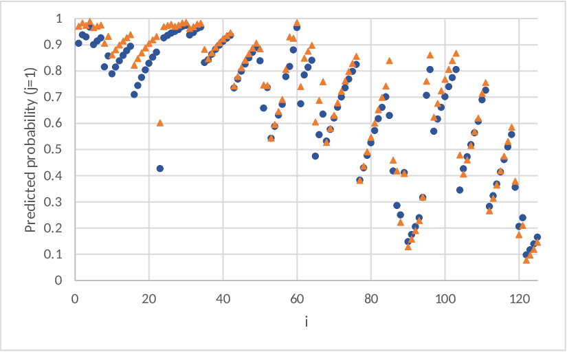
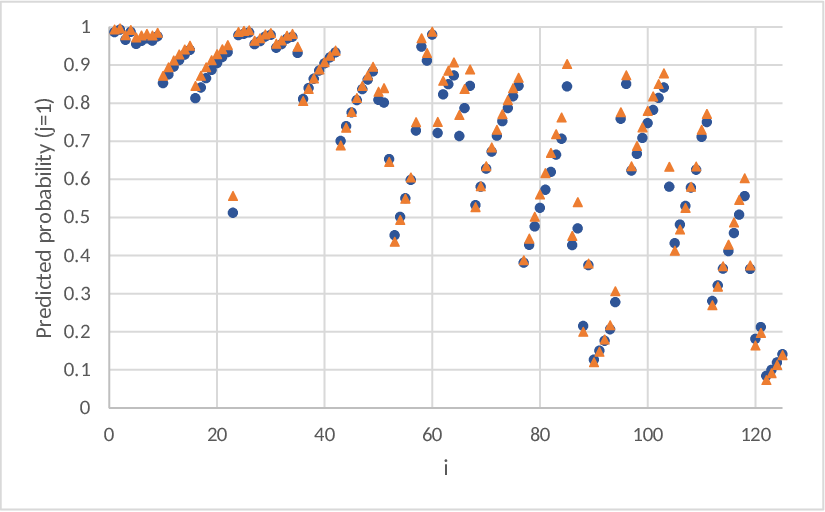
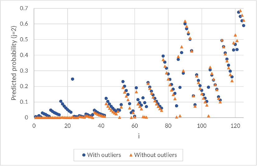
Study of Robustness: From Table 3 in Appendix A.4, the average EMDs in the presence of outliers decrease significantly as λ\lambda increases from 00. This illustrates the increasing robustness of our proposed MDPDEs with increasing λ>0\lambda>0. In order to further examine the robustness of the MDPDEs, we compute the average mean deviations between the predicted probabilities obtained in presence and absence of the outliers, as given by m​d^¯​(𝜷^λp​r​e​s,𝜷^λa​b​s)=1d+1​∑j=1d+1m​d^j​(𝜷^λp​r​e​s,𝜷^λa​b​s)\overline{\widehat{md}}(\widehat{\boldsymbol{\beta}}_{\lambda}^{pres},\widehat{\boldsymbol{\beta}}_{\lambda}^{abs})=\frac{1}{d+1}\sum_{j=1}^{d+1}\widehat{md}_{j}(\widehat{\boldsymbol{\beta}}_{\lambda}^{pres},\widehat{\boldsymbol{\beta}}_{\lambda}^{abs}) with m​d^j​(𝜷^λp​r​e​s,𝜷^λa​b​s)=1N​∑i=1N|πi​j​(𝜷^λp​r​e​s)−πi​j​(𝜷^λa​b​s)|\widehat{md}_{j}(\widehat{\boldsymbol{\beta}}_{\lambda}^{pres},\widehat{\boldsymbol{\beta}}_{\lambda}^{abs})=\dfrac{1}{N}\sum_{i=1}^{N}\left|\pi_{ij}(\widehat{\boldsymbol{\beta}}_{\lambda}^{pres})-\pi_{ij}(\widehat{\boldsymbol{\beta}}_{\lambda}^{abs})\right|, j=1,2,3j=1,2,3. Their values, as presented in Table 4 of Appendix A.4, clearly show that the MDPDE becomes more robust as λ\lambda increases. This behavior is also illustrated in Figure 2, where predicted category probabilities at each observed covariate values are shown for λ=0\lambda=0 (MLE, left) and λ=0.7\lambda=0.7 (right). The differences between blue and orange points, corresponding to the outlier deleted data and the full data, respectively, are quite significant for the classical MLE but much more stable for the MDPDE at λ=0.7\lambda=0.7.

Refer to caption Refer to caption
Figure 2: Predicted category probabilities of the response variable, based on the MLE (left) and the MDPDE with λ=0.7\lambda=0.7 (right), for the three categories (jj) of the Mammography experience data [Blue circles: Full data; Orange triangles: Outlier deleted data].

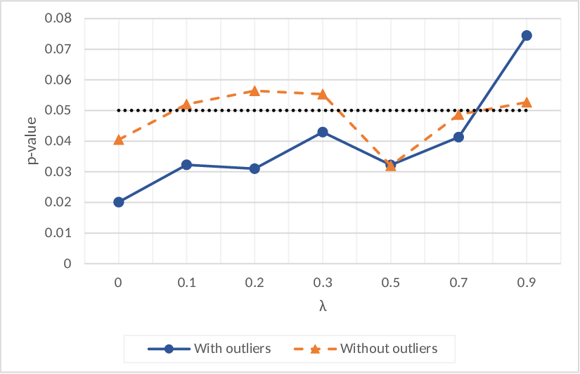
As an illustration of the proposed Wald-type test for this dataset, we consider the problem of testing H0:βS​Y​M​P​T​1,1=0H_{0}:\beta_{SYMPT1,1}=0. The p-values obtained based on the proposed test are plotted over λ\lambda in Figure 3 (left) for both the full and the outlier deleted data. Clearly the test decision at the significance level α=0.05\alpha=0.05 changes completely in the presence of outliers for smaller λ\lambda including the classical Wald test at λ=0\lambda=0. But the inference becomes much stable for larger λ≥0.3\lambda\geq 0.3 implying strong robustness of our proposal.

Refer to caption
Refer to caption
Figure 3: P-values of the proposed MDPDE based Wald-type tests for testing (a) H0:βS​Y​M​P​T​11=0H_{0}:\beta_{SYMPT11}=0 in the Mammography data (left) and (b) H0:β02=0H_{0}:\beta_{02}=0 in the Liver enzyme data (right).

5.2 Liver enzyme data (Plomteux)

Plomteux (1980) showed that the four levels of hepatitis can be explained based on three liver function tests: aspartate aminotransferase (AST), alanine aminotransferase (ALT) and glutamate dehygrogenase (GIDH). The associated dataset (Albert and Harris, 1987) consists of 218 patients with their hepatitis level being categorized as 1 = acute viral hepatitis, 2 = persistent chronic hepatitis, 3 = aggressive chronic hepatitis and 4 = post-necrotic cirrhosis (d=3d=3). Their respective category frequencies are 57, 44, 40 and 77. This dataset has been studied in the literature by Muñoz-Pichardo et al (2011) and Martín (2015), among others.

Here, we model these data with a PLRM where explanatory variables are taken to be the logarithms of the three liver function tests, namely 𝒙=(1,logCLOSE\boldsymbol{x}=(1,\mathrm{log} A​S​T,logAST,\mathrm{log} A​L​T,logALT,\mathrm{log} OPENG​L​D​H)TGLDH)^{T}. As suggested in Martín (2015), the observations associated with indices 93, 101, 108, 116, 131 and 136 of the explanatory variables can be considered as outliers. Table 5 in Appendix A.4 shows the MDPDEs of the model parameters in presence or absence of the outliers, while Table 6 in Appendix A.4 shows the EMDs of the predicted probabilities with respect to the relative frequencies. In this case, all the MDPDEs present a more efficient behavior than MLE even after removing the aforementioned outliers; this indicates that perhaps there are still some masked outliers left in the data which were unidentified by the previous studies. The advantage of the proposed MDPDEs under such cases is clearly evident from this analysis.

Table 7 in Appendix A.4 shows the EMDs between the predicted probabilities obtained from the full data and the outlier deleted data. Again, moderate and large values of λ>0\lambda>0 yield lesser deviation than that for the MLE, indicating their strong robustness against outliers. For testing H0:β02=0H_{0}:\beta_{02}=0, the p-values of the proposed Wald-type tests are plotted in Figure 3. Note that, for λ=0.5\lambda=0.5 the p-values coincide for both the cases with or without outliers.

6 Simulation Study

6.1 Performance of the MDPDE

We consider a nominal outcome variable 𝒀\boldsymbol{Y} with d+1=3d+1=3 categories, depending on k=2k=2 explanatory variables x1x_{1} and x2x_{2}. The true value of the parameter 𝜷=(β01,β11,β21,β02,β12,β22)T\boldsymbol{\beta}=(\beta_{01},\beta_{11},\beta_{21},\beta_{02},\beta_{12},\beta_{22})^{T} is taken as 𝜷0=(0,−0.9,0.1,0.6,−1.2,0.8)T\boldsymbol{\beta}_{0}=(0,-0.9,0.1,0.6,-1.2,0.8)^{T}. We first simulate pure samples of size NN based on covariates xi​1∼𝒩⁡(0,1)x_{i1}\sim\mathcal{N}(0,1), xi​2∼𝒩⁡(0,1)x_{i2}\sim\mathcal{N}(0,1) and the multinomial responses

𝒚i∼ℳ(1;πi​1(𝜷0),πi​2(𝜷0),1−πi​1(𝜷0)−πi​2(𝜷0)),i=1,…,N.\boldsymbol{y}_{i}\sim\mathcal{M}\left(1;\pi_{i1}(\boldsymbol{\beta}_{0}),\pi_{i2}(\boldsymbol{\beta}_{0}),1-\pi_{i1}(\boldsymbol{\beta}_{0})-\pi_{i2}(\boldsymbol{\beta}_{0})\right),~~i=1,\dots,N.

Then, to study the robustness, we additionally change the last p%p\% of responses according to

𝒚i\displaystyle\boldsymbol{y}_{i} ∼\displaystyle\sim ℳ⁡(1,1−πi​1​(𝜷0)−πi​2​(𝜷0),πi​1​(𝜷0),πi​2​(𝜷0)),i=[p100​N]+1,…,N.\displaystyle\mathcal{M}\left(1;1-\pi_{i1}(\boldsymbol{\beta}_{0})-\pi_{i2}(\boldsymbol{\beta}_{0}),\pi_{i1}(\boldsymbol{\beta}_{0}),\pi_{i2}(\boldsymbol{\beta}_{0})\right),\quad i=\left[\frac{p}{100}N\right]+1,\dots,N.

Note that, although we have simulated the contaminated observations with a model-misspecification point-of-view, it indeed also covers the cases of category misspecification. This is because, the contaminated responses are generated with permuted class probabilities, so that categories 1, 2, 3 in the original data are now classified as category 2, 3, 1.

The mean square error (MSE) of the MDPDEs are computed based on 10001000 such simulated samples which are plotted in Figure 4 for different NN, λ\lambda and p=5%p=5\% contaminations. In pure data, the MLE (at λ=0\lambda=0) presents the most efficient behavior having the least MSE for each sample sizes, while MDPDEs with larger λ\lambda have slightly larger MSEs. For contaminated data the behavior of the MDPDEs is almost the opposite; the best behavior (least MSE) is obtained for moderate values of λ\lambda. This becomes more clear with larger sample sizes.

6.2 Performance of the MDPDE based Wald-type tests

Let us now empirically study the robustness of the MDPDE based Wald-type tests for the PLRM. The simulation is performed with the same model as in Section 6.1. We first study the observed level (measured as the proportion of test statistics exceeding the corresponding chi-square critical value) of the test under the true null hypothesis H0:β02=0.6H_{0}:\beta_{02}=0.6. The resulting p-values are plotted in Figure 4 for both the pure and the 5%5\% contaminated samples. In contaminated data, the level of the classical Wald test (at λ=0\lambda=0) as well as the proposed Wald-type tests with small λ\lambda break down, while the MDPDE based Wald-type tests for moderate and large positive λ\lambda yield greater stability in their levels.

To investigate the power robustness of these tests, we change the true data generating parameter value to be β02=1.35\beta_{02}=1.35 and the resulting empirical powers are plotted in Figure 4. Again, the classical Wald test (at λ=0\lambda=0) presents the best behavior under pure data, while the Wald-type tests with larger λ>0\lambda>0 lead to better stability in the contaminated samples.

Refer to caption Refer to caption
Figure 4: MSEs (top panel) of the MDPDEs of 𝜷\boldsymbol{\beta} and the simulated levels (middle panel) and powers (bottom panel) of the Wald-type tests under the pure data (left) and the contaminated data (right).

7 On the choice of tuning parameter λ\lambda

Throughout the previous sections, we have noted that the robustness of both the proposed MDPDE and the associated Wald-type tests increase with increasing λ\lambda; but their pure data (asymptotic) efficiency and power decrease slightly. From our empirical analyses, it seems that a moderately large value of λ\lambda is expected to provide the best trade-off for possibly contaminated data. However, a data-driven choice of λ\lambda would be more helpful in practice.

As noted in Section 4, the robustness of the Wald-type test directly depends on that of the MDPDE used. A useful procedure of the data-based selection of λ\lambda for the MDPDE was proposed by Warwick and Jones (2005) under IID data, which is recently extended for the non-homogeneous data by Ghosh and Basu (2013, 2015, 2016) and Basu et al. (2017a). We can adopt a similar approach to obtain a suitable data-driven λ\lambda in our PLRM. In this approach, we minimize an estimate of the asymptotic MSE of the MDPDE 𝜷^λ\widehat{\boldsymbol{\beta}}_{\lambda}, given by MSE⁡(λ)=(𝜷λ−𝜷∗)T​(𝜷λ−𝜷∗)+1N​trace​{𝑱λ−1​(𝜷λ)​𝑽λ​(𝜷λ)​𝑱λ−1​(𝜷λ)}\mathrm{MSE}(\lambda)=\left(\boldsymbol{\beta}_{\lambda}-\boldsymbol{\beta}^{\ast}\right)^{T}\left(\boldsymbol{\beta}_{\lambda}-\boldsymbol{\beta}^{\ast}\right)+\frac{1}{N}\mathrm{trace}\left\{\boldsymbol{J}_{\lambda}^{-1}\left(\boldsymbol{\beta}_{\lambda}\right)\boldsymbol{V}_{\lambda}\left(\boldsymbol{\beta}_{\lambda}\right)\boldsymbol{J}_{\lambda}^{-1}\left(\boldsymbol{\beta}_{\lambda}\right)\right\}, over λ∈[0,1]\lambda\in[0,1], where 𝜷λ\boldsymbol{\beta}_{\lambda} is the asymptotic mean of 𝜷^λ\widehat{\boldsymbol{\beta}}_{\lambda} and 𝜷∗\boldsymbol{\beta}^{\ast} is the true target parameter value. As pointed out by Basu et. al (2017a), the estimation of the variance component should not assume the model to be true for a better robustness trade-off. So, following the general formulation of Ghosh and Basu (2015), model robust estimates of 𝑽λ\boldsymbol{V}_{\lambda} and 𝑱λ\boldsymbol{J}_{\lambda} can be obtained as 𝑽^N,λ=𝛀N,λ​(𝜷^λ)\widehat{\boldsymbol{V}}_{N,\lambda}=\boldsymbol{\Omega}_{N,\lambda}(\widehat{\boldsymbol{\beta}}_{\lambda}) and

𝑱^N,λ\displaystyle\widehat{\boldsymbol{J}}_{N,\lambda} =(λ+1)​𝚿N,λ​(𝜷^λ)+1N​∑i=1NΔ⁡(𝝅i∗​(𝜷^λ))​{∑j=1d+1πi​j​(𝜷^λ)λ+1}⊗𝒙i​𝒙iT\displaystyle=(\lambda+1)\boldsymbol{\Psi}_{N,\lambda}(\widehat{\boldsymbol{\beta}}_{\lambda})+\frac{1}{N}\sum_{i=1}^{N}\Delta\left(\boldsymbol{\pi}_{i}^{\ast}(\widehat{\boldsymbol{\beta}}_{\lambda})\right)\left\{\sum_{j=1}^{d+1}\pi_{ij}(\widehat{\boldsymbol{\beta}}_{\lambda})^{\lambda+1}\right\}\otimes\boldsymbol{x}_{i}\boldsymbol{x}_{i}^{T}
−1N∑i=1N{λ𝒖i(𝒚i∗,𝜷^λ)𝒖i(𝒚i∗,𝜷^λ)T+Δ(𝝅i∗(𝜷^λ))⊗𝒙i𝒙iT}fi(𝒚i∗,𝜷^λ)λ,\displaystyle-\frac{1}{N}\sum_{i=1}^{N}\left\{\lambda\boldsymbol{u}_{i}(\boldsymbol{y}_{i}^{\ast},\widehat{\boldsymbol{\beta}}_{\lambda})\boldsymbol{u}_{i}(\boldsymbol{y}_{i}^{\ast},\widehat{\boldsymbol{\beta}}_{\lambda})^{T}+\Delta\left(\boldsymbol{\pi}_{i}^{\ast}(\widehat{\boldsymbol{\beta}}_{\lambda})\right)\otimes\boldsymbol{x}_{i}\boldsymbol{x}_{i}^{T}\right\}f_{i}(\boldsymbol{y}_{i}^{\ast},\widehat{\boldsymbol{\beta}}_{\lambda})^{\lambda},

where 𝒖i\boldsymbol{u}_{i} and fif_{i} are given in Appendix. Next, for the bias part, we can use the MDPDE 𝜷^λ\widehat{\boldsymbol{\beta}}_{\lambda} to estimate 𝜷λ{\boldsymbol{\beta}}_{\lambda} but there is no clear choice for estimation of 𝜷∗\boldsymbol{\beta}^{\ast}; Warwick and Jones (2005) suggested to estimate 𝜷∗\boldsymbol{\beta}^{\ast} by some appropriate pilot estimator 𝜷P\boldsymbol{\beta}^{P}. Note that, the overall performance of this procedure of selecting optimum λ\lambda depends on the choice of 𝜷P\boldsymbol{\beta}^{P}, which we will explore through an empirical study.

Consider the same simulation study as in Section 6.1. We now compute the optimal λ\lambda value in each iteration following the proposed method with a given 𝜷P\boldsymbol{\beta}^{P}. As potential choices of 𝜷P\boldsymbol{\beta}^{P}, we consider the MDPDEs with “pilot” parameters λp∈{0,0.3,0.5,1}\lambda_{p}\in\{0,0.3,0.5,1\}. For example, when λp=0.5\lambda_{p}=0.5, we fix 𝜷P=𝜷^0.5\boldsymbol{\beta}^{P}=\widehat{\boldsymbol{\beta}}_{0.5} and minimize the estimated quantity MSE^​(λ)=(𝜷^λ−𝜷^0.5)T​(𝜷^λ−𝜷^0.5)+1N​trace​(𝑱^N,λ−1​𝑽^N,λ​𝑱^N​λ−1)\widehat{\mathrm{MSE}}(\lambda)=\left(\widehat{\boldsymbol{\beta}}_{\lambda}-\widehat{\boldsymbol{\beta}}_{0.5}\right)^{T}\left(\widehat{\boldsymbol{\beta}}_{\lambda}-\widehat{\boldsymbol{\beta}}_{0.5}\right)+\frac{1}{N}\mathrm{trace}\left(\widehat{\boldsymbol{J}}_{N,\lambda}^{-1}\widehat{\boldsymbol{V}}_{N,\lambda}\widehat{\boldsymbol{J}}_{N\lambda}^{-1}\right), through a grid search over λ∈[0,1]\lambda\in[0,1], to obtain the optimum λ\lambda value. Note that, the bias term is not generally zero even though we are using MDPDEs as the pilot estimator. Figure 5 shows the empirical MSEs for the final MDPDEs with the resulting optimum λ\lambda (in each iteration) for the pure and the contaminated data. Clearly, the best trade-off between the efficiency in pure data and the robustness under contaminated data is provided by the pilot choice λp=0.3\lambda_{p}=0.3 and the corresponding MSEs are also satisfactorily small in both the cases. So, we suggest to use the pilot choice 𝜷P=𝜷^0.3\boldsymbol{\beta}^{P}=\widehat{\boldsymbol{\beta}}_{0.3} for the PLRM and the steps for the final algorithm are clearly mentioned below.

Algorithm for the data-driven selection of optimum tuning parameter λ\lambda    • Aim: Optimal fitting of the PLRM given a dataset • Fix: Pilot estimate 𝜷P=𝜷^0.3\boldsymbol{\beta}^{P}=\widehat{\boldsymbol{\beta}}_{0.3}.                               (Empirical suggestion) • For each λ\lambda in a grid of [0,1][0,1], do the following.          (E.g., λ\lambda in 0:0.01:10:0.01:1) – Compute the total estimated squared bias B⁡(λ)=(𝜷^λ−𝜷^0.3)T​(𝜷^λ−𝜷^0.3)B(\lambda)=\left(\widehat{\boldsymbol{\beta}}_{\lambda}-\widehat{\boldsymbol{\beta}}_{0.3}\right)^{T}\left(\widehat{\boldsymbol{\beta}}_{\lambda}-\widehat{\boldsymbol{\beta}}_{0.3}\right). – Compute the total estimated variance V⁡(λ)=1N​trace​(𝑱^N,λ−1​𝑽^N,λ​𝑱^N​λ−1)V(\lambda)=\frac{1}{N}\mathrm{trace}\left(\widehat{\boldsymbol{J}}_{N,\lambda}^{-1}\widehat{\boldsymbol{V}}_{N,\lambda}\widehat{\boldsymbol{J}}_{N\lambda}^{-1}\right). – Compute the total estimated MSE as MSE^​(λ)=B⁡(λ)+V⁡(λ)\widehat{\mathrm{MSE}}(\lambda)=B(\lambda)+V(\lambda). • Find: Minimum of MSE^​(λ)\widehat{\mathrm{MSE}}(\lambda) and the corresponding λ\lambda. Let λo​p​t=arg⁡min​MSE^​(λ)\lambda_{opt}=\arg\min\widehat{\mathrm{MSE}}(\lambda). • Return: λo​p​t\lambda_{opt} as the final optimum value of the tuning parameter. • Compute 𝜷^λo​p​t\widehat{\boldsymbol{\beta}}_{\lambda_{opt}} as your final estimate with optimally chosen tuning parameter.

Refer to caption Refer to caption
Figure 5: Simulated MSEs of the MDPDEs at the optimally chosen λ\lambda, starting from different pilot estimators under the pure data (left) and the contaminated data (right).

We now apply this proposed algorithm (with a grid of spacing 0.05) to our real datasets. The optimum λ\lambda turns out to be 11 and 0.750.75, respectively, for the Mammography experience data and the Liver enzyme data in presence of the outliers. After deleting the aforementioned outliers from the data, these optimum λ\lambda values become 0.050.05 and 0.350.35, respectively. These optimum λ\lambda values generate quite stable MDPDEs for both datasets, as we have seen in Section 5. They indeed yield the automatic data-driven choices of λ\lambda which are also consistent with the fact that we should use larger λ>0\lambda>0 for contaminated data and smaller λ\lambda close to zero for clean data. Note that, as discussed in Section 5, the liver enzyme data might contain some masked outlying observations even after removing the aforementioned outliers from previous studies which leads to the slightly larger optimum λ\lambda value of 0.35. These evidences clearly justify the appropriateness and usefulness of our proposed algorithm of selecting optimum data-driven λ\lambda for the MDPDEs in case of the PLRM.

8 Concluding Remarks

The PLRM is an extensively applied statistical tool which is widely used in many different areas, including health and life sciences. Although the classical inference procedures based on the MLE have asymptotic optimal properties, they are highly non-robust against outliers in data. So, there is a strong need for robust procedures in practical applications of the PLRM due to the presence of potential outlying observations in many real datasets. Here we derive a new family of estimators, MDPDEs, as a robust generalization of the MLE for the PLRM, exploring the “nice” robustness properties of the DPD measure. A family of Wald-type test statistics based on the MDPDEs is also introduced for testing linear hypotheses under the PLRM. The study of two real data examples from medical sciences as well as the simulation results illustrate the advantages of our proposed inference procedures.

Acknowledgements

We would like to thank the Editor, the Associate Editor and the Referees for their helpful comments and suggestions. This research is supported by Grant MTM2015-67057-P, from Ministerio de Economia y Competitividad (Spain) and by the INSPIRE Faculty Research Grant from Department of Science & Technology, Govt. of India.

References

  • [1] Aerts, S. and Haesbroeck, G. (2017). Robust asymptotic tests for the equality of multivariate coefficients of variation. TEST 26(1), 163–187.
  • [2] Albert, A. and Harris, E.K. (1987). Multivariate interpretation of clinical laboratory data, New York: Marcel Dekker.
  • [3] Basu, A., Shioya, H. and Park, C. (2011). The minimum distance approach. Monographs on Statistics and Applied Probability. CRC Press, Boca Raton.
  • [4] Basu, A., Mandal, A., Martín, N. and Pardo, L. (2016). Generalized Wald-type tests based on minimum density power divergence estimators. Statistics 50, 1–26.
  • [5] Basu, A. Ghosh, A. Mandal, Martin, N. and Pardo, L. (2017a). A Wald-type test statistic for testing linear hypothesis in logistic regression models based on minimum density power divergence estimator. Electonic Journal of Statistics 11, 2741-2772.
  • [6] Basu, A., Ghosh, A., Martin, N. and Pardo, L. (2017b). Robust Wald-type tests for non-homogeneous observations based on minimum density power divergence estimator. ArXiv pre-print, arXiv:1707.02333 [stat.ME].
  • [7] Begg, C.B. and Gray, R. (1984). Calculations of polychotomous logistic regression estimates using individualized regressions. Biometrika 71, 1-18.
  • [8] Bertens, L. C. M., Moons, K. G. M., Rutten, F. H. van Mourik, I., Hoes, A. W. and Reitsma, J. B. (2015). A nomogram was developed to enhance the use of multinomial logistic regression modeling in diagnostic research. Journal of Clinical Epidemiology 71, 51–57.
  • [9] Biesheuvel, C.J., Vergouwe, Y., Steyerberg, E.W., Grobbee, D.E. and Moons, K.G. (2008). Polytomous logistic regression analysis could be applied more often in diagnostic research. Journal of Clinical Epidemiology 61, 125-134.
  • [10] Blizzard, L. and Hosmer, D. W. (2007). The Log Multinomial Regression Model for Nominal Outcomes with More than Two Attributes. Biometrical Journal 49, 889–902.
  • [11] Bull, S. B., Lewinger, J. P. and Lee, S. S. F. (2007). Confidence intervals for multinomial logistic regression in sparse data. Statistics in Medicine 26, 903–918.
  • [12] Daniels, M. J. and Gatsonis, C. (1997). Hierarchical polytomous regression models with applications to health services research. Statistics in Medicine 16, 2311–2325.
  • [13] Dey, S., Raheem, E. and Lu, Z. (2016). Multilevel multinomial logistic regression model for identifying factors associated with anemia in children 6–59 months in northeastern states of India. Cogent Mathematics 3, 1-12.
  • [14] Dreassi, D. (2007). Polytomous Disease Mapping to Detect Uncommon Risk Factors for Related Diseases. Biometrical Journal 49, 520–529.
  • [15] Ghosh, A. and Basu, A. (2013). Robust Estimation for Independent but Non-Homogeneous Observations using Density Power Divergence with application to Linear Regression. Electonic Journal of Statistics 7, 2420–2456.
  • [16] Ghosh, A. and Basu, A. (2015). Robust estimation for non-homogeneous data and the selection of the optimal tuning parameter: the density power divergence approach. Journal of Applied Statitsics 42(9), 2056–2072.
  • [17] Ghosh, A. and Basu, A. (2016). Robust Estimation in Generalized Linear Models: The density power divergence. TEST 25, 269-290.
  • [18] Ghosh, A., and Basu, A. (2017). Robust Bounded Influence Tests for Independent but Non-Homogeneous Observations. Statistica Sinica doi:10.5705/ss.202015.0320.
  • [19] Ghosh, A., Mandal, A., Martín, N. and Pardo, L. (2016). Influence Analysis of Robust Wald-type Tests. Journal Multivariate Analysis 147, 102–126.
  • [20] Gupta, A. K., Kasturiratna, D., Nguyen, T. and Pardo, L. (2006). A new family of BAN estimators for polytomous logistic regression models based on ϕ\phi-divergence measures. Statistical Methods & Applications 15, 159–176.
  • [21] Hayashi, F. (2000). Econometrics. New Jersey: Princeton University Press.
  • [22] Hosmer, D.W. and Lemeshow, S. (2000). Applied logistic regression. Wiley, New York.
  • [23] Huber, P. J. (1983). Minimax aspects of bounded-influence regression (with discussion). Journal of the American Statistical Association 78, 66-80.
  • [24] Ke, Y., Fu, B. and Zhang, W. (2016). Semi-varying coefficient multinomial logistic regression for disease progression risk prediction. Statistics in Medicine 35, 4764–4778.
  • [25] Martín, N. (2015). Using Cook’s distance in polytomous logistic regression. British Journal of Mathematical and Statistical Psychology 68, 84–115.
  • [26] Muñoz-Pichardo, J. M. ; Enguix-Gonzalez, A.; Muñoz-García, J. and Moreno-Rebollo, J. L. (2011). Infuence analysis on discriminant coordinates. Communications in Statistics - Simulation and Computation 40, 793-807.
  • [27] Nelder, J. A. and Wedderburn, R. W. M. (1972). Generalized Linear Models. London, Chapman & Hall.
  • [28] Pardo, L. (2005). Statistical Inference Based on Divergence Measures. Statistics: Texbooks and Monographs. Chapman & Hall/CRC, New York.
  • [29] Plomteux, G. (1980). Multivariate analysis of an enzyme profile for the differential diagnosis of viral hepatitis. Clinical Chemistry 26, 1897–1899.
  • [30] Rom, M. and Cohen, A. (1995). Estimation in the polytomous logistic regression models, Journal of Statistical Planning and Inference 43, 341-353.
  • [31] Ronchetti, E. and Trojani, F. (2001). Robust inference with gmm estimators. Journal of Econometrics 101, 37–69.
  • [32] Rousseeuw, P. J. and Ronchetti, E. (1979). The influence curve for tests. Research Report 21, Fachgruppe fur Statistik, ETH Zurich.
  • [33] Victoria-Feser, M. and Ronchetti, E. (1997). Robust estimation for grouped data. Journal of the American Statistical Association 92, 333–340.
  • [34] Wang, X. (2014). Modified generalized method of moments for a robust estimation of polytomous logistic model. PeerJ 2:e467 https://doi.org/10.7717/peerj.467
  • [35] Warwick, J., and Jones, M. C. (2005). Choosing a robustness tuning parameter. Journal of Statistical Computation and Simulation, 75, 581–588.

Appendix A Supplementary Materials: Appendices and Tables referenced in Sections 3, 5 6 and 7

A.1 How to obtain the MDPDEs?

Consider the set-up and notations of Section 2 of the main paper. The following theorem presents the estimating equation for the MDPDEs in the PLRM, which can be solved numerically to obtain the estimates.

Theorem 6

The MDPDE, 𝛃^λ\widehat{\boldsymbol{\beta}}_{\lambda}, of 𝛃\boldsymbol{\beta} can be obtained by solving the system of equations

𝒖λ​(𝜷)=𝟎d⁡(k+1),\boldsymbol{u}_{\lambda}\left(\boldsymbol{\beta}\right)=\boldsymbol{0}_{d(k+1)},

where

𝒖λ​(𝜷)=∑i=1N[(𝑰d,𝟎d)​𝚫​(𝝅i​(𝜷))​diagλ−1​{𝝅i​(𝜷)}​{𝒚i−𝝅i​(𝜷)}]⊗𝒙i\boldsymbol{u}_{\lambda}\left(\boldsymbol{\beta}\right)=\sum_{i=1}^{N}\left[\left(\boldsymbol{I}_{d},\boldsymbol{0}_{d}\right)\boldsymbol{\Delta}(\boldsymbol{\pi}_{i}\left(\boldsymbol{\beta}\right))\mathrm{diag}^{\lambda-1}\{\boldsymbol{\pi}_{i}\left(\boldsymbol{\beta}\right)\}\{\boldsymbol{y}_{i}-\boldsymbol{\pi}_{i}\left(\boldsymbol{\beta}\right)\}\right]\otimes\boldsymbol{x}_{i}

Proof. The MDPDE of 𝜷\boldsymbol{\beta}, is defined as

𝜷^λ\displaystyle\widehat{\boldsymbol{\beta}}_{\lambda} =arg⁡min𝜷∈ℝd⁡(k+1)​∑i=1N{𝝅i​(𝜷)−λ+1λ​𝒚i}T​𝝅i(λ)​(𝜷)\displaystyle=\underset{\boldsymbol{\beta}\in\mathbb{R}^{d(k+1)}}{\arg\min}\sum_{i=1}^{N}\left\{\boldsymbol{\pi}_{i}\left(\boldsymbol{\beta}\right)-\frac{\lambda+1}{\lambda}\boldsymbol{y}_{i}\right\}^{T}\boldsymbol{\pi}_{i}^{(\lambda)}\left(\boldsymbol{\beta}\right)
=arg⁡min𝜷∈ℝd⁡(k+1)​∑i=1N∑j=1d+1{πi​jλ+1​(𝜷)−λ+1λ​yi​j​πi​jλ​(𝜷)},\displaystyle=\underset{\boldsymbol{\beta}\in\mathbb{R}^{d(k+1)}}{\arg\min}\sum_{i=1}^{N}\sum_{j=1}^{d+1}\left\{\pi_{ij}^{\lambda+1}(\boldsymbol{\beta})-\frac{\lambda+1}{\lambda}y_{ij}\pi_{ij}^{\lambda}(\boldsymbol{\beta})\right\},

which can also be obtained by solving the system of equations 𝒖λ​(𝜷)=𝟎d⁡(k+1)\boldsymbol{u}_{\lambda}\left(\boldsymbol{\beta}\right)=\boldsymbol{0}_{d(k+1)} where

−1λ+1∂∂𝜷∑i=1N{𝝅i(𝜷)−λ+1λ𝒚i}T𝝅i(λ)(𝜷)\displaystyle-\frac{1}{\lambda+1}\frac{\partial}{\partial\boldsymbol{\beta}}\sum_{i=1}^{N}\left\{\boldsymbol{\pi}_{i}\left(\boldsymbol{\beta}\right)-\frac{\lambda+1}{\lambda}\boldsymbol{y}_{i}\right\}^{T}\boldsymbol{\pi}_{i}^{(\lambda)}\left(\boldsymbol{\beta}\right) =𝟎d⁡(k+1),\displaystyle=\boldsymbol{0}_{d(k+1)},
∑i=1N∑j=1d+1{yi​j−πi​j​(𝜷)}​πi​jλ+1​(𝜷)​∂∂𝜷​πi​j​(𝜷)\displaystyle\sum_{i=1}^{N}\sum_{j=1}^{d+1}\{y_{ij}-\pi_{ij}(\boldsymbol{\beta})\}\pi_{ij}^{\lambda+1}(\boldsymbol{\beta})\frac{\partial}{\partial\boldsymbol{\beta}}\pi_{ij}(\boldsymbol{\beta}) =𝟎d⁡(k+1),\displaystyle=\boldsymbol{0}_{d(k+1)},
∑i=1N∂∂𝜷​𝝅i​(𝜷)T​diagλ−1​{𝝅i​(𝜷)}​{𝒚i−𝝅i​(𝜷)}\displaystyle\sum_{i=1}^{N}\frac{\partial}{\partial\boldsymbol{\beta}}\boldsymbol{\pi}_{i}\left(\boldsymbol{\beta}\right)^{T}\mathrm{diag}^{\lambda-1}\{\boldsymbol{\pi}_{i}\left(\boldsymbol{\beta}\right)\}\{\boldsymbol{y}_{i}-\boldsymbol{\pi}_{i}\left(\boldsymbol{\beta}\right)\} =𝟎d⁡(k+1).\displaystyle=\boldsymbol{0}_{d(k+1)}.

Now, taking into account that

∂πi​j​(𝜷)∂βu​v=xi​uπi​j(𝜷){δj​v−πi​v(𝜷)},u=1,…,k,v=1,…,d,\frac{\partial\pi_{ij}(\boldsymbol{\beta})}{\partial\beta_{uv}}=x_{iu}\pi_{ij}(\boldsymbol{\beta})\left\{\delta_{jv}-\pi_{iv}(\boldsymbol{\beta})\right\},\qquad u=1,...,k,v=1,...,d,

we get

∂𝝅i​(𝜷)T∂𝜷=(𝑰d,𝟎d)​𝚫​(𝝅i​(𝜷))⊗𝒙i,\frac{\partial\boldsymbol{\pi}_{i}(\boldsymbol{\beta})^{T}}{\partial\boldsymbol{\beta}}=\left(\boldsymbol{I}_{d},\boldsymbol{0}_{d}\right)\boldsymbol{\Delta}(\boldsymbol{\pi}_{i}\left(\boldsymbol{\beta}\right))\otimes\boldsymbol{x}_{i}, (9)

and hence the system of equations becomes

∑i=1N[(𝑰d,𝟎d)​𝚫​(𝝅i​(𝜷))​diagλ−1​{𝝅i​(𝜷)}​{𝒚i−𝝅i​(𝜷)}]⊗𝒙i=𝟎d⁡(k+1).\sum_{i=1}^{N}\left[\left(\boldsymbol{I}_{d},\boldsymbol{0}_{d}\right)\boldsymbol{\Delta}(\boldsymbol{\pi}_{i}\left(\boldsymbol{\beta}\right))\mathrm{diag}^{\lambda-1}\{\boldsymbol{\pi}_{i}\left(\boldsymbol{\beta}\right)\}\{\boldsymbol{y}_{i}-\boldsymbol{\pi}_{i}\left(\boldsymbol{\beta}\right)\}\right]\otimes\boldsymbol{x}_{i}=\boldsymbol{0}_{d(k+1)}.


Note that, under the PLRM, the tabulated response variables 𝒀i\boldsymbol{Y}_{i}, i=1,…,Ni=1,...,N, are independent but not identically distributed since the covariates 𝒙i\boldsymbol{x}_{i} are generally assumed to be pre-fixed (and hence different over ii). In particular, for each i=1,…,Ni=1,\ldots,N, given 𝒙i\boldsymbol{x}_{i}, 𝒀i\boldsymbol{Y}_{i} has a multinomial distribution having joint probability mass function

fi(𝒚i,𝜷)=∏j=1d+1πi​j(𝜷)yi​j=∑j=1d+1yi​jπi​j(𝜷),yi​j∈{0,1} for j=1,…,d+1, with ∑j=1d+1yi​j=1.f_{i}(\boldsymbol{y}_{i},\boldsymbol{\beta})=\prod_{j=1}^{d+1}\pi_{ij}\left(\boldsymbol{\beta}\right)^{y_{ij}}=\sum_{j=1}^{d+1}{y_{ij}}\pi_{ij}\left(\boldsymbol{\beta}\right),\quad y_{ij}\in\{0,1\}\text{ for }j=1,\ldots,d+1\text{, with }\sum_{j=1}^{d+1}y_{ij}=1. (10)

This distribution indeed belongs to the family of dd-dimensional Generalized Linear Models (GLM), where the distribution of 𝒀i∗=(Yi​1,…,Yi​d)T\boldsymbol{Y}_{i}^{\ast}=(Y_{i1},\dots,Y_{id})^{T} can be written as

fi​(𝒚i∗,𝜷)\displaystyle f_{i}(\boldsymbol{y}_{i}^{\ast},\boldsymbol{\beta}) =exp⁡{𝜼iT​𝒚i∗−b⁡(𝜼i)},\displaystyle=\exp\left\{\boldsymbol{\eta}_{i}^{T}\boldsymbol{y}_{i}^{\ast}-b(\boldsymbol{\eta}_{i})\right\},
𝜼i\displaystyle\boldsymbol{\eta}_{i} =(ηi​1,…,ηi​d)T,ηi​j=𝒙iT𝜷j, j=1,…,d,\displaystyle=(\eta_{i1},...,\eta_{id})^{T},\quad\eta_{ij}=\boldsymbol{x}_{i}^{T}\boldsymbol{\beta}_{j},\text{ }j=1,...,d,
b⁡(𝜼i)\displaystyle b(\boldsymbol{\eta}_{i}) =log⁡{1+∑j=1dexp⁡(ηi​j)}.\displaystyle=\log\left\{1+\sum_{j=1}^{d}\exp(\eta_{ij})\right\}.

The general estimating equation of Ghosh and Basu (2013), based on these forms of the model densities, can be seen to coincide with the one given in Theorem 1.

A.2 Power function of the Wald-type tests

Consider the set-up and notations of Section 3 of the main paper. We consider 𝜷∗\boldsymbol{\beta}_{\ast} ∈Θ\in\Theta such that 𝑳T​𝜷∗≠𝒉,\boldsymbol{L}^{T}\boldsymbol{\beta}_{\ast}\neq\boldsymbol{h,} i.e., 𝜷∗\boldsymbol{\beta}_{\ast} does not satisfy the null hypothesis given in Equation (6) of the main paper. Let us denote

q𝜷1​(𝜷2)=(𝑳T​𝜷1−𝒉)T​{𝑳T​𝚺λ​(𝜷2)​𝑳}−1​(𝑳T​𝜷1−𝒉)q_{\boldsymbol{\beta}_{1}}({\boldsymbol{\beta}_{2}})=\left(\boldsymbol{L}^{T}\boldsymbol{\beta}_{1}-\boldsymbol{h}\right)^{T}\left\{\boldsymbol{L}^{T}\boldsymbol{\Sigma}_{\lambda}\left(\boldsymbol{\beta}_{2}\right)\boldsymbol{L}\right\}^{-1}\left(\boldsymbol{L}^{T}\boldsymbol{\beta}_{1}-\boldsymbol{h}\right) (11)

and derive an approximation to the power function for the MDPDE based Wald-type test with the rejection rule given by

WN​(𝜷^λ)>χr,α2.W_{N}(\widehat{\boldsymbol{\beta}}_{\lambda})>\chi_{r,\alpha}^{2}. (12)
Theorem 7

Let 𝛃∗∈Θ\boldsymbol{\beta}_{\ast}\in\Theta, with 𝐋T​𝛃∗≠𝐡\boldsymbol{L}^{T}\boldsymbol{\beta}_{\ast}\neq\boldsymbol{h}, be the true value of the parameter such that 𝛃^λ​⟶N→∞𝑃​𝛃∗\widehat{\boldsymbol{\beta}}_{\lambda}\underset{N\rightarrow\infty}{\overset{P}{\longrightarrow}}\boldsymbol{\beta}_{\ast}. The power function of the Wald-type test given in (12), is given by

βN,λ​(𝜷∗)=1−ΦN​(1σλ​(𝜷∗)​(χs,α2N−N​q𝜷∗​(𝜷∗)))\beta_{N,\lambda}\left(\boldsymbol{\beta}_{\ast}\right)=1-\Phi_{N}\left(\frac{1}{\sigma_{\lambda}\left(\boldsymbol{\beta}_{\ast}\right)}\left(\frac{\chi_{s,\alpha}^{2}}{\sqrt{N}}-\sqrt{N}q_{\boldsymbol{\beta}_{\ast}}(\boldsymbol{\beta}_{\ast})\right)\right) (13)

where ΦN​(x)\Phi_{N}\left(x\right) uniformly tends to the standard normal distribution function Φ⁡(x)\Phi(x) as N→∞N\rightarrow\infty and

σλ​(𝜷∗)=2​(𝑳T​𝜷∗−𝒉)T​{𝑳T​𝚺λ​(𝜷∗)​𝑳}−1​(𝑳T​𝜷∗−𝒉).\sigma_{\lambda}\left(\boldsymbol{\beta}_{\ast}\right)=2\sqrt{\left(\boldsymbol{L}^{T}\boldsymbol{\beta}_{\ast}-\boldsymbol{h}\right)^{T}\left\{\boldsymbol{L}^{T}\boldsymbol{\Sigma}_{\lambda}\left(\boldsymbol{\beta}_{\ast}\right)\boldsymbol{L}\right\}^{-1}\left(\boldsymbol{L}^{T}\boldsymbol{\beta}_{\ast}-\boldsymbol{h}\right)}.

Proof. We have

βN,λ​(𝜷∗)\displaystyle\beta_{N,\lambda}\left(\boldsymbol{\beta}_{\ast}\right) =Pr⁡(WN​(𝜷^λ)>χr,α2)=Pr⁡(N⁡(q𝜷^λ​(𝜷^λ)−q𝜷∗​(𝜷∗))>χr,α2−N​q𝜷∗​(𝜷∗))\displaystyle=\Pr\left(W_{N}(\widehat{\boldsymbol{\beta}}_{\lambda})>\chi_{r,\alpha}^{2}\right)=\Pr\left(N\left(q_{\widehat{\boldsymbol{\beta}}_{\lambda}}(\widehat{\boldsymbol{\beta}}_{\lambda})-q_{\boldsymbol{\beta}_{\ast}}(\boldsymbol{\beta}_{\ast})\right)>\chi_{r,\alpha}^{2}-Nq_{\boldsymbol{\beta}_{\ast}}(\boldsymbol{\beta}_{\ast})\right)
=Pr⁡(N​(q𝜷^λ​(𝜷^λ)−q𝜷∗​(𝜷∗))>χr,α2N−N​q𝜷∗​(𝜷∗)).\displaystyle=\Pr\left(\sqrt{N}\left(q_{\widehat{\boldsymbol{\beta}}_{\lambda}}(\widehat{\boldsymbol{\beta}}_{\lambda})-q_{\boldsymbol{\beta}_{\ast}}(\boldsymbol{\beta}_{\ast})\right)>\frac{\chi_{r,\alpha}^{2}}{\sqrt{N}}-\sqrt{N}q_{\boldsymbol{\beta}_{\ast}}(\boldsymbol{\beta}_{\ast})\right).

Note that, since 𝜷^λ​⟶N→∞𝑃​𝜷∗\widehat{\boldsymbol{\beta}}_{\lambda}\underset{N\rightarrow\infty}{\overset{P}{\longrightarrow}}\boldsymbol{\beta}_{\ast}, q𝜷^λ​(𝜷^λ)q_{\widehat{\boldsymbol{\beta}}_{\lambda}}(\widehat{\boldsymbol{\beta}}_{\lambda}) and q𝜷^λ​(𝜷∗)q_{\widehat{\boldsymbol{\beta}}_{\lambda}}(\boldsymbol{\beta}_{\ast}) have the same asymptotic distribution. But, a first Taylor expansion of qβ​(𝜷∗)q_{\beta}(\boldsymbol{\beta}_{\ast}) around 𝜷∗\boldsymbol{\beta}^{\ast} at 𝜷^λ\widehat{\boldsymbol{\beta}}_{\lambda} gives

q𝜷^λ​(𝜷∗)−q𝜷∗​(𝜷∗)=∂q𝜷​(𝜷∗)∂𝜷T|𝜷=𝜷∗​(𝜷^λ−𝜷∗)+op​(‖𝜷^λ−𝜷∗‖).q_{\widehat{\boldsymbol{\beta}}_{\lambda}}(\boldsymbol{\beta}_{\ast})-q_{\boldsymbol{\beta}_{\ast}}(\boldsymbol{\beta}_{\ast})=\left.\frac{\partial q_{\boldsymbol{\beta}}(\boldsymbol{\beta}_{\ast})}{\partial\boldsymbol{\beta}^{T}}\right|_{\boldsymbol{\beta}=\boldsymbol{\beta}_{\ast}}(\widehat{\boldsymbol{\beta}}_{\lambda}-\boldsymbol{\beta}_{\ast})+o_{p}\left(\left\|\widehat{\boldsymbol{\beta}}_{\lambda}-\boldsymbol{\beta}_{\ast}\right\|\right).

Therefore,

N​(q𝜷^λ​(𝜷^∗)−q𝜷∗​(𝜷∗))​⟶N→∞ℒ​𝒩​(0,σλ​(𝜷∗)2)\sqrt{N}(q_{\widehat{\boldsymbol{\beta}}_{\lambda}}(\widehat{\boldsymbol{\beta}}_{\ast})-q_{\boldsymbol{\beta}_{\ast}}(\boldsymbol{\beta}_{\ast}))\overset{\mathcal{L}}{\underset{N\rightarrow\infty}{\longrightarrow}}\mathcal{N}\left(0,\sigma_{\lambda}\left(\boldsymbol{\beta}_{\ast}\right)^{2}\right)

where

σλ​(𝜷∗)2=∂q𝜷​(𝜷∗)∂𝜷T|𝜷=𝜷∗​𝚺λ​(𝜷∗)​∂q𝜷​(𝜷∗)∂𝜷|𝜷=𝜷∗.\sigma_{\lambda}\left(\boldsymbol{\beta}_{\ast}\right)^{2}=\left.\frac{\partial q_{\boldsymbol{\beta}}(\boldsymbol{\beta}_{\ast})}{\partial\boldsymbol{\beta}^{T}}\right|_{\boldsymbol{\beta}=\boldsymbol{\beta}_{\ast}}\boldsymbol{\Sigma}_{\lambda}\left(\boldsymbol{\beta}_{\ast}\right)\left.\frac{\partial q_{\boldsymbol{\beta}}(\boldsymbol{\beta}_{\ast})}{\partial\boldsymbol{\beta}}\right|_{\boldsymbol{\beta}=\boldsymbol{\beta}_{\ast}}.

But

∂q𝜷​(𝜷∗)∂𝜷T|𝜷=𝜷∗T=2​(𝑳T​𝜷∗−𝒉)​{𝑳T​𝚺λ​(𝜷∗)​𝑳}−1​𝑳T,\left.\frac{\partial q_{\boldsymbol{\beta}}(\boldsymbol{\beta}_{\ast})}{\partial\boldsymbol{\beta}^{T}}\right|_{\boldsymbol{\beta}=\boldsymbol{\beta}_{\ast}}^{T}=2\left(\boldsymbol{L}^{T}\boldsymbol{\beta}_{\ast}-\boldsymbol{h}\right)\left\{\boldsymbol{L}^{T}\boldsymbol{\Sigma}_{\lambda}\left(\boldsymbol{\beta}_{\ast}\right)\boldsymbol{L}\right\}^{-1}\boldsymbol{L}^{T},

and hence the result follows.  

Remark 8

Based on the previous theorem we can obtain the minimum sample size which is necessary to achieve a fix power, say βN,λ​(𝛃∗)=β¯\beta_{N,\lambda}\left(\boldsymbol{\beta}_{\ast}\right)=\overline{\beta}. Based in equation (13), we must solve the equation

1−β¯=Φ⁡(1σλ​(𝜷∗)​(χr,α2N−N​q𝜷∗​(𝜷∗)))1-\overline{\beta}=\Phi\left(\frac{1}{\sigma_{\lambda}\left(\boldsymbol{\beta}_{\ast}\right)}(\tfrac{\chi_{r,\alpha}^{2}}{\sqrt{N}}-\sqrt{N}q_{\boldsymbol{\beta}_{\ast}}(\boldsymbol{\beta}_{\ast}))\right)

and we get that N=[N∗]+1N=\left[N^{\ast}\right]+1 with

N∗=A+B+A⁡(A+2​B)2​q𝜷∗​(𝜷∗)2N^{\ast}=\frac{A+B+\sqrt{A(A+2B)}}{2q_{\boldsymbol{\beta}_{\ast}}({\boldsymbol{\beta}_{\ast}})^{2}}

being A=σλ​(𝛃∗)2​(Φ−1​(1−β¯))2A=\sigma_{\lambda}\left(\boldsymbol{\beta}_{\ast}\right)^{2}\left(\Phi^{-1}\left(1-\overline{\beta}\right)\right)^{2} and B=12​χr,α2​q𝛃∗​(𝐶𝐿𝑂𝑆𝐸B=\frac{1}{2}\chi_{r,\alpha}^{2}q_{\boldsymbol{\beta}_{\ast}}(𝛃∗\boldsymbol{\beta}_{\ast})) and q𝛃∗​(𝐶𝐿𝑂𝑆𝐸q_{\boldsymbol{\beta}_{\ast}}(𝛃∗\boldsymbol{\beta}_{\ast})) is given in (11).

Remark 9

It also follows from Theorem 7 that βN,λ​(β∗)→1\beta_{N,\lambda}(\beta^{\ast})\rightarrow 1, as N→∞N\rightarrow\infty, for all λ≥0\lambda\geq 0. Therefore the proposed MDPDE based Wald-type tests are consistent at any fixed alternative.

We now derive the asymptotic power function for the Wald-type test with the rejection rule given in (12) at an alternative hypothesis close to the null hypothesis. Consider the parameter value 𝜷N∈Θ\boldsymbol{\beta}_{N}\in\Theta with 𝑳T​𝜷\boldsymbol{L}^{T}\boldsymbol{\beta} 𝑵≠𝒉\boldsymbol{{}_{N}}\neq\boldsymbol{h}, and the alternative hypothesis given by 𝜷=𝜷N\boldsymbol{\beta}=\boldsymbol{\beta}_{N}. Suppose 𝜷0\boldsymbol{\beta}_{0} be the closest parameter value to 𝜷N\boldsymbol{\beta}_{N} in the Euclidean distance such that 𝑳T​𝜷0=𝒉\boldsymbol{L}^{T}\boldsymbol{\beta}_{0}=\boldsymbol{h}. A first possibility to introduce such contiguous alternative hypotheses is to consider a fixed 𝒅∈ℝk​d\boldsymbol{d}\in\mathbb{R}^{kd} and to permit 𝜷N\boldsymbol{\beta}_{N} moving towards 𝜷0\boldsymbol{\beta}_{0} as NN increases in the following way

H1,N:β=𝜷N=𝜷0+N−1/2𝒅.H_{1,N}:\beta=\boldsymbol{\beta}_{N}=\boldsymbol{\beta}_{0}+N^{-1/2}\boldsymbol{d}. (14)

A second approach is to relax the existence of a closest element 𝜷0\boldsymbol{\beta}_{0} in the null parameter space and consider the sequence 𝜷N\boldsymbol{\beta}_{N} such that for 𝜹∈ℝk​d\boldsymbol{\delta}\in\mathbb{R}^{kd}, it satisfies

H1,N∗:𝑳T𝜷N=𝒉−N−1/2𝜹.H_{1,N}^{\ast}:\boldsymbol{L}^{T}\boldsymbol{\beta}_{N}=\boldsymbol{h}-N^{-1/2}\boldsymbol{\delta}. (15)

Note that, whenever the closest null parameter 𝜷0\boldsymbol{\beta}_{0} exists, we have

𝑳T𝜷N−𝒉=𝑳T𝜷0+𝑳TN−1/2𝒅−𝒉=N−1/2𝑳T𝒅.\boldsymbol{L}^{T}\boldsymbol{\beta}_{N}-\boldsymbol{h=L}^{T}\boldsymbol{\boldsymbol{\beta}}_{0}\boldsymbol{+L}^{T}N^{-1/2}\boldsymbol{\boldsymbol{d}}-\boldsymbol{h}=N^{-1/2}\boldsymbol{L}^{T}\boldsymbol{\boldsymbol{d}}. (16)

Then the equivalence between the two hypotheses (14) and (15) is given by

𝑳T​𝒅=𝜹.\boldsymbol{L}^{T}\boldsymbol{\boldsymbol{d}}=\boldsymbol{\delta}. (17)

If we denote by χr2​(Δ)\chi_{r}^{2}(\Delta) the non central chi-square distribution with rr degrees of freedom and non-centrality parameter Δ\Delta, we can state the following theorem.

Theorem 10

We have

  1. i)

    WN​(𝜷^λ)​⟶N→∞𝐿​χr2​(Δ1)W_{N}(\widehat{\boldsymbol{\beta}}_{\lambda})\underset{N\rightarrow\infty}{\overset{L}{\longrightarrow}}\chi_{r}^{2}\left(\Delta_{1}\right) under H1,NH_{1,N} given in (14), with Δ1=𝒅T​𝑳​{𝑳T​𝚺λ​(𝜷0)​𝑳}−1​𝑳T​𝒅\Delta_{1}=\boldsymbol{d}^{T}\boldsymbol{L}\left\{\boldsymbol{L}^{T}\boldsymbol{\Sigma}_{\lambda}\left(\boldsymbol{\beta}_{0}\right)\boldsymbol{L}\right\}^{-1}\boldsymbol{L}^{T}\boldsymbol{d}.

  2. ii)

    WN​(𝜷^λ)​⟶N→∞𝐿​χr2​(Δ2)W_{N}(\widehat{\boldsymbol{\beta}}_{\lambda})\underset{N\rightarrow\infty}{\overset{L}{\longrightarrow}}\chi_{r}^{2}\left(\Delta_{2}\right) under H1,N∗H_{1,N}^{\ast} given in (15), with Δ2=𝜹T​{𝑳T​𝚺λ​(𝜷0)​𝑳}−1​𝜹\Delta_{2}=\boldsymbol{\delta}^{T}\left\{\boldsymbol{L}^{T}\boldsymbol{\Sigma}_{\lambda}\left(\boldsymbol{\beta}_{0}\right)\boldsymbol{L}\right\}^{-1}\boldsymbol{\delta}.

Proof. We have

𝑳T​𝜷^λ−𝒉\displaystyle\boldsymbol{L}^{T}\widehat{\boldsymbol{\beta}}_{\lambda}-\boldsymbol{h} =𝑳T​𝜷N−𝒉+𝑳T​(𝜷^λ−𝜷N)\displaystyle=\boldsymbol{L}^{T}\boldsymbol{\beta}_{N}-\boldsymbol{h+L}^{T}(\widehat{\boldsymbol{\beta}}_{\lambda}-\boldsymbol{\beta}_{N})
=𝑳T𝜷0+𝑳TN−1/2𝒅−𝒉+𝑳T(𝜷^λ−𝜷N)\displaystyle=\boldsymbol{L}^{T}\boldsymbol{\beta}_{0}+\boldsymbol{L}^{T}N^{-1/2}\boldsymbol{\boldsymbol{d}}-\boldsymbol{h+L}^{T}(\widehat{\boldsymbol{\beta}}_{\lambda}-\boldsymbol{\beta}_{N})
=𝑳TN−1/2𝒅+𝑳T(𝜷^λ−𝜷N).\displaystyle=\boldsymbol{L}^{T}N^{-1/2}\boldsymbol{\boldsymbol{d+L}}^{T}(\widehat{\boldsymbol{\beta}}_{\lambda}-\boldsymbol{\beta}_{N}).

Therefore,

𝑳𝜷^λ−𝒉=𝑳TN−1/2𝒅+𝑳T(𝜷^λ−𝜷N).\boldsymbol{L}\widehat{\boldsymbol{\beta}}_{\lambda}-\boldsymbol{h}=\boldsymbol{L}^{T}N^{-1/2}\boldsymbol{\boldsymbol{d+L}}^{T}(\widehat{\boldsymbol{\beta}}_{\lambda}-\boldsymbol{\beta}_{N}).

We know, under H1,NH_{1,N}, that

N​(𝜷^λ−𝜷N)​⟶N→∞ℒ​𝒩​(𝟎d⁡(k+1),𝚺λ​(𝜷N))\sqrt{N}(\widehat{\boldsymbol{\beta}}_{\lambda}-\boldsymbol{\beta}_{N})\overset{\mathcal{L}}{\underset{N\rightarrow\infty}{\longrightarrow}}\mathcal{N}\left(\mathbf{0}_{d(k+1)},\boldsymbol{\Sigma}_{\lambda}\left(\boldsymbol{\beta}_{N}\right)\right)

and 𝜷N​⟶N→∞​𝜷0\boldsymbol{\beta}_{N}\underset{N\rightarrow\infty}{\longrightarrow}\boldsymbol{\beta}_{0}. Therefore

N​(𝜷^λ−𝜷N)​⟶N→∞ℒ​𝒩​(𝟎d⁡(k+1),𝚺λ​(𝜷0))\sqrt{N}(\widehat{\boldsymbol{\beta}}_{\lambda}-\boldsymbol{\beta}_{N})\overset{\mathcal{L}}{\underset{N\rightarrow\infty}{\longrightarrow}}\mathcal{N}\left(\mathbf{0}_{d(k+1)},\boldsymbol{\Sigma}_{\lambda}(\boldsymbol{\beta}_{0})\right)

and

N​(𝑳T​𝜷^λ−𝒉)​⟶N→∞ℒ​𝒩​(𝑳T​𝒅,𝑳T​𝚺λ​(𝜷0)​𝑳).\sqrt{N}(\boldsymbol{L}^{T}\widehat{\boldsymbol{\beta}}_{\lambda}-\boldsymbol{h})\overset{\mathcal{L}}{\underset{N\rightarrow\infty}{\longrightarrow}}\mathcal{N}\left(\boldsymbol{L}^{T}\boldsymbol{\boldsymbol{d}},\boldsymbol{L}^{T}\boldsymbol{\Sigma}_{\lambda}(\boldsymbol{\beta}_{0})\boldsymbol{L}\right).

But we know: “If 𝒁∈N⁡(𝝁,𝚺)\boldsymbol{Z}\in N\left(\boldsymbol{\mu,\Sigma}\right), 𝚺\boldsymbol{\Sigma} is a symmetric projection of rank kk and 𝚺​𝝁=𝝁\boldsymbol{\Sigma\mu}=\boldsymbol{\mu}, then 𝒁T​𝒁\boldsymbol{Z}^{T}\boldsymbol{Z} is a chi-square distribution with kk degrees of freedom and non-centrality parameter 𝝁T​𝝁\boldsymbol{\mu}^{T}\boldsymbol{\mu}”. The quadratic form is

WN​(𝜷^λ)=𝒁T​𝒁W_{N}(\widehat{\boldsymbol{\beta}}_{\lambda})=\boldsymbol{Z}^{T}\boldsymbol{Z}

with

𝒁=N{𝑳T𝑴N,λ(β^λ)𝑳}−1/2(𝑳T𝜷^λ−𝒉)\boldsymbol{Z}=\sqrt{N}\left\{\boldsymbol{L}^{T}\boldsymbol{M}_{N,\lambda}(\widehat{\beta}_{\lambda})\boldsymbol{L}\right\}^{-1/2}(\boldsymbol{L}^{T}\widehat{\boldsymbol{\beta}}_{\lambda}-\boldsymbol{h})

and

𝒁⟶N→∞ℒ𝒩((𝑳T𝚺λ(𝜷0)𝑳)−1/2𝑳T𝒅,𝑰r).\boldsymbol{Z}\overset{\mathcal{L}}{\underset{N\rightarrow\infty}{\longrightarrow}}\mathcal{N}\left(\left(\boldsymbol{L}^{T}\boldsymbol{\Sigma}_{\lambda}(\boldsymbol{\beta}_{0})\boldsymbol{L}\right)^{-1/2}\boldsymbol{L}^{T}\boldsymbol{d},\boldsymbol{I}_{r}\right).

Hence, the result of i) is immediately verified and the non-centrality parameter takes the form

𝒅T​𝑳​{𝑳T​𝚺λ​(𝜷0)​𝑳}−1​𝑳T​𝒅.\boldsymbol{d}^{T}\boldsymbol{L}\left\{\boldsymbol{L}^{T}\boldsymbol{\Sigma}_{\lambda}(\boldsymbol{\beta}_{0})\boldsymbol{L}\right\}^{-1}\boldsymbol{L}^{T}\boldsymbol{d}.

For ii), we can follow (17).  

A.3 Proofs of the Theorems in the main paper

Proof of Theorem 1 of the main paper:

Let 𝐲i∗=(yi​1,…,yi​d)T\boldsymbol{y}_{i}^{\ast}=(y_{i1},\ldots,y_{id})^{T} be the reduced version of 𝒚i\boldsymbol{y}_{i} and

𝒴∗=𝟎d∪{𝒆j,d}j=1d,\mathcal{Y}^{\ast}=\boldsymbol{0}_{d}\cup\{\boldsymbol{e}_{j,d}\}_{j=1}^{d},

the sample space of the (reduced) response vector, where 𝒆j,d\boldsymbol{e}_{j,d} is the jj-th column of the identity matrix of order dd. From Theorem 3.1 of Ghosh and Basu (2013), we get the first part on consistency as well as

𝛀N,λ−1/2(𝜷0)𝚿N,λ(𝜷0)N(𝜷^λ−𝜷0)⟶N→∞ℒ𝒩(𝟎d⁡(k+1),𝑰d⁡(k+1)),\boldsymbol{\Omega}_{N,\lambda}^{-1/2}\left(\boldsymbol{\beta}_{0}\right)\boldsymbol{\Psi}_{N,\lambda}\left(\boldsymbol{\beta}_{0}\right)\sqrt{N}(\widehat{\boldsymbol{\beta}}_{\lambda}-\boldsymbol{\beta}_{0})\overset{\mathcal{L}}{\underset{N\rightarrow\infty}{\longrightarrow}}\mathcal{N}\left(\boldsymbol{0}_{d(k+1)},\boldsymbol{I}_{d(k+1)}\right),

where

𝚿N,λ​(𝜷)=1N​∑i=1N∑𝒚i∗∈𝒴∗𝒖i​(𝒚i∗,𝜷)​𝒖i​(𝒚i∗,𝜷)T​fiλ+1​(𝒚i∗,𝜷),\boldsymbol{\Psi}_{N,\lambda}\left(\boldsymbol{\beta}\right)=\frac{1}{N}\sum\limits_{i=1}^{N}\sum_{\boldsymbol{y}_{i}^{\ast}\in\mathcal{Y}^{\ast}}\boldsymbol{u}_{i}(\boldsymbol{y}_{i}^{\ast},\boldsymbol{\beta})\boldsymbol{u}_{i}(\boldsymbol{y}_{i}^{\ast},\boldsymbol{\beta})^{T}f_{i}^{\lambda+1}(\boldsymbol{y}_{i}^{\ast},\boldsymbol{\beta}),
𝛀N,λ​(𝜷)=1N​∑i=1N{∑𝒚i∗∈𝒴∗𝒖i​(𝒚i∗,𝜷)​𝒖i​(𝒚i∗,𝜷)T​fi​(𝒚i∗,𝜷)1+2​λ−𝝃i,λ​(𝜷0)​𝝃i,λ​(𝜷0)T},\boldsymbol{\Omega}_{N,\lambda}\left(\boldsymbol{\beta}\right)=\frac{1}{N}\sum\limits_{i=1}^{N}\left\{\sum_{\boldsymbol{y}_{i}^{\ast}\in\mathcal{Y}^{\ast}}\boldsymbol{u}_{i}(\boldsymbol{y}_{i}^{\ast},\boldsymbol{\beta})\boldsymbol{u}_{i}(\boldsymbol{y}_{i}^{\ast},\boldsymbol{\beta})^{T}f_{i}(\boldsymbol{y}_{i}^{\ast},\boldsymbol{\beta})^{1+2\lambda}-\boldsymbol{\xi}_{i,\lambda}\left(\boldsymbol{\beta}_{0}\right)\boldsymbol{\xi}_{i,\lambda}\left(\boldsymbol{\beta}_{0}\right)^{T}\right\},

and

𝝃i,λ​(𝜷)=∑𝒚i∗∈𝒴∗𝒖i​(𝒚i∗,𝜷)​fi​(𝒚i∗,𝜷)λ+1,\boldsymbol{\xi}_{i,\lambda}\left(\boldsymbol{\beta}\right)=\sum_{\boldsymbol{y}_{i}^{\ast}\in\mathcal{Y}^{\ast}}\boldsymbol{u}_{i}(\boldsymbol{y}_{i}^{\ast},\boldsymbol{\beta})f_{i}(\boldsymbol{y}_{i}^{\ast},\boldsymbol{\beta})^{\lambda+1},

with 𝒖i​(𝒚i∗,𝜷)=∂∂𝜷​ln⁡fi​(𝒚i∗,𝜷)=(𝒚i∗−𝝅i∗​(𝜷))⊗𝒙i\boldsymbol{u}_{i}(\boldsymbol{y}_{i}^{\ast},\boldsymbol{\beta})=\frac{\partial}{\partial\boldsymbol{\beta}}\ln f_{i}(\boldsymbol{y}_{i}^{\ast},\boldsymbol{\beta})=\left(\boldsymbol{y}_{i}^{\ast}-\boldsymbol{\pi}_{i}^{\ast}\left(\boldsymbol{\beta}\right)\right)\otimes\boldsymbol{x}_{i}. The calculations of the matrix 𝚿N,λ​(𝜷)\boldsymbol{\Psi}_{N,\lambda}\left(\boldsymbol{\beta}\right) are as follows

𝚿N,λ​(𝜷)\displaystyle\boldsymbol{\Psi}_{N,\lambda}\left(\boldsymbol{\beta}\right) =1N​∑i=1N{∑j=1d𝒖i​(𝒆j,d,𝜷)​𝒖i​(𝒆j,d,𝜷)T​fiλ+1​(𝒆j,d,𝜷)+𝒖i​(𝟎d,𝜷)​𝒖i​(𝟎d,𝜷)T​fiλ+1​(𝟎d,𝜷)}\displaystyle=\frac{1}{N}\sum\limits_{i=1}^{N}\left\{\sum_{j=1}^{d}\boldsymbol{u}_{i}(\boldsymbol{e}_{j,d},\boldsymbol{\beta})\boldsymbol{u}_{i}(\boldsymbol{e}_{j,d},\boldsymbol{\beta})^{T}f_{i}^{\lambda+1}(\boldsymbol{e}_{j,d},\boldsymbol{\beta})+\boldsymbol{u}_{i}(\boldsymbol{0}_{d},\boldsymbol{\beta})\boldsymbol{u}_{i}(\boldsymbol{0}_{d},\boldsymbol{\beta})^{T}f_{i}^{\lambda+1}(\boldsymbol{0}_{d},\boldsymbol{\beta})\right\}
=1N∑i=1N[∑j=1d{(𝒆j,d−𝝅i∗(𝜷))⊗𝒙i}{(𝒆j,d−𝝅i∗(𝜷))⊗𝒙i}Tπi​jλ+1(𝜷)\displaystyle=\frac{1}{N}\sum\limits_{i=1}^{N}\left[\sum_{j=1}^{d}\left\{(\boldsymbol{e}_{j,d}-\boldsymbol{\pi}_{i}^{\ast}\left(\boldsymbol{\beta}\right))\otimes\boldsymbol{x}_{i}\right\}\left\{(\boldsymbol{e}_{j,d}-\boldsymbol{\pi}_{i}^{\ast}\left(\boldsymbol{\beta}\right))\otimes\boldsymbol{x}_{i}\right\}^{T}\pi_{ij}^{\lambda+1}\left(\boldsymbol{\beta}\right)\right.
+{𝝅i∗(𝜷)⊗𝒙i}{𝝅i∗(𝜷)⊗𝒙i}Tπi,d+1λ+1(𝜷)]\displaystyle\left.+\left\{\boldsymbol{\pi}_{i}^{\ast}\left(\boldsymbol{\beta}\right)\otimes\boldsymbol{x}_{i}\right\}\left\{\boldsymbol{\pi}_{i}^{\ast}\left(\boldsymbol{\beta}\right)\otimes\boldsymbol{x}_{i}\right\}^{T}\pi_{i,d+1}^{\lambda+1}\left(\boldsymbol{\beta}\right)\right]
=1N∑i=1N[∑j=1d{πi​jλ+1(𝜷)(𝒆j,d−𝝅i∗(𝜷))(𝒆j,d−𝝅i∗(𝜷))T}⊗𝒙i𝒙iT\displaystyle=\frac{1}{N}\sum\limits_{i=1}^{N}\left[\sum_{j=1}^{d}\left\{\pi_{ij}^{\lambda+1}\left(\boldsymbol{\beta}\right)(\boldsymbol{e}_{j,d}-\boldsymbol{\pi}_{i}^{\ast}\left(\boldsymbol{\beta}\right))(\boldsymbol{e}_{j,d}-\boldsymbol{\pi}_{i}^{\ast}\left(\boldsymbol{\beta}\right))^{T}\right\}\otimes\boldsymbol{x}_{i}\boldsymbol{x}_{i}^{T}\right.
+{πi,d+1λ+1(𝜷)𝝅i∗(𝜷)𝝅i∗(𝜷)T}⊗𝒙i𝒙iT]\displaystyle+\left.\left\{\pi_{i,d+1}^{\lambda+1}\left(\boldsymbol{\beta}\right)\boldsymbol{\pi}_{i}^{\ast}\left(\boldsymbol{\beta}\right)\boldsymbol{\pi}_{i}^{\ast}\left(\boldsymbol{\beta}\right)^{T}\right\}\otimes\boldsymbol{x}_{i}\boldsymbol{x}_{i}^{T}\right]
=1N∑i=1N[∑j=1d[πi​jλ+1(𝜷){𝒆j,d−𝝅i∗(𝜷)}{𝒆j,d−𝝅i∗(𝜷)}T]\displaystyle=\frac{1}{N}\sum\limits_{i=1}^{N}\left[\sum_{j=1}^{d}\left[\pi_{ij}^{\lambda+1}\left(\boldsymbol{\beta}\right)\left\{\boldsymbol{e}_{j,d}-\boldsymbol{\pi}_{i}^{\ast}\left(\boldsymbol{\beta}\right)\right\}\left\{\boldsymbol{e}_{j,d}-\boldsymbol{\pi}_{i}^{\ast}\left(\boldsymbol{\beta}\right)\right\}^{T}\right]\right.
+πi,d+1λ+1(𝜷)𝝅i∗(𝜷)𝝅i∗(𝜷)T]⊗𝒙i𝒙iT\displaystyle+\left.\pi_{i,d+1}^{\lambda+1}\left(\boldsymbol{\beta}\right)\boldsymbol{\pi}_{i}^{\ast}\left(\boldsymbol{\beta}\right)\boldsymbol{\pi}_{i}^{\ast}\left(\boldsymbol{\beta}\right)^{T}\right]\otimes\boldsymbol{x}_{i}\boldsymbol{x}_{i}^{T}
=1N∑i=1N{∑j=1dπi​jλ+1(𝜷)𝒆j,d𝒆j,dT−(∑j=1dπi​jλ+1(𝜷)𝒆j,d)𝝅i∗(𝜷)T\displaystyle=\frac{1}{N}\sum\limits_{i=1}^{N}\left\{\sum_{j=1}^{d}\pi_{ij}^{\lambda+1}\left(\boldsymbol{\beta}\right)\boldsymbol{e}_{j,d}\boldsymbol{e}_{j,d}^{T}-\left(\sum_{j=1}^{d}\pi_{ij}^{\lambda+1}\left(\boldsymbol{\beta}\right)\boldsymbol{e}_{j,d}\right)\boldsymbol{\pi}_{i}^{\ast}\left(\boldsymbol{\beta}\right)^{T}\right.
−𝝅i∗​(𝜷)​(∑j=1dπi​jλ+1​(𝜷)​𝒆j,d)T+(∑j=1dπi​jλ+1​(𝜷))​𝝅i∗​(𝜷)​𝝅i∗​(𝜷)T\displaystyle-\boldsymbol{\pi}_{i}^{\ast}\left(\boldsymbol{\beta}\right)\left(\sum_{j=1}^{d}\pi_{ij}^{\lambda+1}\left(\boldsymbol{\beta}\right)\boldsymbol{e}_{j,d}\right)^{T}+\left(\sum_{j=1}^{d}\pi_{ij}^{\lambda+1}\left(\boldsymbol{\beta}\right)\right)\boldsymbol{\pi}_{i}^{\ast}\left(\boldsymbol{\beta}\right)\boldsymbol{\pi}_{i}^{\ast}\left(\boldsymbol{\beta}\right)^{T}
+πi,d+1λ+1(𝜷)𝝅i∗(𝜷)𝝅i∗(𝜷)T}⊗𝒙i𝒙iT\displaystyle\left.+\pi_{i,d+1}^{\lambda+1}\left(\boldsymbol{\beta}\right)\boldsymbol{\pi}_{i}^{\ast}\left(\boldsymbol{\beta}\right)\boldsymbol{\pi}_{i}^{\ast}\left(\boldsymbol{\beta}\right)^{T}\right\}\otimes\boldsymbol{x}_{i}\boldsymbol{x}_{i}^{T}
=1N∑i=1N[diagλ+1{𝝅i∗(𝜷)}−𝝅i∗(λ+1)(𝜷)𝝅i∗(𝜷)T−𝝅i∗(𝜷)𝝅i∗(λ+1)(𝜷)T\displaystyle=\frac{1}{N}\sum\limits_{i=1}^{N}\left[\mathrm{diag}^{\lambda+1}\{\boldsymbol{\pi}_{i}^{\ast}\left(\boldsymbol{\beta}\right)\}-\boldsymbol{\pi}_{i}^{\ast(\lambda+1)}\left(\boldsymbol{\beta}\right)\boldsymbol{\pi}_{i}^{\ast}\left(\boldsymbol{\beta}\right)^{T}-\boldsymbol{\pi}_{i}^{\ast}\left(\boldsymbol{\beta}\right)\boldsymbol{\pi}_{i}^{\ast(\lambda+1)}\left(\boldsymbol{\beta}\right)^{T}\right.
+(∑j=1d+1πi​jλ+1(𝜷))𝝅i∗(𝜷)𝝅i∗(𝜷)T]⊗𝒙i𝒙iT.\displaystyle\left.+\left(\sum_{j=1}^{d+1}\pi_{ij}^{\lambda+1}\left(\boldsymbol{\beta}\right)\right)\boldsymbol{\pi}_{i}^{\ast}\left(\boldsymbol{\beta}\right)\boldsymbol{\pi}_{i}^{\ast}\left(\boldsymbol{\beta}\right)^{T}\right]\otimes\boldsymbol{x}_{i}\boldsymbol{x}_{i}^{T}.

For the matrix ΩN,λ\Omega_{N,\lambda}, we note that

𝝃i,λ​(𝜷)\displaystyle\boldsymbol{\xi}_{i,\lambda}\left(\boldsymbol{\beta}\right) =∑𝒚i∗∈𝒴∗𝒖i​(𝒚i∗,𝜷)​fiλ+1​(𝒚i∗,𝜷)\displaystyle=\sum_{\boldsymbol{y}_{i}^{\ast}\in\mathcal{Y}^{\ast}}\boldsymbol{u}_{i}(\boldsymbol{y}_{i}^{\ast},\boldsymbol{\beta})f_{i}^{\lambda+1}(\boldsymbol{y}_{i}^{\ast},\boldsymbol{\beta})
=∑j=1d𝒖i​(𝒆j,d,𝜷)​fiλ+1​(𝒆j,d,𝜷)+𝒖i​(𝟎d,𝜷)​fiλ+1​(𝟎d,𝜷)\displaystyle=\sum_{j=1}^{d}\boldsymbol{u}_{i}(\boldsymbol{e}_{j,d},\boldsymbol{\beta})f_{i}^{\lambda+1}(\boldsymbol{e}_{j,d},\boldsymbol{\beta})+\boldsymbol{u}_{i}(\boldsymbol{0}_{d},\boldsymbol{\beta})f_{i}^{\lambda+1}(\boldsymbol{0}_{d},\boldsymbol{\beta})
=∑j=1dπi​jλ+1​(𝜷)​{𝒆j,d−𝝅i∗​(𝜷)}⊗𝒙i−πi,d+1λ+1​(𝜷)​𝝅i∗​(𝜷)⊗𝒙i\displaystyle=\sum_{j=1}^{d}\pi_{ij}^{\lambda+1}\left(\boldsymbol{\beta}\right)\{\boldsymbol{e}_{j,d}-\boldsymbol{\pi}_{i}^{\ast}\left(\boldsymbol{\beta}\right)\}\otimes\boldsymbol{x}_{i}-\pi_{i,d+1}^{\lambda+1}\left(\boldsymbol{\beta}\right)\boldsymbol{\pi}_{i}^{\ast}\left(\boldsymbol{\beta}\right)\otimes\boldsymbol{x}_{i}
=[𝝅i∗(λ+1)​(𝜷)−{∑j=1d+1πi​jλ+1​(𝜷)}​𝝅i∗​(𝜷)]⊗𝒙i.\displaystyle=\left[\boldsymbol{\pi}_{i}^{\ast(\lambda+1)}\left(\boldsymbol{\beta}\right)-\left\{\sum_{j=1}^{d+1}\pi_{ij}^{\lambda+1}\left(\boldsymbol{\beta}\right)\right\}\boldsymbol{\pi}_{i}^{\ast}\left(\boldsymbol{\beta}\right)\right]\otimes\boldsymbol{x}_{i}.

So in the expression of 𝛀N,λ​(𝜷)\boldsymbol{\Omega}_{N,\lambda}\left(\boldsymbol{\beta}\right), we obtain

𝝃i,λ​(𝜷)​𝝃i,λ​(𝜷)T\displaystyle\boldsymbol{\xi}_{i,\lambda}\left(\boldsymbol{\beta}\right)\boldsymbol{\xi}_{i,\lambda}\left(\boldsymbol{\beta}\right)^{T}
=[{𝝅i∗(λ+1)​(𝜷)−(∑j=1d+1πi​jλ+1​(𝜷))​𝝅i∗​(𝜷)}​{𝝅i∗(λ+1)​(𝜷)−(∑j=1d+1πi​jλ+1​(𝜷))​𝝅i∗​(𝜷)}T]\displaystyle=\left[\left\{\boldsymbol{\pi}_{i}^{\ast(\lambda+1)}\left(\boldsymbol{\beta}\right)-\left(\sum_{j=1}^{d+1}\pi_{ij}^{\lambda+1}\left(\boldsymbol{\beta}\right)\right)\boldsymbol{\pi}_{i}^{\ast}\left(\boldsymbol{\beta}\right)\right\}\left\{\boldsymbol{\pi}_{i}^{\ast(\lambda+1)}\left(\boldsymbol{\beta}\right)-\left(\sum_{j=1}^{d+1}\pi_{ij}^{\lambda+1}\left(\boldsymbol{\beta}\right)\right)\boldsymbol{\pi}_{i}^{\ast}\left(\boldsymbol{\beta}\right)\right\}^{T}\right]
⊗𝒙i​𝒙iT\displaystyle\otimes\boldsymbol{x}_{i}\boldsymbol{x}_{i}^{T}
={𝝅i∗(λ+1)(𝜷)𝝅i∗(λ+1)(𝜷)T−(∑j=1d+1πi​jλ+1(𝜷))𝝅i∗(𝜷)𝝅i∗(λ+1)(𝜷)T\displaystyle=\left\{\boldsymbol{\pi}_{i}^{\ast(\lambda+1)}\left(\boldsymbol{\beta}\right)\boldsymbol{\pi}_{i}^{\ast(\lambda+1)}\left(\boldsymbol{\beta}\right)^{T}\mathrm{-}\left(\sum_{j=1}^{d+1}\pi_{ij}^{\lambda+1}\left(\boldsymbol{\beta}\right)\right)\boldsymbol{\pi}_{i}^{\ast}\left(\boldsymbol{\beta}\right)\boldsymbol{\pi}_{i}^{\ast(\lambda+1)}\left(\boldsymbol{\beta}\right)^{T}\right.
−(∑j=1d+1πi​jλ+1(𝜷))𝝅i∗(λ+1)(𝜷)𝝅i∗(𝜷)T+(∑j=1d+1πi​jλ+1(𝜷))2𝝅i∗(𝜷)𝝅i∗(𝜷)T}⊗𝒙i𝒙iT,\displaystyle\left.-\left(\sum_{j=1}^{d+1}\pi_{ij}^{\lambda+1}\left(\boldsymbol{\beta}\right)\right)\boldsymbol{\pi}_{i}^{\ast(\lambda+1)}\left(\boldsymbol{\beta}\right)\boldsymbol{\pi}_{i}^{\ast}\left(\boldsymbol{\beta}\right)^{T}+\left(\sum_{j=1}^{d+1}\pi_{ij}^{\lambda+1}\left(\boldsymbol{\beta}\right)\right)^{2}\boldsymbol{\pi}_{i}^{\ast}\left(\boldsymbol{\beta}\right)\boldsymbol{\pi}_{i}^{\ast}\left(\boldsymbol{\beta}\right)^{T}\right\}\otimes\boldsymbol{x}_{i}\boldsymbol{x}_{i}^{T},

from which the desired expression for 𝛀N,λ​(𝜷)\boldsymbol{\Omega}_{N,\lambda}\left(\boldsymbol{\beta}\right) can be obtained in a straightforward manner.

Proof of Theorem 2 of the main paper:

We have 𝑳T​𝜷^λ−𝒉=𝑳T​(𝜷^λ−𝜷0)\boldsymbol{L}^{T}\widehat{\boldsymbol{\beta}}_{\lambda}-\boldsymbol{h}=\boldsymbol{L}^{T}(\widehat{\boldsymbol{\beta}}_{\lambda}-\boldsymbol{\beta}_{0}) and

N​(𝜷^λ−𝜷0)​⟶N→∞ℒ​𝒩​(𝟎d⁡(k+1),𝚺λ​(𝜷0)),\sqrt{N}(\widehat{\boldsymbol{\beta}}_{\lambda}-\boldsymbol{\beta}_{0})\overset{\mathcal{L}}{\underset{N\rightarrow\infty}{\longrightarrow}}\mathcal{N}\left(\boldsymbol{0}_{d(k+1)},\boldsymbol{\Sigma}_{\lambda}\left(\boldsymbol{\beta}_{0}\right)\right),

with 𝚺λ​(𝜷0)=limN→∞𝑴N,λ​(β^λ)=𝑱λ−1​(𝜷0)​𝑽λ​(𝜷0)​𝑱λ−1​(𝜷0)\boldsymbol{\Sigma}_{\lambda}\left(\boldsymbol{\beta}_{0}\right)=\lim_{N\rightarrow\infty}\boldsymbol{M}_{N,\lambda}(\widehat{\beta}_{\lambda})=\boldsymbol{J}_{\lambda}^{-1}\left(\boldsymbol{\beta}_{0}\right)\boldsymbol{V}_{\lambda}\left(\boldsymbol{\beta}_{0}\right)\boldsymbol{J}_{\lambda}^{-1}\left(\boldsymbol{\beta}_{0}\right). Therefore

N​(𝑳T​𝜷^λ−𝒉)​⟶N→∞ℒ​𝒩​(𝟎r,𝑳𝑻​𝚺λ​(𝜷0)​𝑳)\sqrt{N}\left(\boldsymbol{L}^{T}\widehat{\boldsymbol{\beta}}_{\lambda}-\boldsymbol{h}\right)\overset{\mathcal{L}}{\underset{N\rightarrow\infty}{\longrightarrow}}\mathcal{N}\left(\boldsymbol{0}_{r},\boldsymbol{L^{T}\Sigma}_{\lambda}\left(\boldsymbol{\beta}_{0}\right)\boldsymbol{L}\right)

and the asymptotic distribution of WN​(𝜷^λ)W_{N}(\widehat{\boldsymbol{\beta}}_{\lambda}) is a chi-square distribution with rr degrees of freedom because

𝑳T​𝚺λ​(𝜷0)​𝑳​{𝑳T​𝑱λ−1​(𝜷0)​𝑽λ​(𝜷0)​𝑱λ−1​(𝜷0)​𝑳}−1=𝑰r.\boldsymbol{L}^{T}\boldsymbol{\Sigma}_{\lambda}\left(\boldsymbol{\beta}_{0}\right)\boldsymbol{L}\left\{\boldsymbol{L}^{T}\boldsymbol{J}_{\lambda}^{-1}\left(\boldsymbol{\beta}_{0}\right)\boldsymbol{V}_{\lambda}\left(\boldsymbol{\beta}_{0}\right)\boldsymbol{J}_{\lambda}^{-1}\left(\boldsymbol{\beta}_{0}\right)\boldsymbol{L}\right\}^{-1}=\boldsymbol{I}_{r}.

A.4 Tables

Table 1: Minimum density power divergence estimators for the mammography data
λ\lambda β^01,λ\widehat{\beta}_{01,\lambda} β^S​Y​M​P​T​1,1,λ\widehat{\beta}_{SYMPT1,1,\lambda} β^S​Y​M​P​T​2,1,λ\widehat{\beta}_{SYMPT2,1,\lambda} β^S​Y​M​P​T​3,1,λ\widehat{\beta}_{SYMPT3,1,\lambda} β^H​I​S​T,1,λ\widehat{\beta}_{HIST,1,\lambda} β^B​S​E,1,λ\widehat{\beta}_{BSE,1,\lambda}
0 -1.5787 1.1096 1.4157 0.3151 1.0685 1.0620
0.1 -1.6511 1.1699 1.3808 0.3249 1.0978 1.0706
0.2 -1.7270 1.2352 1.3607 0.3482 1.1193 1.1048
0.3 -1.7944 1.3256 1.3284 0.3585 1.1653 1.1745
0.4 -1.9113 1.3119 1.2913 0.3458 1.2427 1.2872
0.5 -2.0629 1.3763 1.2666 0.3371 1.3288 1.3704
0.6 -2.1549 1.4995 1.2402 0.3293 1.3743 1.3928
0.7 -2.2114 1.6137 1.2164 0.3188 1.4001 1.3812
0.8 -2.2511 1.7101 1.1955 0.3044 1.4186 1.3456
0.9 -2.2846 1.786 1.1754 0.2858 1.4294 1.301
1 -2.3139 1.8401 1.156 0.2646 1.4343 1.2574
λ\lambda β^D​E​T​C​1,1,λ\widehat{\beta}_{DETC1,1,\lambda} β^D​E​T​C​2,1,,λ\widehat{\beta}_{DETC2,1,,\lambda} β^P​B,1,λ\widehat{\beta}_{PB,1,\lambda} β^02,λ\widehat{\beta}_{02,\lambda} β^S​Y​M​P​T​1,2,λ\widehat{\beta}_{SYMPT1,2,\lambda} β^S​Y​M​P​T​2,2,λ\widehat{\beta}_{SYMPT2,2,\lambda}
0 -0.6689 0.236 0.1485 1.4446 -1.3661 -0.9276
0.1 -0.5903 0.2141 0.1548 1.3131 -1.4693 -0.9747
0.2 -0.5265 0.1889 0.1616 1.1912 -1.6064 -1.0177
0.3 -0.4563 0.1729 0.1650 1.0880 -1.7353 -1.0571
0.4 -0.3068 0.1688 0.1724 1.0336 -1.7867 -1.0618
0.5 0.0080 0.1472 0.1832 0.9214 -1.7641 -1.0453
0.6 0.2614 0.1151 0.1919 0.8251 -1.7182 -1.0412
0.7 0.4167 0.0842 0.1986 0.7629 -1.6787 -1.0418
0.8 0.5100 0.0523 0.2041 0.7219 -1.6453 -1.0422
0.9 0.5619 0.0186 0.2101 0.6907 -1.6174 -1.0393
1 0.5878 -0.0137 0.2164 0.6675 -1.5848 -1.0309
λ\lambda β^S​Y​M​P​T​3,2,λ\widehat{\beta}_{SYMPT3,2,\lambda} β^H​I​S​T,2,λ\widehat{\beta}_{HIST,2,\lambda} β^B​S​E,2,λ\widehat{\beta}_{BSE,2,\lambda} β^D​E​T​C​1,2,λ\widehat{\beta}_{DETC1,2,\lambda} β^D​E​T​C​2,2,λ\widehat{\beta}_{DETC2,2,\lambda} β^P​B,2,λ\widehat{\beta}_{PB,2,\lambda}
0 -0.2155 -0.3005 -0.2298 -1.5812 -0.6534 -0.0710
0.1 -0.1978 -0.2761 -0.2517 -1.7736 -0.7238 -0.0540
0.2 -0.1724 -0.2540 -0.2386 -1.8798 -0.7922 -0.0392
0.3 -0.1610 -0.1980 -0.1797 -1.9429 -0.8414 -0.0310
0.4 -0.1711 -0.1776 -0.0967 -1.9037 -0.8815 -0.0243
0.5 -0.1819 -0.1364 -0.0562 -1.6614 -0.9420 -0.0119
0.6 -0.1949 -0.0954 -0.0709 -1.4194 -1.0084 -0.0012
0.7 -0.2120 -0.0677 -0.0914 -1.2394 -1.0703 0.0065
0.8 -0.2337 -0.0484 -0.1127 -1.0941 -1.1362 0.0125
0.9 -0.2594 -0.0387 -0.1358 -0.9758 -1.2097 0.0186
1 -0.2876 -0.0362 -0.1559 -0.8796 -1.2855 0.0245
Table 2: Minimum density power divergence estimators for the mammography data in absence of outliers (distinct covariate indices 1, 3, 17, 35, 75, 81, and 102)
λ\lambda β^01,λ\widehat{\beta}_{01,\lambda} β^S​Y​M​P​T​1,1,λ\widehat{\beta}_{SYMPT1,1,\lambda} β^S​Y​M​P​T​2,1,λ\widehat{\beta}_{SYMPT2,1,\lambda} β^S​Y​M​P​T​3,1,λ\widehat{\beta}_{SYMPT3,1,\lambda} β^H​I​S​T,1,λ\widehat{\beta}_{HIST,1,\lambda} β^B​S​E,1,λ\widehat{\beta}_{BSE,1,\lambda}
0 -1.8925 1.4266 1.3669 0.3256 1.1116 1.6248
0.1 -1.9181 1.4846 1.3406 0.3303 1.1473 1.6814
0.2 -1.9530 1.4341 1.3124 0.3184 1.2141 1.7322
0.3 -2.0763 1.3997 1.3008 0.3252 1.299 1.8002
0.4 -2.1994 1.4703 1.2857 0.334 1.3638 1.8316
0.5 -2.2740 1.5918 1.2690 0.3386 1.4018 1.8104
0.6 -2.3082 1.7108 1.2544 0.3381 1.4271 1.7601
0.7 -2.3281 1.7978 1.2461 0.3338 1.4402 1.6934
0.8 -2.2511 1.7101 1.1955 0.3044 1.4186 1.3456
0.9 -2.3616 1.8963 1.2391 0.3148 1.5180 1.5919
1 -2.3914 1.9706 1.2271 0.2943 1.5283 1.4638
λ\lambda β^D​E​T​C​1,1,λ\widehat{\beta}_{DETC1,1,\lambda} β^D​E​T​C​2,1,,λ\widehat{\beta}_{DETC2,1,,\lambda} β^P​B,1,λ\widehat{\beta}_{PB,1,\lambda} β^02,λ\widehat{\beta}_{02,\lambda} β^S​Y​M​P​T​1,2,λ\widehat{\beta}_{SYMPT1,2,\lambda} β^S​Y​M​P​T​2,2,λ\widehat{\beta}_{SYMPT2,2,\lambda}
0 -0.3568 0.2915 0.1793 1.5959 -5.4674 -1.3728
0.1 -0.3155 0.2298 0.1806 1.5181 -4.5081 -1.2968
0.2 -0.2328 0.1896 0.1801 1.4976 -3.7857 -1.2253
0.3 -0.0204 0.1807 0.1862 1.4111 -3.1953 -1.1531
0.4 0.2309 0.1591 0.195 1.2880 -2.7678 -1.0862
0.5 0.4338 0.1286 0.2015 1.1915 -2.4453 -1.0338
0.6 0.5676 0.0986 0.2045 1.1360 -2.2082 -0.995
0.7 0.6432 0.0721 0.207 1.1174 -2.0422 -0.9631
0.8 0.6927 0.0440 0.2094 1.1162 -1.9315 -0.9355
0.9 0.7257 0.0441 0.2038 1.1455 -1.8532 -0.8839
1 0.7227 0.0063 0.2089 1.1462 -1.7657 -0.8674
λ\lambda β^S​Y​M​P​T​3,2,λ\widehat{\beta}_{SYMPT3,2,\lambda} β^H​I​S​T,2,λ\widehat{\beta}_{HIST,2,\lambda} β^B​S​E,2,λ\widehat{\beta}_{BSE,2,\lambda} β^D​E​T​C​1,2,λ\widehat{\beta}_{DETC1,2,\lambda} β^D​E​T​C​2,2,λ\widehat{\beta}_{DETC2,2,\lambda} β^P​B,2,λ\widehat{\beta}_{PB,2,\lambda}
0 -0.3246 -0.4810 0.1545 -4.4961 -0.5605 -0.0756
0.1 -0.3105 -0.4198 0.2659 -3.6716 -0.6706 -0.0711
0.2 -0.3158 -0.3607 0.3383 -3.0346 -0.7600 -0.0736
0.3 -0.3074 -0.3102 0.4025 -2.4822 -0.8003 -0.0681
0.4 -0.3004 -0.2556 0.4036 -2.0631 -0.8515 -0.0573
0.5 -0.2997 -0.2048 0.3459 -1.7300 -0.9100 -0.049
0.6 -0.3054 -0.1604 0.2685 -1.4688 -0.9677 -0.0454
0.7 -0.3175 -0.1420 0.2092 -1.2732 -1.0205 -0.0437
0.8 -0.3369 -0.1310 0.1663 -1.1216 -1.0774 -0.0434
0.9 -0.3511 -0.0924 0.1685 -1.0401 -1.093 -0.0527
1 -0.3806 -0.1013 0.1065 -0.8946 -1.1813 -0.0492
Table 3: Estimated mean deviations of the predicted probabilities with respect to the relative frequencies for the mammography data in presence and the absence of outliers
With Outliers Without Outliers
λ\lambda m​d^1​(β^λp​r​e​s)\widehat{md}_{1}(\widehat{\beta}_{\lambda}^{pres}) m​d^2​(β^λp​r​e​s)\widehat{md}_{2}(\widehat{\beta}_{\lambda}^{pres}) m​d^3​(β^λp​r​e​s)\widehat{md}_{3}(\widehat{\beta}_{\lambda}^{pres}) m​d^¯​(β^λp​r​e​s)\overline{\widehat{md}}(\widehat{\beta}_{\lambda}^{pres}) m​d^1​(β^λa​b​s)\widehat{md}_{1}(\widehat{\beta}_{\lambda}^{abs}) m​d^2​(β^λa​b​s)\widehat{md}_{2}(\widehat{\beta}_{\lambda}^{abs}) m​d^3​(β^λa​b​s)\widehat{md}_{3}(\widehat{\beta}_{\lambda}^{abs}) m​d^¯​(β^λa​b​s)\overline{\widehat{md}}(\widehat{\beta}_{\lambda}^{abs})
0 0.2497 0.1627 0.2244 0.2123 0.2333 0.1424 0.2130 0.1962
0.1 0.2481 0.1611 0.2241 0.2111 0.2331 0.1443 0.2126 0.1967
0.2 0.2465 0.1600 0.2234 0.2100 0.2333 0.1459 0.2128 0.1973
0.3 0.2446 0.1592 0.2221 0.2086 0.2325 0.1479 0.212 0.1975
0.4 0.2424 0.1590 0.2202 0.2072 0.2311 0.1497 0.2105 0.1971
0.5 0.2393 0.1596 0.2174 0.2054 0.2299 0.1511 0.2097 0.1969
0.6 0.2368 0.1600 0.2156 0.2041 0.2293 0.1521 0.2096 0.1970
0.7 0.2354 0.1604 0.2147 0.2035 0.2293 0.1530 0.2097 0.1973
0.8 0.2346 0.1609 0.2144 0.2033 0.2293 0.1539 0.2102 0.1978
0.9 0.2342 0.1614 0.2145 0.2034 0.2296 0.1546 0.211 0.1984
1 0.2341 0.1621 0.2147 0.2036 0.2302 0.1559 0.2121 0.1994
Table 4: Mean deviations between predicted probabilities in the presence and the absence of outliers, mammography data
λ\lambda m​d^1​(β^λp​r​e​s,β^λa​b​s)\widehat{md}_{1}(\widehat{\beta}_{\lambda}^{pres},\widehat{\beta}_{\lambda}^{abs}) m​d^2​(β^λp​r​e​s,β^λa​b​s)\widehat{md}_{2}(\widehat{\beta}_{\lambda}^{pres},\widehat{\beta}_{\lambda}^{abs}) m​d^3​(β^λp​r​e​s,β^λa​b​s)\widehat{md}_{3}(\widehat{\beta}_{\lambda}^{pres},\widehat{\beta}_{\lambda}^{abs}) m​d^¯​(β^λp​r​e​s,β^λa​b​s)\overline{\widehat{md}}(\widehat{\beta}_{\lambda}^{pres},\widehat{\beta}_{\lambda}^{abs})
0 0.0423 0.0295 0.0244 0.0321
0.1 0.0382 0.0254 0.0231 0.0289
0.2 0.0344 0.0231 0.0218 0.0264
0.3 0.0329 0.0205 0.0216 0.0250
0.4 0.0313 0.0177 0.0209 0.0233
0.5 0.0265 0.0165 0.0164 0.0198
0.6 0.0224 0.0159 0.0129 0.0171
0.7 0.0194 0.0157 0.0108 0.0153
0.8 0.0177 0.0159 0.0101 0.0146
0.9 0.0167 0.0170 0.011 0.0149
1 0.0151 0.0168 0.0100 0.0139
Table 5: Minimum density power divergence estimators for the mammography data in the presence and absence of outliers (observations 3,101,108,116,1313,101,108,116,131 and 136136) for the liver enzyme data
With Outliers Without Outliers
λ\lambda β^01,λ\widehat{\beta}_{01,\lambda} β^11,λ\widehat{\beta}_{11,\lambda} β^21,λ\widehat{\beta}_{21,\lambda} β^31,λ\widehat{\beta}_{31,\lambda} β^01,λ\widehat{\beta}_{01,\lambda} β^11,λ\widehat{\beta}_{11,\lambda} β^21,λ\widehat{\beta}_{21,\lambda} β^31,λ\widehat{\beta}_{31,\lambda}
0 -11.3562 -5.6253 8.7928 -2.6974 -13.7400 -6.0662 9.8171 -2.9305
0.1 -11.9074 -8.2968 12.0207 -3.7737 -13.7704 -11.9607 17.4944 -6.8940
0.2 -13.9013 -8.8064 13.0695 -4.1168 -14.3529 -12.2444 17.8452 -6.8712
0.3 -12.2642 -9.7634 13.6570 -3.9701 -15.3101 -11.7853 16.7262 -5.0802
0.5 -19.7314 -8.4364 13.9747 -4.3414 -32.3112 -10.4116 19.7954 -7.8408
0.7 -20.2738 -8.2416 13.8016 -4.1064 -21.8045 -9.2977 16.1602 -6.3050
0.9 -15.9960 -9.8613 14.085 -3.1146 -25.5161 -9.3104 16.2868 -5.1840
λ\lambda β^02,λ\widehat{\beta}_{02,\lambda} β^12,λ\widehat{\beta}_{12,\lambda} β^22,λ\widehat{\beta}_{22,\lambda} β^32,λ\widehat{\beta}_{32,\lambda} β^02,λ\widehat{\beta}_{02,\lambda} β^12,λ\widehat{\beta}_{12,\lambda} β^22,λ\widehat{\beta}_{22,\lambda} β^32,λ\widehat{\beta}_{32,\lambda}
0 6.0838 -6.6832 6.2269 -2.3655 5.7237 -7.0629 6.6722 -2.3064
0.1 6.7921 -8.9577 8.7550 -3.1893 7.9148 -12.4001 13.1958 -5.6809
0.2 7.7503 -9.7336 9.4087 -3.4241 8.0888 -12.9810 13.2378 -4.8349
0.3 7.5506 -10.4368 10.1915 -3.4620 8.1183 -12.1101 11.7976 -3.5897
0.5 10.1578 -10.1466 9.1995 -3.3291 12.4949 -11.5529 10.2186 -3.6970
0.7 10.3416 -9.9920 8.9252 -3.145 9.4703 -9.9344 9.3999 -3.6731
0.9 8.8516 -10.7851 9.8726 -2.7130 11.0658 -10.3511 8.8947 -2.6976
λ\lambda β^03,λ\widehat{\beta}_{03,\lambda} β^13,λ\widehat{\beta}_{13,\lambda} β^23,λ\widehat{\beta}_{23,\lambda} β^33,λ\widehat{\beta}_{33,\lambda} β^03,λ\widehat{\beta}_{03,\lambda} β^13,λ\widehat{\beta}_{13,\lambda} β^23,λ\widehat{\beta}_{23,\lambda} β^33,λ\widehat{\beta}_{33,\lambda}
0 -5.8146 -1.4866 2.0449 1.1873 -6.7381 -2.1027 2.6535 1.5256
0.1 -5.9428 -2.1120 2.7574 1.1689 -6.8763 -2.8613 3.6163 1.3250
0.2 -6.0419 -2.2494 2.9226 1.1696 -6.9709 -2.8159 3.5948 1.3484
0.3 -6.0837 -2.7485 3.3916 1.2724 -6.4149 -3.5845 4.1865 1.5139
0.5 -7.2092 -2.7256 3.5795 1.3007 -8.5194 -3.1961 4.2202 1.4999
0.7 -7.9578 -2.9992 3.9547 1.3981 -6.8510 -2.9633 3.6638 1.4231
0.9 -6.7793 -3.4111 4.1136 1.4402 -8.4754 -3.6218 4.5947 1.5834
Table 6: Estimated mean deviations of the predicted probabilities with respect to the relative frequencies in the presence and the absence of outliers, for the liver enzyme data
With Outliers
λ\lambda m​d^1​(β^λp​r​e​s)\widehat{md}_{1}(\widehat{\beta}_{\lambda}^{pres}) m​d^2​(β^λp​r​e​s)\widehat{md}_{2}(\widehat{\beta}_{\lambda}^{pres}) m​d^3​(β^λp​r​e​s)\widehat{md}_{3}(\widehat{\beta}_{\lambda}^{pres}) m​d^4​(β^λp​r​e​s)\widehat{md}_{4}(\widehat{\beta}_{\lambda}^{pres}) m​d^¯​(β^λp​r​e​s)\overline{\widehat{md}}(\widehat{\beta}_{\lambda}^{pres})
0 0.0810 0.1041 0.1922 0.1867 0.1410
0.1 0.0732 0.0899 0.1831 0.1694 0.1289
0.2 0.0677 0.0834 0.1791 0.1656 0.1240
0.3 0.0702 0.0831 0.1753 0.1586 0.1218
0.5 0.0596 0.0750 0.1653 0.1548 0.1137
0.7 0.0597 0.0748 0.1603 0.1497 0.1111
0.9 0.0635 0.0761 0.1657 0.1484 0.1135
Without Outliers
λ\lambda m​d^1​(β^λa​b​s)\widehat{md}_{1}(\widehat{\beta}_{\lambda}^{abs}) m​d^2​(β^λa​b​s)\widehat{md}_{2}(\widehat{\beta}_{\lambda}^{abs}) m​d^3​(β^λa​b​s)\widehat{md}_{3}(\widehat{\beta}_{\lambda}^{abs}) m​d^4​(β^λa​b​s)\widehat{md}_{4}(\widehat{\beta}_{\lambda}^{abs}) m​d^¯​(β^λa​b​s)\overline{\widehat{md}}(\widehat{\beta}_{\lambda}^{abs})
0 0.0739 0.0970 0.1759 0.1704 0.1293
0.1 0.0656 0.0796 0.1643 0.1512 0.1152
0.2 0.0651 0.0772 0.1663 0.151 0.1149
0.3 0.0622 0.0748 0.1657 0.1479 0.1126
0.5 0.0501 0.0667 0.153 0.1447 0.1036
0.7 0.0557 0.0758 0.1609 0.154 0.1116
0.9 0.0540 0.0707 0.1540 0.1431 0.1054
Table 7: Mean deviations between predicted probabilities in the presence and the absence of outliers, for the liver enzyme data
λ\lambda m​d^1​(β^λp​r​e​s,β^λa​b​s)\widehat{md}_{1}(\widehat{\beta}_{\lambda}^{pres},\widehat{\beta}_{\lambda}^{abs}) m​d^2​(β^λp​r​e​s,β^λa​b​s)\widehat{md}_{2}(\widehat{\beta}_{\lambda}^{pres},\widehat{\beta}_{\lambda}^{abs}) m​d^​3​(β^λp​r​e​s,β^λa​b​s)\widehat{md}3(\widehat{\beta}_{\lambda}^{pres},\widehat{\beta}_{\lambda}^{abs}) m​d^4​(β^λp​r​e​s,β^λa​b​s)\widehat{md}_{4}(\widehat{\beta}_{\lambda}^{pres},\widehat{\beta}_{\lambda}^{abs}) m​d^¯​(β^λp​r​e​s,β^λa​b​s)\overline{\widehat{md}}(\widehat{\beta}_{\lambda}^{pres},\widehat{\beta}_{\lambda}^{abs})
0 0.0115 0.0103 0.0256 0.0242 0.0179
0.1 0.0130 0.0223 0.0316 0.0306 0.0244
0.2 0.0146 0.0187 0.0222 0.0226 0.0195
0.3 0.0126 0.0139 0.017 0.0177 0.0153
0.5 0.0138 0.0121 0.0193 0.0152 0.0151
0.7 0.0120 0.0134 0.0129 0.0113 0.0124
0.9 0.0167 0.0170 0.0228 0.0128 0.0173

Appendix B Supplementary Materials: R codes used for the computations in Section 6.2

The following R codes are is provided to help reader to implementation the proposed MDPDE and the corresponding Wald-type tests for any practical application. These codes were used for our simulation studies presented in Section 6.2 of the main paper.

###############################################
#DEFINITION OF FUNCTIONS
PLRM<-function(x,beta){
###############################################
#INPUTS
#x: vector of explanatory variables, dim--1xk
#beta: vector of unknown parameters: dxk
#OUTPUT
#pisol: vector of probabilities of all categories, dim--1x(d+1)
###############################################
k=length(x)
d=length(beta)/k
betat=matrix(beta,k,d)
pisol=exp(x@%*%betat)/(1+sum(exp(x%*%betat)))
pisol=c(pisol,1-sum(pisol))
return(pisol)
}
DISTANCE<-function(beta,lambda,X,Y,n){
###############################################
#INPUTS
#beta: vector of unknown parameters: dxk
#lambda: tuning parameter of power divergences
#X: matrix of explanatory variables, dim--Nxk
#Y: matrix of responses, dim--kx(d+1)
#n:vector of sizes n(x), dim--1xN
#OUTPUT
#divsol: power divergence distance
###############################################
N=dim(X)[1]
d=length(beta)/(dim(X)[2])
#initialize
divsol=0
#DPD (lambda!=0)
if (lambda !=0){
for (i in 1:N){
pis=PLRM(X[i,],beta)
for (l in 1:(d+1)){
divsol=divsol+ (n[i]*pis[l])^(1+lambda)-(1+1/lambda)*Y[i,l]*(n[i]*pis[l])^(lambda)
}
}
}
#MLE (lambda==0)
else{
for (i in 1:N){
pis=PLRM(X[i,],beta)
for (l in 1:(d+1)){
if (Y[i,l]==0){divsol=divsol+0}
else{divsol=divsol+ Y[i,l]*log(Y[i,l]/(n[i]*pis[l]))}
}
}
}
return(divsol)
}
TEST<-function(beta,lambda,Y,X, PIS,L){
###############################################
#INPUTS
#beta: vector of unknown parameters: dxk
#lambda: tuning parameter of power divergences
#Y: matrix of responses, dim--kx(d+1)
#X: matrix of explanatory variables, dim--Nxk
#PIS: matrix of probabilities under the model
#L: matrix of the contrast
#OUTPUT
#M: matrix of the Wald-type test
###############################################
d=dim(Y)[2]-1
N=dim(X)[1]
tol= 1e-12 #to discard non-invertible matrices
#initialize
PHIM=matrix(0,length(beta),length(beta))
OMEGAM=matrix(0,length(beta),length(beta))
for (i in 1:N){
#definition of auxiliar variables
clambda=sum(PIS[i,]^(1+lambda))
cdoslambda=sum(PIS[i,]^(1+2*lambda))
etai=kronecker(PIS[i,1:d]^(1+lambda)-clambda*PIS[i,1:d],X[i,])
#computation of matrices Phi and Omega
PHIM=PHIM+kronecker(diag(PIS[i,1:d]^(1+lambda))-PIS[i,1:d]%*%t(PIS[i,1:d]^(1+lambda))-PIS[i,1:d]^(1+lambda)%*%t(PIS[i,1:d])+ clambda*PIS[i,1:d]%*%t(PIS[i,1:d]),X[i,]%*%t(X[i,]))
OMEGAM=OMEGAM+kronecker(diag(PIS[i,1:d]^(1+2*lambda))-PIS[i,1:d]%*%t(PIS[i,1:d]^(1+2*lambda))-PIS[i,1:d]^(1+2*lambda)%*%t(PIS[i,1:d])+ cdoslambda*PIS[i,1:d]%*%t(PIS[i,1:d]),X[i,]%*%t(X[i,]))-etai%*%t(etai)
}
if (det(PHIM)<tol){M=NULL}
else{
aux=t(L)%*%solve(PHIM)%*%OMEGAM%*%solve(PHIM)%*%L
if(det(aux)<tol){M=NULL}
else{M=solve(aux)}
}
return(M)
}
###############################################
#SIMULATION
set.seed(2509) #set the seed
Samples=1000 #number of samples in the simulation
beta0=c(0,-0.9,0.1,0.6,-1.2,0.8) #true value of the variable vector
N=c(100,125,150,175,200,225,250,275,300,325) #samples sizes considered
lambda=c(0,0.1,0.2,0.3,0.5,0.7,0.9) #lambdas considered for the MDPDEs
out=0.95 #percentage of pure data
# We will contrast the null hypothesis H0:beta02=0.6 with 1 degree of freedom
L=matrix(0,6,1)
L[4,1]=1
ll=matrix(0.6,1,1)
valid_samples=matrix(Samples,length(lambda),length(N)) #initialize the number of valid samples
level_model_without_outliers=matrix(0,length(lambda),length(N)) #matrix of levels for the pure case
level_model_with_outliers=matrix(0,length(lambda),length(N)) #matrix of levels for the contaminated case
initial=c(0,0,0,0,0,0) #initialize the value of the parameter vector
#LOOP FOR THE SIMULATION
for (l in 1:length(N)){
#definition of parameters which depend on the size of N
n=vector(,N[l])+1
PIS=matrix(0,N[l],3)
PIS1=PIS
PIS2=PIS
Y=matrix(0,N[l],3)
for (s in 1:Samples){
#definition of parameters which vary for each sample
#generation fo the matrix X
x0=vector(,N[l])+1
x1=rnorm(N[l],0,1)
x2=rnorm(N[l],0,1)
X=cbind(x0,x1,x2)
for (i in 1:N[l]){
PIS[i,]=PLRM(X[i,],beta0)
Y[i,]=rmultinom( 1,n[i],PIS[i,])
}
#change in the response variable for outliers
Y2=Y
for (i in floor(out*N[l]):N[l]){
aux=c(Y[i,3],Y[i,1],Y[i,2])
Y2[i,]=aux
}
#calculation for each lambda
for (r in 1:length(lambda)){
#estimation of the vector of parameters beta
aux_model_without_outliers=tryCatch(nlm(DISTANCE,initial,lambda[r],X,Y,n ),error=function(sol){sol$code=3;return(sol)})
aux_model_with_outliers=tryCatch(nlm(DISTANCE,initial,lambda[r],X,Y2,n ),error=function(sol){sol$code=3;return(sol)})
beta_model_without_outliers=aux_model_without_outliers$estimate
beta_model_with_outliers=aux_model_with_outliers$estimate
#if the minimization does not converge: we delete this sample
if(length(beta_model_without_outliers)==0){valid_samples[r,l]=valid_samples[r,l]-1}
else if(length(beta_model_with_outliers)==0){valid_samples[r,l]=valid_samples[r,l]-1}
else{
#estimated probabilities, depend on lambda
for (i in 1:N[l]){
PIS1[i,]=PLRM(X[i,],beta_model_without_outliers)
PIS2[i,]=PLRM(X[i,],beta_model_with_outliers)
}
#finally, the estimation of the test matrices
test_without_outliers=TEST(beta_model_without_outliers,lambda[r],Y,X, PIS1,L)
test_with_outliers=TEST(beta_model_with_outliers,lambda[r],Y2,X, PIS2,L)
#what happens if it is not invertible?: we delete this sample
if (length(test_without_outliers)==0){valid_samples[r,l]=valid_samples[r,l]-1}
else if (length( test_with_outliers)==0){valid_samples[r,l]=valid_samples[r,l]-1}
#if everything’s ok, let’s compute the levels
else{
result_model_without_outliers=(t(L) %*% beta_model_without_outliers -ll)%*%test_without_outliers %*%t((t(L) %*% beta_model_without_outliers -ll))
result_model_with_outliers=(t(L) %*% beta_model_with_outliers -ll)%*%test_with_outliers %*%t((t(L) %*% beta_model_with_outliers -ll))
#the asymptotic distribution under the null hypothesis is a chi-square distribution with 1 degree of freedom
level_model_without_outliers[r,l]=level_model_without_outliers[r,l]+(result_model_without_outliers>qchisq(0.95, df=1))
level_model_with_outliers[r,l]=level_model_with_outliers[r,l]+(result_model_with_outliers>qchisq(0.95, df=1))
}
}
}
}
}
#taking into account the valid samples, we obtain the final values
levels_without_outliers=level_model_without_outliers/valid_samples
levels_with_outliers=level_model_with_outliers/valid_samples
###############################################
#RESULTS
#names of rows and cols
row.names(levels_without_outliers)=c(lambda)
row.names(levels_with_outliers)=c(lambda)
colnames(levels_without_outliers)=c(N)
colnames(levels_with_outliers)=c(N)
#print on screen
(levels_without_outliers)
(levels_with_outliers)
#plotting the results
x_axis=N
#plotting the pure case
level=levels_without_outliers
par(mar=c(5.1, 4.1,5.1, 6.1), xpd=FALSE)
#print the levels of the MLE
plot(x_axis,level[1,],xlim=c(min(x_axis),max(x_axis)),ylim=c(0.03,0.07),xlab=expression(N),ylab=c("Level"),col=1,"o",lty=1, pch=1)
abline(a=NULL,b=NULL,v=x_axis,col="lightgray", lty = 3)
abline(a=NULL,b=NULL,h=c(0:100)/(100),col="lightgray", lty = 3)
abline(a=NULL,b=NULL,h=c(0.05), lty = 3) #for the significance level alpha=0.05
#print the levels of the alternative MDPDEs
for (j in 2:length(lambda)){
lines(x_axis,level[j,],col=j,"o",lty=j, pch=j)
}
#print the legend
par(mar=c(5.1, 3.1,5.1, 6.1), xpd=TRUE)
legend("topright", title= expression(lambda),horiz=F, inset=c(-0.28,0), as.character(lambda), col = c(1:length(lambda)), lty = c(1:length(lambda)), ,pch = c(1:length(lambda)))
#plotting the contaminated case
level=levels_with_outliers
par(mar=c(5.1, 4.1,5.1, 6.1), xpd=FALSE)
#print the levels of the MLE
plot(x_axis,level[1,],xlim=c(min(x_axis),max(x_axis)),ylim=c(0.03,max(level)),xlab=expression(N),ylab=c("Level"),col=1,"o",lty=1, pch=1)
abline(a=NULL,b=NULL,v=x_axis,col="lightgray", lty = 3)
abline(a=NULL,b=NULL,h=c(0:10)/(10),col="lightgray", lty = 3)
abline(a=NULL,b=NULL,h=c(0.05), lty = 3) #for the significance level alpha=0.05
#print the levels of the alternative MDPDEs
for (j in 2:length(lambda)){
lines(x_axis,level[j,],col=j,"o",lty=j, pch=j)
}
#print the legend
par(mar=c(5.1, 3.1,5.1, 6.1), xpd=TRUE)
legend("topright", title= expression(lambda),horiz=F, inset=c(-0.28,0), as.character(lambda), col = c(1:length(lambda)), lty = c(1:length(lambda)), ,pch = c(1:length(lambda)))