For the sake of simplicity and without loosing the generality, this method is first explained considering the dimensionless coefficients $d_{\,m}^{\,\star}$ and $c_{\,m}^{\,\star}$ as constants, noting $\nu\,\mathop{\stackrel{{\scriptstyle\ \mathrm{def}}}{{:=}}\ }\,\dfrac{d_{\,m}^{\,\star}}{c_{\,m}^{\,\star}}$ and thus, considering the linear diffusion equation:

for $t\,>\,0\,$ and $x\,\in\,\big[-1\,,1\,\big]\,$; the $\star$ symbol was dropped for the purpose of conciseness to explain the method. A special attention must be given to the spatial domain, because the Chebyshev Spectral method we use is described between the interval $\big[-1\,,1\,\big]\,$. Thus, if the dimensionless interval is not in this interval, a change of variables (domain transformation) must be performed for the computational domain.

The boundary conditions are written as:

The Spectral method assumes that the unknown $u\,(\,x,\,t\,)$ from Eq. (3.1) can be accurately represented as a finite sum [30]:

Here, $\{\varphi_{\,i}\,(\,x\,)\}_{\,i\,=\,0}^{\,n}$ is a set of basis functions that remains constant in time, $\{a_{\,i}\,(\,t\,)\}_{\,i\,=\,0}^{\,n}$ are the corresponding time-dependent spectral coefficients and $n$ represents the number of degrees of freedom of the solution. Eq. (3.3) can be seen as a series truncation after $N\,=\,n\,+\,1$ modes. The Chebyshev polynomials are chosen as the basis functions since they are optimal in $\mathcal{L}_{\infty}$ approximation norm [18]. It should be observed that other bases can be used, such as the Fourier and Legendre polynomials. Therefore, we have:

The first Chebyshev polynomials are:

and, higher order polynomials can be constructed using a recursive relation [37]:

As we have chosen the basis functions, now we can write the derivatives:

where the dot denotes $\dot{a}_{\,i}\,(\,t\,)\mathop{\stackrel{{\scriptstyle\ \mathrm{def}}}{{:=}}\ }\dfrac{\mathrm{d}a\,(\,t\,)}{\mathrm{d}t}$ according to Newton notation. Note that the derivatives are re-expanded in the same Chebyshev basis function. As a result, coefficients $\{\tilde{a}_{\,i}\,(\,t\,)\}$ and $\{\tilde{\tilde{a}}_{\,i}\,(\,t\,)\}$ must be re-expressed in terms of coefficients $\{a_{\,i}\,(\,t\,)\}$. The connection is given explicitly from the recurrence relation of the Chebyshev polynomial derivatives [37]:

with,

Using the expression of the derivatives provided by Eqs. (3.4b) and (3.4c), the residual of the diffusion equation (3.1) is:

which is considered a misfit of the approximate solution. The purpose is to minimize the residual:

which is realized via the Tau–Galerkin method, which requires Eq. (3.5) to be orthogonal to the Chebyshev basis functions $\langle\,R\,,\mathsf{T}_{\,i}\,\rangle\,=\,0\,$:

namely,

Then, taking the orthogonality property of the Chebyshev polynomials into account [37], it leads to the following relation among the spectral coefficients:

Finally, after the projection and expansion of the residual, the result is a system of Ordinary Differential Equations (ODEs), with $n\,-\,2$ equations to be solved as a function of time. The two extra coefficients are obtained by substituting the derivative (3.4a) into the boundary conditions (3.2):

with $\mathsf{T}_{\,i}\,(-1)\,=\,(-1)^{\,i}$ and $\mathsf{T}_{\,i}\,(\,1\,)\,\equiv\,1$ (see [37]). Eqs. (3.7a) and (3.7b) are written in an explicit way, with coefficients $a_{\,n}$ and $a_{\,n-1}$ expressed in terms of all the other coefficients.

Therefore, the original partial differential equation (3.1) is reduced to a system of ODEs plus two algebraic expressions. For linear problems, the system of ODEs is explicitly built. Moreover, the reduced system of ordinary differential equations has the following form:

where, $\mathcal{A}\in\mathrm{Mat}\,_{(n-2)\times(n-2)}(\mathds{R})\,$, with constant coefficients and with $n\simeq\,\mathcal{O}\,(\,10\,)\,\,$. Besides, $\mathrm{b\,}(\,t\,)\in\mathds{R}^{\,(n-2)}$ is a vector coming usually from boundary conditions.

Initial values of the coefficients $\{a_{\,i}\,(t\,=\,0)\}$ are calculated by the Galerkin projection of the initial condition [9]:

where, $u_{\,0}\,(\,x\,)$, is the dimensionless initial condition. After solving the reduced system of ODEs (Eqs. (3.8) and (3.9)), it is possible to compose the solution along with the Chebyshev polynomial.

Thus, by using the Spectral–ROM approach to build the reduced-order model, the time-dependent coefficients $\{a_{\,i}\,(\,t\,)\}$ are computed by solving the following system:

remembering that $\mathcal{A}\in\mathrm{Mat}\,_{s\times s}\,(\mathds{R})$ is a constant coefficient matrix, $\mathrm{b\,}(\,t\,)\in\mathds{R}^{s}$ is a vector coming from the boundary conditions and $a_{\,0}$ is the vector of initial spectral coefficients. The main advantage of a Spectral–ROM is that $s\ll p$, where $p$ is the number of degrees of freedom needed to solve problem (3.2) by means of conventional methods (finite-differences, finite-elements and finite-volumes). We note that the matrix $\mathcal{A}$ and the vector $\mathrm{b\,}(\,t\,)$ might depend on problem parameters, such as the diffusion coefficient $\nu\,$:

Different approaches can be used to solve the system of ODEs (3.10), depending on the cases considered. The most straightforward way to use the Spectral–ROM from Eq. (3.10) is to apply a numerical integration scheme, e.g., an adaptive Runge–Kutta with moderate accuracy, since Eq. (3.10) is just a ROM. So, with an embedded error control and not so stringent tolerances, it can be done very efficiently. In this study, we shall employ ODE solvers for simplicity, since we are interested in the whole trajectory.

To compare and validate the proposed method, the error between a solutions obtained by one of the numerical methods $u^{\,\mathrm{num}}\,(\,x,\,t\,)$, and the reference solution $u^{\,\mathrm{ref}}\,(\,x,\,t\,)$, is computed as a function of $x$ by the following formulation:

where $N_{\,t}$ is the number of temporal steps. The global error $\varepsilon_{\,\infty}$ is given by the maximum value of $\varepsilon_{\,2}\,(\,x\,)$:

The computation of the reference solution $u^{\,\mathrm{ref}}\,(\,x\,,t\,)$ is detailed in Sections 4.1, 4.2 and 5.1.

The first case considers linear moisture transfer in a material with $0.1\,\mathsf{m}$ of length. The moisture transport coefficient has a value of $d_{\,m}\,=\,1.97\cdot 10^{-10}\,\mathsf{s}$ and the moisture storage a value of $c_{\,m}\,=\,7.09\cdot 10^{-3}\,\mathsf{kg/m^{3}/Pa}$ [17]. The initial vapour pressure across the material is considered to be uniform as $P_{\,v}^{\,i}\,=\,1.16\cdot 10^{\,3}\,\mathsf{Pa\,}$, corresponding to a relative humidity of $50\,\%$ and to a temperature of $20^{\,\circ}\mathsf{C}$. Simulations are performed for a total time of $120\,\mathsf{h}\,$. The boundary conditions, represented by the relative humidity $\phi$ are given in Figure 1. The sinusoidal variations oscillate between dry and moist states during the total simulation time. The convective vapour transfer coefficients are set to $h_{\,v,\,\mathrm{L}}\,=\,2\cdot 10^{-7}\,\mathsf{s/m}$ and $h_{\,v,\,\mathrm{R}}\,=\,3\cdot 10^{-8}\,\mathsf{s/m}$ for the left and right boundaries, respectively. As the readers may be interested in simulating the proposed case, dimensionless values are provided in Appendix A.

This case study is performed with the Spectral–ROM using $N\,=\,6$ modes and with two central finite-difference approximations schemes: (i) the Euler implicit and (ii) the Crank–Nicolson. The reference solution is computed using the Matlab open source toolbox Chebfun [15].

The reduced system of ODEs is implemented in Matlab and the spectral coefficients $\{a_{\,n}\,(\,t\,)\}$ are calculated for any intermediate time instant by the solver ODE45. The solver is set with an absolute and relative tolerance of $\mathsf{tol}\,=\,10^{\,-4}\,$. The integration in time is based on an explicit Runge–Kutta formula for ODE45. The inputs are the initial time, the final time and the time step (optional) and the solver supplies the integration at the given time. One should recall that computations of the Spectral solution are performed for the reference spatial domain of $[\,-1,\,1\,]$ and then transformed to the interested one.

It can be seen that the physical phenomena are well represented, as illustrated in Figure 2(a) with the evolution of the vapour pressure at $x\,=\,0.04\,\mathsf{m}$. The variations follow the conditions of the left boundary and with the diffusion process going towards the periodic regime. It can be noted a good agreement between the Spectral–ROM and the other methods. Furthermore, the vapour pressure profile is shown in Figure 2(b) for the instants $t\,=\,\{8,\,50,\,120\}\,\mathsf{h}$, enhancing the good accuracy of the solution to represent the physical phenomena.

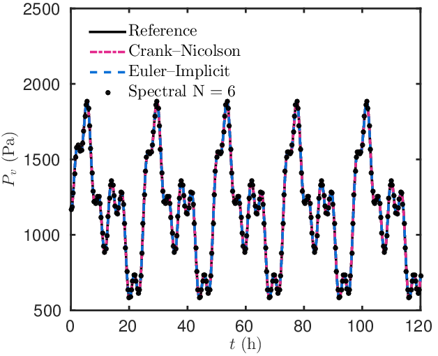
The absolute error $\varepsilon_{\,2}$ of the numerical methods applied and the reference solution is of the order of $\mathcal{O}\,(\,10^{\,-4}\,)\,$, as illustrated in Figure 3. The solutions of the problem have been computed for discretisation parameters of $\Delta x^{\,\star}\,=\,1\cdot 10^{\,-2}$ and $\Delta t^{\,\star}\,=\,1\cdot 10^{\,-1}$ for the Spectral–ROM and the Crank–Nicolson methods. However, the Euler implicit scheme needed more refinement to reach the same order of accuracy, with $\Delta x^{\,\star}\,=\,1\cdot 10^{\,-2}\text{ and }\Delta t^{\,\star}\,=\,1\cdot 10^{\,-2}\,$.

Figure 4(b) presents the absolute error $\varepsilon_{\,2}$ for the Spectral–ROM using different number of modes. As we increase the number of modes, the solution of the Spectral–ROM gets more accurate with the solution converging within few modes (less than 10). To illustrate the convergence of the solution, the profile of the vapour pressure for the last time instant of simulation is presented for a different number of modes in Figure 4(a). In this case, if we compare the solution with $3$ modes to the solution with $5$ modes a significant difference can be noticed. With $5$ modes we already have a satisfactory solution to the problem, with the absolute error of the order of $\mathcal{O}\,(\,10^{-3}\,)\,$, while the solution with $3$ modes is still oscillating. The number of modes of the Spectral method is predetermined in order to build the system of ODEs. In this case, a number of six modes proved to be good enough.

Spectral coefficients $a_{\,n}\,(\,t\,)$ are shown in Figures 5(a) and 5(b). It can be seen the first coefficients have the most significant values. For this reason, the Spectral method needs few modes to converge to the solution (an order of $10$) because its first modes have the highest magnitudes. A brief comparison with an analytical solution, built on Fourier decomposition [35], reveals that the eigenvalues of the Spectral method decrease faster, as shown in Figure 6. Note that the eigenvalues of the analytical solution do not have to coincide with the ones of the Spectral method since the eigenfunctions are not the same for the Chebyshev polynomials and the trigonometric ones. Furthermore, the magnitude of the last spectral coefficient acts as an error estimator, determining the error upper limit.

The global absolute error $\varepsilon_{\,\infty}$ for the conventional numerical methods applied is calculated as a function of spatial discretisation $\Delta x^{\,\star}\,$. Fig. 7 shows that the Spectral-ROM has the same accuracy for all values of $\Delta x^{\,\star}$. It is due to the fact that the Spectral method is based on Chebyshev polynomials, which enables to calculate the solution in each spatial node, as an analytical solution. For this reason, the error of the Spectral solution is almost a straight line, not depending on the spatial discretisation. However, for the conventional methods, the solution gets inaccurate when the value of $\Delta x^{\,\star}$ increases. It should be noted that the Spectral–ROM can provide even more accurate results, by increasing the number of modes or by decreasing the tolerance in the ODE Matlab solver to certain limits.

This case is called weakly nonlinear because the boundary conditions remain linear and, only the diffusion coefficient has a slight dependency on the moisture field. Thus, the diffusion equation is written as:

where, $\nu\,(\,u\,)\ =\ \nu_{\,0}\ +\ \nu_{\,1}\cdot u\,$. Since we have the diffusion coefficient depending on the field $\nu\,(\,u\,)$, the diffusion equation — Eq. (4.1) — can be rewritten as:

where the residual has the following form:

Then, by applying the Tau–Galerkin method, the residual is minimized by assuming it orthogonal to the basis functions $\langle\,R\,,\mathsf{T}_{\,k}\,\rangle\,=\,0\,$, which is defined in Eq. (3.6), leading to the following equation:

where,

Eq. (4.2) is a closed system of ODEs. Coefficients $c_{\,i,\,j,\,k}$ are calculated at once, and coefficient $\tilde{\tilde{a}}_{\,i}$ are related to $a_{\,i}$ though a linear transformation $\tilde{\tilde{a}}\ =\ \textsc{D}_{\,2}\cdot a$, in which $\textsc{D}_{\,2}\in\mathrm{Mat}\,_{(n-2)\times(n-2)}(\mathds{R})$ is a second order derivative matrix.

The number of operations for each approach can be estimated. We denote by $N_{\,x}$ and $N_{\,t}$ the number of nodes according to the discretisation in both space and time domains. For explicit methods, it can be related to the CFL type conditions. A standard approach based on the Euler implicit scheme requires $N_{\,x}\cdot N_{\,t}\,$, operations while the Crank–Nicolson scheme requires at least twice as many, as it is built on both implicit and explicit parts. Considering the same discretisation parameters $N_{\,t}\,=\,1200$ and $N_{\,x}\,=\,100$ for both methods, the number of operations for the linear case scales with:

Considering these discretisation parameters, the order of accuracy is not the same for both methods, it is at the order of $\varepsilon_{\infty}\simeq\mathcal{O}\,(10^{-3})$ for the Euler implicit and of $\varepsilon_{\infty}\simeq\mathcal{O}\,(10^{-4})$ for the Crank–Nicolson solution.

For the Spectral-ROM, the number is related to the solution of the system of ODEs (Eq. (3.8)), computed in this case with the Matlab solver ODE45. It is based on the iterative Runge–Kutta method to approximate the solution. The number of operation depends on the tolerance (tol) of the solver, which has a maximum tolerance of $\sim 10^{\,-5}$ for ODE45. Thus, we have:

where $\tau$ is the total time of simulation. At each time step, the Runge–Kutta needs to compute the vector product $\mathcal{A}_{\,s\times s}\,$, where $s$ depends on the degree of freedom $N$ of the solution ($s\,=\,N\,-\,2$). Thus, it leads to $6\cdot s^{\,2}$ operations to perform, knowing that $s$ is of the order of $10\,$. Consequently, the total number of operations for the Spectral-ROM scales with approximately:

Considering the first case, knowing that the tolerance was set to $10^{\,-4}\,$, with $N\,=\,6$ modes the number of operations performed by the Spectral–ROM is expressed by:

Comparing the number of operations of this case, we can already see that the Spectral–ROM is less costly than the other methods applied. Notice that the number of degrees of freedom necessary to solve the diffusion problem by means of the Spectral method is inferior to the ones necessary to solve the whole system of partial differential equations. Using Euler or Crank–Nicolson methods, the computational complexity scales with $p\,=\,N_{\,x}\,$, whereas the one Spectral–ROM is $s\,=\,(\,N\,-\,2\,)\,$. For this case, the numerical application gives $p\,\equiv\,10^{\,2}$ and $s\,\equiv\,4\,$. Moreover, we can note the reduction of the order of the solution, using the Spectral approach. According to the previous results, the fidelity of the model is not degraded but only the order of the solution. Besides, $N_{\,t}$ can not be reduced due to accuracy issues.

This case study considers moisture dependent coefficients $c_{\,m}$ and $d_{\,m}$, illustrated in Figures 12(a) and 12(b). Their variations are similar to the load bearing material from [22]. The initial vapour pressure is uniform $P_{\,v}^{\,i}\,=\,1.16\times 10^{\,\,3}$ $\mathsf{Pa}$. No moisture flow is taken into account at the boundaries. The ambient vapour pressures at the boundaries are illustrated in Figure 13. At the left boundary, it has a fast drop until the saturation state and at the right boundary, it has a sinusoidal variation. The material is thus excited until the capillary state. The convective vapour transfer coefficients are set to $h_{\,v,\,\mathrm{L}}\,=\,2\cdot 10^{\,-7}$ $\mathsf{s/m}$ and $h_{\,v,\,\mathrm{R}}\,=\,3\cdot 10^{\,-8}$ $\mathsf{s/m}$ for the left and right boundary, respectively. The simulation is performed for $120\,\mathsf{h}\,$. As in the previous case study, the dimensionless values can be found in Appendix A.

References

- [1] K. Abahri, R. Bennacer, and R. Belarbi. Sensitivity analyses of convective and diffusive driving potentials on combined heat air and mass transfer in hygroscopic materials. Numerical Heat Transfer, Part A: Applications, 69(10):1079–1091, may 2016.
- [2] M. Abuku, H. Janssen, and S. Roels. Impact of wind-driven rain on historic brick wall buildings in a moderately cold and humid climate: Numerical analyses of mould growth risk, indoor climate and energy consumption. Energy and Buildings, 41(1):101–110, jan 2009.
- [3] Z. Bai. Krylov subspace techniques for reduced-order modeling of large-scale dynamical systems. Appl. Numer. Math., 43(1-2):9–44, oct 2002.
- [4] E. Barreira, J. Delgado, N. Ramos, and V. Freitas. Hygrothermal Numerical Simulation: Application in Moisture Damage Prevention. In A. Lutz, editor, Numerical Simulations - Examples and Applications in Computational Fluid Dynamics, pages 567–578. InTech, Rijeka, nov 2010.
- [5] B. Bauklimatik Dresden. Simulation program for the calculation of coupled heat, moisture, air, pollutant, and salt transport. http://www.bauklimatik-dresden.de/delphin/index.php?aLa=en, 2011.
- [6] J. Berger, N. Mendes, S. Guernouti, M. Woloszyn, and F. Chinesta. Review of Reduced Order Models for Heat and Moisture Transfer in Building Physics with Emphasis in PGD Approaches. Archives of Computational Methods in Engineering, pages 1–13, jul 2016.
- [7] J. P. Boyd. Chebyshev and Fourier Spectral Methods. New York, 2nd edition, 2000.
- [8] D. M. Burch. An Analysis of Moisture Accumulation in Walls Subjected to Hot and Humid Climates. ASHRAE Transactions, 93(16):429–439, 1993.
- [9] C. Canuto, M. Y. Hussaini, A. Quarteroni, and T. A. Zang. Spectral Methods Fundamentals in Single Domains. Scientific Computation. Springer-Verlag Berlin Heidelberg, 2006.
- [10] S.-S. Chen, B.-W. Li, and Y.-S. Sun. Chebyshev collocation spectral method for solving radiative transfer with the modified discrete ordinates formulations. Int. J. Heat Mass Transfer, 88:388–397, sep 2015.
- [11] Y.-Y. Chen, B.-W. Li, and J.-K. Zhang. Spectral collocation method for natural convection in a square porous cavity with local thermal equilibrium and non-equilibrium models. Int. J. Heat Mass Transfer, 96:84–96, may 2016.
- [12] A. Dalgliesh, S. Cornick, W. Maref, and P. Mukhopadhyaya. Hygrothermal Performance of Building Envelopes: Uses for 2D and 1D simulation. In 10th Conference on Building Science and Technology, Ottawa, Canada, 2005. NRC Publication Archive.
- [13] V. P. De Freitas, V. Abrantes, and P. Crausse. Moisture migration in building walls - Analysis of the interface phenomena. Building and Environment, 31(2):99–108, mar 1996.
- [14] G. H. Dos Santos and N. Mendes. Simultaneous heat and moisture transfer in soils combined with building simulation. Energy and Buildings, 38(4):303–314, 2006.
- [15] T. A. Driscoll, N. Hale, and L. N. Trefethen. Chebfun Guide. Pafnuty Publications, Oxford, 2014.
- [16] I. Fraunhofer. Wufi. http://www.hoki.ibp.fhg.de/wufi/wufi_frame_e.html, 2005.
- [17] S. Gasparin, J. Berger, D. Dutykh, and N. Mendes. Stable explicit schemes for simulation of nonlinear moisture transfer in porous materials. J. Building Perf. Simul., 11(2):129–144, 2018.
- [18] W. Gautschi. Orthogonal Polynomials: Computation and Approximation. Oxford University Press, Oxford, UK, 2004.
- [19] W. Guo, G. Labrosse, and R. Narayanan. The Application of the Chebyshev-Spectral Method in Transport Phenomena, volume 68 of Lecture Notes in Applied and Computational Mechanics. Springer Berlin Heidelberg, Berlin, Heidelberg, 2012.
- [20] C.-E. Hagentoft, A. S. Kalagasidis, B. Adl-Zarrabi, S. Roels, J. Carmeliet, H. Hens, J. Grunewald, M. Funk, R. Becker, D. Shamir, O. Adan, H. Brocken, K. Kumaran, and R. Djebbar. Assessment Method of Numerical Prediction Models for Combined Heat, Air and Moisture Transfer in Building Components: Benchmarks for One-dimensional Cases. J. Building Phys., 27(4):327–352, apr 2004.
- [21] C. Herzet, P. Héas, and A. Drémeau. Model reduction from partial observations. Int. J. Num. Meth. in Eng., 113(3):479–511, jan 2018.
- [22] H. Janssen. Simulation efficiency and accuracy of different moisture transfer potentials. J. Building Perf. Simul., 7(5):379–389, sep 2014.
- [23] H. Janssen, B. Blocken, and J. Carmeliet. Conservative modelling of the moisture and heat transfer in building components under atmospheric excitation. Int. J. Heat Mass Transfer, 50(5-6):1128–1140, mar 2007.
- [24] B.-W. Li, Y.-S. Sun, and Y. Yu. Iterative and direct Chebyshev collocation spectral methods for one-dimensional radiative heat transfer. Int. J. Heat Mass Transfer, 51(25-26):5887–5894, dec 2008.
- [25] W. Liu, J. Sun, and B. Wu. Galerkin-Chebyshev spectral method and block boundary value methods for two-dimensional semilinear parabolic equations. Numerical Algorithms, 71(2):437–455, feb 2016.
- [26] D. J. Lucia, P. S. Beran, and W. A. Silva. Reduced-order modeling: new approaches for computational physics. Progress in Aerospace Sciences, 40(1-2):51–117, feb 2004.
- [27] A. V. Luikov. Heat and mass transfer in capillary-porous bodies. Pergamon Press, New York, 1966.
- [28] H. Ma, Y. Qin, and Q. Ou. Multidomain Legendre-Galerkin Chebyshev-collocation method for one-dimensional evolution equations with discontinuity. Applied Numerical Mathematics, 111(Supplement C):246–259, jan 2017.
- [29] J. Ma, B.-W. Li, and J. R. Howell. Thermal radiation heat transfer in one- and two-dimensional enclosures using the spectral collocation method with full spectrum k-distribution model. International Journal of Heat and Mass Transfer, 71:35–43, apr 2014.
- [30] N. Mendes, M. Chhay, J. Berger, and D. Dutykh. Numerical methods for diffusion phenomena in building physics. PUCPRess, Curitiba, Parana, 2017.
- [31] N. Mendes and P. C. Philippi. A method for predicting heat and moisture transfer through multilayered walls based on temperature and moisture content gradients. Int. J. Heat Mass Transfer, 48(1):37–51, 2005.
- [32] N. Mendes, I. Ridley, R. Lamberts, P. C. Philippi, and K. Budag. Umidus: A PC program for the Prediction of Heat and Mass Transfer in Porous Building Elements. In IBPSA 99, pages 277–283, Japan, 1999. International Conference on Building Performance Simulation.
- [33] L. H. Mortensen, M. Woloszyn, C. Rode, and R. Peuhkuri. Investigation of Microclimate by CFD Modeling of Moisture Interactions between Air and Constructions. J. Building Phys., 30(4):279–315, apr 2007.
- [34] S. Motsa. On the New Bivariate Local Linearisation Method for Solving Coupled Partial Differential Equations in Some Applications of Unsteady Fluid Flows with Heat and Mass Transfer. In M. Solecki, editor, Mass Transfer - Advancement in Process Modelling. InTech, Rijeka, oct 2015.
- [35] M. N. Ozisik. Heat conduction. Wiley-Interscience, New York, 2 edition, 1993.
- [36] A. Pasban, H. Sadrnia, M. Mohebbi, and S. A. Shahidi. Spectral method for simulating 3D heat and mass transfer during drying of apple slices. Journal of Food Engineering, 212(Supplement C):201–212, nov 2017.
- [37] R. Peyret. Spectral methods for incompressible viscous flow. Springer-Verlag, New York, 2002.
- [38] PUCPR. Domus. http://www.domus.pucpr.br/, (Pontifical Catholic University of Parana), 2018.
- [39] C. RamReddy, P. A. Lakshmi Narayana, and S. S. Motsa. A spectral relaxation method for linear and non-linear stratification effects on mixed convection in a porous medium. Appl. Math. Comput., 268:991–1000, oct 2015.
- [40] S. R. Reddy, B. A. Freno, P. G. A. Cizmas, S. Gokaltun, D. McDaniel, and G. S. Dulikravich. Constrained reduced-order models based on proper orthogonal decomposition. Computer Methods in Applied Mechanics and Engineering, 321:18–34, jul 2017.
- [41] C. Rode and K. Grau. Whole Building Hygrothermal Simulation Model. ASHRAE Transactions, 109(1):572–582, 2003.
- [42] S. Rouchier, M. Woloszyn, G. Foray, and J.-J. Roux. Influence of concrete fracture on the rain infiltration and thermal performance of building facades. Int. J. Heat Mass Transfer, 61:340–352, jun 2013.
- [43] W. Schilders. Introduction to Model Order Reduction. In W. H. A. Schilders, H. A. van der Vorst, and J. Rommes, editors, Model Order Reduction: Theory, Research Aspects and Applications, pages 3–32. Springer, Berlin, Heidelberg, 2008.
- [44] L. F. Shampine and M. W. Reichelt. The MATLAB ODE Suite. SIAM J. Sci. Comput., 18:1–22, 1997.
- [45] G. Stabile and G. Rozza. Finite volume POD-Galerkin stabilised reduced order methods for the parametrised incompressible Navier-Stokes equations. Computers & Fluids, feb 2018.
- [46] H.-J. Steeman, M. Van Belleghem, A. Janssens, and M. De Paepe. Coupled simulation of heat and moisture transport in air and porous materials for the assessment of moisture related damage. Building and Environment, 44(10):2176–2184, oct 2009.
- [47] L. N. Trefethen. Finite Difference and Spectral Methods for Ordinary and Partial Differential Equations. Unpublished, Ithaca, NY, USA, 1996.
- [48] L. N. Trefethen. Spectral methods in MatLab. Society for Industrial and Applied Mathematics, Philadelphia, PA, USA, 2000.
- [49] S. Ullmann, M. Rotkvic, and J. Lang. POD-Galerkin reduced-order modeling with adaptive finite element snapshots. J. Comp. Phys., 325:244–258, nov 2016.
- [50] C. Wang, Z. Qiu, and Y. Yang. Collocation methods for uncertain heat convection-diffusion problem with interval input parameters. Int. J. Therm. Sci., 107:230–236, sep 2016.
- [51] M. Woloszyn and C. Rode. Tools for performance simulation of heat, air and moisture conditions of whole buildings. Building Simulation, 1(1):5–24, mar 2008.