跳到论文正文
W Papers独立论文阅读器 arXiv:1704.07334 论文正文 计算阅读时间 · 0%
引用这篇论文根据当前论文元数据生成,正式投稿前建议核对。


License: arXiv.org perpetual non-exclusive license
arXiv:1704.07334v3 [cond-mat.other] 18 Jun 2017

Universal linear and nonlinear electrodynamics of the Dirac fluid

Zhiyuan Sun Affiliation: Department of Physics, University of California San Diego, 9500 Gilman Drive, La Jolla, California 92093, USA    D. N. Basov Affiliation: Department of Physics, University of California San Diego, 9500 Gilman Drive, La Jolla, California 92093, USA Affiliation: Department of Physics, Columbia University, 538 West 120th Street, New York, New York 10027    M. M. Fogler Affiliation: Department of Physics, University of California San Diego, 9500 Gilman Drive, La Jolla, California 92093, USA
August 24, 2026
Abstract

A general relation is derived between the linear and second-order nonlinear ac conductivities of an electron system in the hydrodynamic regime of frequencies below the interparticle scattering rate. The magnitude and tensorial structure of the hydrodynamic nonlinear conductivity are shown to differ from their counterparts in the more familiar kinetic regime of higher frequencies. Due to universality of the hydrodynamic equations, the obtained formulas are valid for systems with an arbitrary Dirac-like dispersion, ranging from solid-state electron gases to free-space plasmas, either massive or massless, at any temperature, chemical potential or space dimension. Predictions for photon drag and second-harmonic generation in graphene are presented as one application of this theory.

There has been a renewed interest to hydrodynamic phenomena in electron systems with a Dirac-like energy-momentum dispersion εp2=(p​v)2+(m​v2)2\varepsilon_{p}^{2}=(pv)^{2}+(mv^{2})^{2}. This subject was revived by studies in quantum criticality and holographic field theory [1] and outspread in research on two-dimensional (2D) conductors, e.g., graphene where the massless dispersion m=0m=0 is realized [2, 3, 4, 5, 6, 7, 8, 9, 10, 11, 12, 13, 14]. An experimental observation of a viscous electron flow in graphene has been recently reported [9]. Although not uncommon in plasmas [15], this type of transport is highly unusual in a solids. It may be possible only in a limited range of temperatures TT and chemical potentials μ\mu in pristine samples where the combined rate of electron-impurity (ei) and electrons-phonon (ep) scattering Γd=Γe​i+Γe​p\Gamma_{d}=\Gamma_{ei}+\Gamma_{ep} is lower than the momentum-conserving electron-electron (ee) scattering rate Γe​e\Gamma_{ee} [16, 17]. The respective mean-free paths must obey the inequality ld≫le​el_{d}\gg l_{ee}. Under these conditions, the electron dynamics at frequencies ω≪Γe​e\omega\ll\Gamma_{ee} and momenta q≪le​e−1q\ll l_{ee}^{-1} is governed by collective variables that obey hydrodynamic equations [18]. The frequency range Γd<ω<Γe​e\Gamma_{d}<\omega<\Gamma_{ee} may be as wide as several THz in graphene (see below). Therefore exploring electrodynamics of Dirac fluids may be worthwhile.

In this Letter we focus on the second-order ac conductivity, which controls nonlinear optical phenomena such as sum (difference) frequency generation and also photon drag. In the Supplemental material [19], we also discuss the third-order conductivity important for the Kerr effect. Prior work [20, 21, 22, 23, 24, 25, 26, 27, 28] has indicated that in graphene such effects may or may not [29] be stronger than in typical metals and semiconductors. We find significant differences of our results from what one obtains at frequencies ω>Γe​e\omega>\Gamma_{ee} where the dynamics is described by the Boltzmann kinetic equation. The still higher frequency quantum regime (Fig. 1) is beyond the scope of our investigation.

Refer to caption
Figure 1: A sketch of hydrodynamic, kinetic, and quantum domains in the frequency-momentum space. The collective modes of a massless fluid (plasmons and demons) are also shown, see text.

Recall that the second-order conductivity is a third-rank tensor σi​l​m(2)​(𝐪1,ω1,𝐪2,ω2)\sigma^{(2)}_{ilm}\left(\mathbf{q}_{1},\omega_{1};\mathbf{q}_{2},\omega_{2}\right) that describes the current of frequency ω3=ω1+ω2\omega_{3}=\omega_{1}+\omega_{2} and momentum 𝐪3=𝐪1+𝐪2\mathbf{q}_{3}=\mathbf{q}_{1}+\mathbf{q}_{2} generated, to the order O⁡(𝐄2){O}\left(\mathbf{E}^{2}\right), in response to an electric field

𝐄⁡(𝐫,t)=𝐄⁡(𝐪1,ω1)​ei​𝐪1​𝐫−i​ω1​t+𝐄⁡(𝐪2,ω2)​ei​𝐪2​𝐫−i​ω2​t+c.c.\mathbf{E}(\mathbf{r},t)=\mathbf{E}(\mathbf{q}_{1},\omega_{1})e^{i\mathbf{q}_{1}\mathbf{r}-i\omega_{1}t}+\mathbf{E}(\mathbf{q}_{2},\omega_{2})e^{i\mathbf{q}_{2}\mathbf{r}-i\omega_{2}t}+\mathrm{c.c.} (1)

By convention, σi​l​m(2)\sigma^{(2)}_{ilm} is symmetrized, i.e., invariant under the interchange (1↔2,l↔m)(1\leftrightarrow 2,l\leftrightarrow m). If the system preserves parity, which we assume to be the case, σi​l​m(2)\sigma^{(2)}_{ilm} must vanish if both 𝐪ν\mathbf{q}_{\nu}, ν=1,2\nu=1,2 are zero. At small 𝐪ν\mathbf{q}_{\nu}, relevant for optical/THz experiments, σi​l​m(2)\sigma^{(2)}_{ilm} should scale linearly with 𝐪ν\mathbf{q}_{\nu}. In comparison, dissipative effects due to viscosity and heat conduction [17, 30], which scale as |𝐪ν|2|\mathbf{q}_{\nu}|^{2}, are subleading: the fluid dynamics is approximately isentropic (ise) [18]. Below we show that in this regime the second-order conductivity has the universal form

σi​l​m(2)=Dh(2)ω1​ω2​ω3​(ω3ω1​q1​l​δi​m+q1​i​δl​m)+(1↔2l↔m),\sigma^{(2)}_{ilm}=\frac{D_{h}^{(2)}}{\omega_{1}\omega_{2}\omega_{3}}\left(\frac{\omega_{3}}{\omega_{1}}q_{1l}\delta_{im}+q_{1i}\delta_{lm}\right)+\left(\begin{smallmatrix}1&\leftrightarrow&2\\ l&\leftrightarrow&m\end{smallmatrix}\right)\,, (2)

for an arbitrary mass mm, equilibrium charge density ρ\rho, temperature TT, and space dimension dd. All the material-specific parameters are contained in the second-order spectral weight Dh(2)D_{h}^{(2)}, which we find to be equal to the derivative

Dh(2)=−14​π2​(∂(Dh)2∂ρ)iseD_{h}^{(2)}=-\frac{1}{4\pi^{2}}\left(\frac{\partial(D_{h})^{2}}{\partial\rho}\right)_{\mathrm{ise}} (3)

of the squared linear-response (i.e., Drude) spectral weight

Dh=π​e2​nm∗,n≡ρe.D_{h}=\pi\,\frac{e^{2}n}{m^{\ast}}\,,\quad n\equiv\frac{\rho}{e}\,. (4)

As stated above, these formulas hold for either massless or massive electrons. Conventional metals and semiconductors have a parabolic dispersion. This case is exemplified by the nonrelativistic limit |μ|,T≪m​v2|\mu|,T\ll mv^{2} of our equations, yielding m∗=mm^{\ast}=m. This result can also be understood as the consequence of Galilean invariance, which demands that the ee interactions affect the linear and nonlinear conductivities only in higher orders in 𝐪ν\mathbf{q}_{\nu}. This is why the effective mass m∗m^{\ast} in Eq. (S2) is equal to the bare mass mm and the leading 𝐪ν\mathbf{q}_{\nu}-linear terms of σi​l​m(2)\sigma^{(2)}_{ilm} [Eq. (2)] are the same in hydrodynamic [15], kinetic [31], and quantum [32] domains. The equality of m∗m^{*} and mm does not hold if either |μ||\mu| or TT are comparable or larger than the energy gap 2​m​v22mv^{2}, e.g., in the case of graphene. (For linear conductivity at T=0T=0 this has been discussed at length [33, 34, 35].)

In the hydrodynamic regime of graphene, frequent collisions force electrons and holes to move together, causing cancellation of their partial currents. This enhances m∗m^{\ast} and reduces DhD_{h} below its kinetic counterpart DkD_{k} at all T>0T>0, see Fig. 2(a). Similarly, Dh(2)D_{h}^{(2)} decreases with TT at fixed ρ\rho much faster in the hydrodynamic regime than in the previously studied kinetic one, see Fig. 2(b).

Refer to caption
Figure 2: (Color online) (a) Hydrodynamic DhD_{h} and kinetic DkD_{k} Drude weights of doped graphene as functions of TT, normalized to their common T=0T=0 value. The dashed lines are sketches of the effective Drude weight π​ω​Im​[σ⁡(ω)]\pi\omega\mathrm{Im}[\sigma(\omega)] at three different frequencies ω∼εF\omega\sim\varepsilon_{F} marked 11–33 from low to high. (b) The second-order spectral weights Dk(2)D_{k}^{(2)} and Dh(2)D_{h}^{(2)} of graphene in units of D0(2)D_{0}^{(2)}, Eq. (11). The Fermi energy εF=0.207​eV\varepsilon_{F}=0.207\,\mathrm{eV} in both panels, corresponding to n=3.14×10¹²​cm−2n=3.14\times 10^{12}\,\mathrm{cm^{-2}}.

Let us now present a qualitative argument for Eq. (2). Consider the expansion of a given Fourier harmonic of the electric current ji​(𝐪,ω)=ji(1)​(𝐪,ω)+ji(2)​(𝐪,ω)+…j_{i}(\mathbf{q},\omega)=j_{i}^{(1)}(\mathbf{q},\omega)+j_{i}^{(2)}(\mathbf{q},\omega)+\ldots in power series of the driving electric field 𝐄\mathbf{E}. The first term is given by ji(1)​(𝐪,ω)=σi​j​(𝐪,ω)​Fi(1)​(𝐪,ω)j_{i}^{(1)}(\mathbf{q},\omega)=\sigma_{ij}(\mathbf{q},\omega)F_{i}^{(1)}(\mathbf{q},\omega) where Fi(1)​(𝐪,ω)=Ei​(𝐪,ω)+𝒪⁡(𝐪)F_{i}^{(1)}(\mathbf{q},\omega)=E_{i}(\mathbf{q},\omega)+\mathcal{O}(\mathbf{q}) is the driving force per unit charge and σi​j\sigma_{ij} is the linear-response conductivity tensor. It suffices to consider the 𝐪→0\mathbf{q}\to 0 limit in which Fi(1)→EiF_{i}^{(1)}\to E_{i}, σi​j→δi​j​σ\sigma_{ij}\to\delta_{ij}\sigma. The scalar σ\sigma can be in general separated into the Drude pole and a nonsingular correction σ0\sigma_{0} (to be discussed below):

σ⁡(q=0,ω)=1π​Dh−i​ω+Γd+σ0,ω≪Γe​e.\displaystyle\sigma(q=0,\omega)=\frac{1}{\pi}\,\frac{D_{h}}{-i\omega+\Gamma_{d}}+\sigma_{0}\,,\quad\omega\ll\Gamma_{ee}\,. (5)

Next, to the second order we expect ji(2)=σ(1)​Fi(1)+σ​Fi(2)j_{i}^{(2)}=\sigma^{(1)}F_{i}^{(1)}+\sigma F_{i}^{(2)}. Here σ(1)=(∂σ/∂ρ)​ρ(1)\sigma^{(1)}=(\partial\sigma/\partial\rho)\rho^{(1)} and ρ(1)\rho^{(1)} are the perturbations of the conductivity and charge density. The latter perturbation can be found from the continuity equation (S23a), which gives ρ(1)​(𝐪,ω)=𝐪⋅𝐣(1)​(𝐪,ω)/ω\rho^{(1)}(\mathbf{q},\omega)=\mathbf{q}\cdot\mathbf{j}^{(1)}(\mathbf{q},\omega)/\omega. Calculation of the second-order driving force Fi(2)F_{i}^{(2)} is the difficult part of the problem. We glean the answer from the ω1≃−ω2≫ω3\omega_{1}\simeq-\omega_{2}\gg\omega_{3} case where it is equal to the sum of the pondermotive and Abraham forces [36]. The former is of order (ω3)0(\omega_{3})^{0}, the latter is the leading (ω3)1(\omega_{3})^{1} correction. Following [36], Sec. 81, we find the real-space representation of the pondermotive force to be

Fi(2)​(𝐫)=i2​∂i[𝐄⁡(𝐫,ω1)ω2​∂σ⁡(ω2)∂ρ​𝐄​(𝐫,ω2)+(1↔2)]=−i2∂i[𝐄⁡(𝐫,ω1)ω1∂σ⁡(ω2)∂ρ𝐄(𝐫,ω2)+(1↔2)].\begin{split}F^{(2)}_{i}(\mathbf{r})&=\frac{i}{2}\,\partial_{i}\left[\frac{\mathbf{E}(\mathbf{r},\omega_{1})}{\omega_{2}}\frac{\partial\sigma(\omega_{2})}{\partial\rho}\mathbf{E}(\mathbf{r},\omega_{2})+(1\leftrightarrow 2)\right]\\ &=-\frac{i}{2}\,\partial_{i}\left[\frac{\mathbf{E}(\mathbf{r},\omega_{1})}{\omega_{1}}\frac{\partial\sigma(\omega_{2})}{\partial\rho}\mathbf{E}(\mathbf{r},\omega_{2})+(1\leftrightarrow 2)\right].\end{split} (6)

The replacement of ω2\omega_{2} by −ω1-\omega_{1} in the second line cannot be strictly justified if ω3≠0\omega_{3}\neq 0. However, it is a natural way to ensure the triangular permutation symmetry of σi​l​m(2)\sigma^{(2)}_{ilm}, which follows from the energy conservation [37] in the dissipationless limit Γd,σ0→0\Gamma_{d},\sigma_{0}\to 0. Assembling all the terms of ji(2)j_{i}^{(2)}, we can read off σi​l​m(2)\sigma^{(2)}_{ilm} and see it coincides with Eq. (2). One can verify that for a nonrelativistic electron gas our formulas agree with those in literature [15, 31].

The case of a Lorentz-invariant Dirac fluid can be studied rigorously. Proposed solid-state examples of such fluids [1] actually lack true Lorentz invariance. Their matter and field components have different limiting velocities, vv and cc. However, if Coulomb interactions are weak, the approximate Lorentz invariance with velocity vv holds. In graphene this is so if the dielectric constant κ\kappa of the environment is large, so that the interaction constant e2/(ℏ​κ​v)e^{2}/(\hbar\kappa v) is small. We will use relativistic hydrodynamics to derive DhD_{h} and Dh(2)D_{h}^{(2)} for this model and verify our key result (2).

Let us introduce two additional quanitites. One is the flow velocity 𝐮\mathbf{u} that defines the electric current 𝐣=ρ​𝐮\mathbf{j}=\rho\mathbf{u}. The other is the energy density nE=γ2​W−Pn_{E}=\gamma^{2}W-P related to the pressure P=P⁡(μ,T)P=P(\mu,T) and enthalpy density W=W⁡(μ,T)W=W(\mu,T) at thermal equilibrium, u=0u=0 [18]. Here γ≡1/1−(u/v)2\gamma\equiv{1}/\sqrt{1-(u/v)^{2}} and nEn_{E} is referenced to the μ=T=u=0\mu=T=u=0 state. Relativistic hydrodynamic equations admit many equivalent formulations [18, 3, 4, 38, 5], e.g.,

∂tρ+div⁡1​𝐣=0,\displaystyle\partial_{t}\rho+\div 1\mathbf{j}=0\,, (7a)
∂tnE+div⁡1​(γ2​W​𝐮)=𝐣⋅𝐄,\displaystyle\partial_{t}n_{E}+\div 1\left(\gamma^{2}W\mathbf{u}\right)=\mathbf{j}\cdot\mathbf{E}\,, (7b)
(γ2​m∗​n)​𝒟t​𝐮=ρ​𝐅L−𝐮v2​(𝐣⋅𝐄)−𝒟​P,\displaystyle(\gamma^{2}m^{\ast}\!n)\,\mathcal{D}_{t}\mathbf{u}=\rho\mathbf{F}_{L}-\frac{\mathbf{u}}{v^{2}}\left(\mathbf{j}\cdot\mathbf{E}\right)-\mathbf{\mathcal{D}}P\,, (7c)
m∗=Wn​v2,𝐅L=𝐄+1c𝐮×𝐁,curl𝐄=−1c∂t𝐁.\displaystyle m^{\ast}=\frac{W}{nv^{2}}\,,\quad\mathbf{F}_{L}=\mathbf{E}+\frac{1}{c}\,\mathbf{u}\times\mathbf{B}\,,\quad\curl\mathbf{E}=-\frac{1}{c}\partial_{t}\mathbf{B}\,. (7d)

The first pair is the charge continuity equation and the energy conservation equation sans the subleading viscous and thermal conductivity terms. Equation (7d) for the Lorentz force 𝐅L\mathbf{F}_{L} includes the force from the ac magnetic field 𝐁\mathbf{B} induced by 𝐄\mathbf{E}. (We assume that no static magnetic field is present.) This term is important if 𝐄\mathbf{E}-field has a transverse component. Equation (S23c) is the relativistic Euler equation written in “covariant derivatives” 𝒟i=∂i+(ui/v2)∂t\mathcal{D}_{i}=\partial_{i}+({u}_{i}/{v^{2}})\partial_{t}, 𝒟t=∂t+Γd+ui∂i\mathcal{D}_{t}=\partial_{t}+\Gamma_{d}+{u}_{i}\partial_{i} with the scattering rate Γd\Gamma_{d} accounting for momentum dissipation. We solve these equations for 𝐣\mathbf{j} perturbatively in 𝐄\mathbf{E} to get the desired conductivities.

The linear response has already been treated at length [1, 3, 4, 38, 5, 6, 12, 13]. For massless particles, W=(d+1)​P=d+1d​nE∝Td+1W=(d+1)P=\frac{d+1}{d}n_{E}\propto T^{d+1}. The hydrodynamic Drude weight Dh=π​ρ2​v2/WD_{h}=\pi\rho^{2}v^{2}/W [cf. Eqs. (S2) and (7d)] decreases as T−d−1T^{-d-1} with TT, i.e., as T−3T^{-3} in graphene. The usual, kinetic Drude weight Dk​(μ,T)=(g/2)​(e/ℏ)2​T​ln⁡[2​cosh⁡(μ/2​T)]D_{k}(\mu,T)=(g/2)({e}/{\hbar})^{2}T\ln\left[2\cosh({\mu}/{2T})\right] where g=4g=4 is the number of Dirac cones [34] behaves differently. After some initial drop, DkD_{k} increases with TT because of thermal excitation of carriers, see Fig. 2(a). The question how the opposite trends of DhD_{h} and DkD_{k} could be reconciled has not been given proper attention in prior literature. As a tentative answer, we suggest the interpolation formula:

σ⁡(q=0,ω)\displaystyle\sigma(q=0,\omega) =1π​Dh−i​ω+Γd+1π​Dk−Dh−i​ω+Γd+Γe​e.\displaystyle=\frac{1}{\pi}\frac{D_{h}}{-i\omega+\Gamma_{d}}+\frac{1}{\pi}\frac{D_{k}-D_{h}}{-i\omega+\Gamma_{d}+\Gamma_{ee}}\,. (8)

This formula can be derived from the Boltzmann kinetic equation with the ee scattering rate Γe​e\Gamma_{ee} added to the collision integral [19]. Matching it with Eq. (5) at ω≪Γe​e\omega\ll\Gamma_{ee}, we deduce the parameter σ0=(Dk−Dh)/(π​Γe​e)\sigma_{0}=(D_{k}-D_{h})/(\pi\Gamma_{ee}) therein (we assume Γd≪Γe​e\Gamma_{d}\ll\Gamma_{ee}) [5]. According to Eq. (S17), the effective Drude weight π​ω​Im⁡σ\pi\omega\im\sigma as a function of ω\omega exhibits two plateaus, see Fig. 3, and σ\sigma as a function of TT at fixed ω\omega may look like as sketched in Fig. 2(a). A quantitative theory of these crossover behaviors is a challenge for future work. Meanwhile, Fig. 3 indicates the existence of two separate frequency intervals where Im⁡σ⁡(ω)≫Re⁡σ⁡(ω)\im\sigma(\omega)\gg\re\sigma(\omega). In these intervals weakly damped collective modes are possible: sound waves [38] (or energy waves [39] or “demons” [12] ) in the hydrodynamic regime and plasmons in the kinetic one, see also Fig. 1.

Refer to caption
Figure 3: (Color online) Schematic illustration of Eq. (S17). The black curve is the effective Drude weight π​ω​Im⁡σ\pi\omega\im\sigma as a function of ω\omega at fixed ρ\rho and TT. The red curve represents π​ω​Re⁡σ\pi\omega\re\sigma and ω\omega should be understood as plotted on a logarithmic scale. The insets depict collective motion of electrons and holes in plasmons and demons.

Let us move on to the second-order conductivity, ignoring the momentum dissipation for now, Γd→0\Gamma_{d}\to 0. In the hydrodynamic regime we have two ways to derive σi​l​m(2)\sigma^{(2)}_{ilm}. The quick one is via Eq. (2). The only unknown parameter is Dh(2)D_{h}^{(2)}, which we can calculate from Eq. (3) applied to Dh=π​ρ2​v2/WD_{h}=\pi\rho^{2}v^{2}/W. This yields

Dh(2)=−12​e3​nm∗2​(1−Cise),\displaystyle D_{h}^{(2)}=-\frac{1}{2}\frac{e^{3}n}{m^{\ast 2}}(1-C_{\mathrm{ise}})\,, (9)

where

Cise=nW​(∂P∂n)ise=1m∗​v2​(∂P∂n)ise\displaystyle C_{\mathrm{ise}}=\frac{n}{W}\left(\frac{\partial P}{\partial n}\right)_{\mathrm{ise}}=\frac{1}{m^{\ast}\!v^{2}}\left(\frac{\partial P}{\partial n}\right)_{\mathrm{ise}} (10)

is the dimensionless isentropic bulk modulus. Note that for massless electrons Cise=1/dC_{\mathrm{ise}}=1/d. The second derivation we can do is from hydrodynamic Eqs. (S23), which is more tedious [19] but gives the same result. This verifies the validity of our universal formula (2) for Dirac fluids.

Let us examine the TT-dependence of the spectral weight Dh(2)D_{h}^{(2)}. As one can anticipate, Dh(2)D_{h}^{(2)} rapidly decreases at high TT, e.g., Dh(2)∝T−2​d−2=T−6D_{h}^{(2)}\propto T^{-2d-2}=T^{-6} for graphene. At T→0T\to 0, Eq. (9) predicts Dh(2)→2​D0(2)​sign​nD_{h}^{(2)}\to 2D_{0}^{(2)}\mathrm{sign}\,n, where

D0(2)=−g32​π​e3​v2ℏ2.\displaystyle D_{0}^{(2)}=-\frac{g}{32\pi}\frac{e^{3}v^{2}}{\hbar^{2}}\,. (11)

It may seem unusual that Dh(2)D_{h}^{(2)} becomes doping-independent in this limit (except for the overall sign) but this can be rationalized by the dimensional analysis. Of course, at T=0T=0 the system must be in the kinetic not hydrodynamic regime. Surprisingly, in the kinetic regime of graphene, σi​l​m(2)\sigma^{(2)}_{ilm} has a different tensorial structure:

σi​l​m(2)=\displaystyle\sigma^{(2)}_{ilm}=\mbox{} Dk(2)ω1​ω2​ω3​Σi​l​m​n​(ω1,ω2)​q1​n+(1↔2l↔m),\displaystyle\frac{D^{(2)}_{k}}{\omega_{1}\omega_{2}\omega_{3}}\,\Sigma_{ilmn}(\omega_{1},\omega_{2})q_{1n}+\left(\begin{smallmatrix}1&\leftrightarrow&2\\ l&\leftrightarrow&m\end{smallmatrix}\right)\,, (12)
Σi​l​m​n=−(1−3​ω3ω1)​δi​m​δn​l−(1+ω3ω1)​δi​l​δn​m+(3−ω3ω1)​δi​n​δl​m.\displaystyle\begin{split}\Sigma_{ilmn}=&-\left(1-3\,\frac{\omega_{3}}{\omega_{1}}\right)\delta_{im}\delta_{nl}-\left(1+\frac{\omega_{3}}{\omega_{1}}\right)\delta_{il}\delta_{nm}\\ &\mbox{}+\left(3-\frac{\omega_{3}}{\omega_{1}}\right)\delta_{in}\delta_{lm}\,.\end{split} (13)

This result can be obtained from either the Boltzmann kinetic equation [27] or the semiclassical limit q≪kFq\ll k_{F}, ω≪εF\omega\ll\varepsilon_{F} of the quantum random-phase approximation [26, 24, 28]. Here εF\varepsilon_{F} and kFk_{F} are the Fermi energy and momentum. Note that some of the related formulas in prior literature, e.g., Eq. (A.8) of [27] and Eq. (42) of [28] are valid only for response to a longitudinal 𝐄\mathbf{E}-field. If curl⁡𝐄≠0\curl\mathbf{E}\neq 0, the correct result is obtained only if the induced 𝐁\mathbf{B}-field is included [26, 24, 19]. When extended further [19], such calculations show that Dk(2)=D0(2)D^{(2)}_{k}=D_{0}^{(2)} at T=0T=0 and Dk(2)∝T−2D^{(2)}_{k}\propto T^{-2} at high TT. Hence, Dh(2)D_{h}^{(2)} is twice larger than Dk(2)D_{k}^{(2)} at T=0T=0 but becomes smaller at high TT, see Fig. 2(b).

Refer to caption
Figure 4: (Color online) (a) Geometry for measuring PD, second, and third harmonic generation. (b) SHG signal as a function of TT at fixed ω\omega. The “Kinetic” curve is from Eq. (2); the “Hydro” curve is from Eq. (12); the dashed curve is a sketch of the actual signal. (c) PD photocurrent jxj_{x} in graphene vs. polarization angle α\alpha (illustrated by the red arrows). (d) jyj_{y} vs. phase delay ψ\psi (degree of circular polarization) at α=π/4\alpha=\pi/4. Parameters in (c,d): T=0T=0 for the ‘Kinetic” curves, T=300​KT=300\,\mathrm{K} for the “Hydro” curves, n=3.14×10¹²​cm−2n=3.14\times 10^{12}\,\mathrm{cm^{-2}}, ω=5​THz\omega=5\,\mathrm{THz}, Γd=1​THz\Gamma_{d}=1\,\mathrm{THz}, θ=π/4\theta=\pi/4, E=103​V/cmE=10^{3}\,\mathrm{V/cm}.

A direct experimental probe of the second-order spectral weight is the second harmonic generation (SHG), which corresponds to ω2=ω1=ω\omega_{2}=\omega_{1}=\omega, ω3=2​ω\omega_{3}=2\omega, see Fig. S2(a). As explained above, the hydrodynamics predicts the SHG signal that is twice larger at low TT and much smaller at high TT compared to the standard kinetic theory [21, 23], see Fig. S2(b). The crossover from the kinetic regime to the hydrodynamic one would occur at temperature T∗T^{\ast} such that Γe​e​(T∗)=ω\Gamma_{ee}\left(T^{\ast}\right)=\omega. The measured SHG signal may look like as sketched by the dashed curve in Fig. S2(b).

Another effect controlled by σi​l​m(2)\sigma^{(2)}_{ilm} is the photon drag (PD), the generation of a dc current in response to a monochromatic beam of frequency ω\omega, see Fig. S2(a). (A recent work [40] studied a similar phenomenon for a surface plasmon playing the role of the incident beam.) To the second order in the in-plane field 𝐄⁡(𝐪,ω)=(Ex,Ey)\mathbf{E}(\mathbf{q},\omega)=(E_{x},E_{y}) the PD is described by σi​l​m(2)\sigma^{(2)}_{ilm} evaluated at ω2=−ω1=ω\omega_{2}=-\omega_{1}=\omega, and 𝐪1=−𝐪2=𝐪\mathbf{q}_{1}=-\mathbf{q}_{2}=\mathbf{q}. The PD in graphene has been previously studied in the kinetic regime [41, 42, 43]. It was shown that the dc current can be parametrized by three constants T1T_{1}, T2T_{2} and T~1\tilde{T}_{1}, which multiply the three Stokes parameters of the incident beam. Coefficients T1T_{1} and T2T_{2} quantify the linear PD, T2T_{2} and T~1\tilde{T}_{1} characterize the circular PD. Instead of the Stokes parameters, we find it convenient to use the incident angle θ\theta and the EyE_{y}–ExE_{x} phase delay ψ\psi, so that Ex=E​cos⁡α​cos⁡θE_{x}=E\cos\alpha\cos\theta, Ey=E​sin⁡α​ei​ψE_{y}=E\sin\alpha e^{i\psi}. Note that α=0\alpha=0 means p-polarization and α=π/2\alpha=\pi/2 means s-polarization. For a beam with the in-plane momentum 𝐪=(qx,0)\mathbf{q}=(q_{x},0), the longitudinal and transverse current components are:

jxCj\displaystyle\frac{j_{x}}{C_{j}} =(T1+T2)​cos2⁡α​cos2⁡θ+(T1−T2)​sin2⁡α,\displaystyle=(T_{1}+T_{2})\cos^{2}\!\alpha\cos^{2}\theta+(T_{1}-T_{2})\sin^{2}\!\alpha\,, (14a)
jyCj\displaystyle\frac{j_{y}}{C_{j}} =cos⁡θ​sin⁡2​α​(T2​cos⁡ψ−2​T~1​sin⁡ψ),\displaystyle=\cos\theta\sin 2\alpha\left(T_{2}\cos\psi-2\tilde{T}_{1}\sin\psi\right)\,, (14b)

where Cj=12​qx​|E|2C_{j}=\frac{1}{2}q_{x}|E|^{2}, cf. Eq. (10) of [41]. To compute T1T_{1}, T2T_{2} and T~1\tilde{T}_{1} for graphene in the hydrodynamic regime, we use the dissipative version of Eq. (2), which corresponds to retaining Γd\Gamma_{d} in the Euler equation (S23c). The resultant expression for σi​l​m(2)\sigma^{(2)}_{ilm} at arbitrary ω\omega is ponderous [19]. We present only the formulas for the drag coefficients:

T1=−3​T2,T2=4​Dh(2)ω⁡(ω2+Γd2),T~1=0.\displaystyle T_{1}=-3T_{2}\,,\quad T_{2}=\frac{4D_{h}^{(2)}}{\omega\left(\omega^{2}+\Gamma_{d}^{2}\right)}\,,\quad\tilde{T}_{1}=0\,. (15)

They are quite unlike those in the kinetic regime in which T~1\tilde{T}_{1} is nonzero, e.g.,

T~1=−48​D0(2)​Γd(ω2+Γd2)​(ω2+4​Γd2).\displaystyle\tilde{T}_{1}=-\frac{48D_{0}^{(2)}\,\Gamma_{d}}{\left(\omega^{2}+\Gamma_{d}^{2}\right)\left(\omega^{2}+4\Gamma_{d}^{2}\right)}\,. (16)

This expression, which is a particular case of a general formula given in [19, 41], assumes that the scattering rate Γd\Gamma_{d} is due to short-range scatterers. The difference between the two regimes is illustrated in Fig. S2(c,d).

The following estimates suggest that the hydrodynamic regime Γd<ω<Γe​e\Gamma_{d}<\omega<\Gamma_{ee} could be fairly wide in ultra clean graphene where electrons are scattered primarily by acoustic phonons, Γd≈Γe​p\Gamma_{d}\approx\Gamma_{ep}. The electron-phonon scattering rate Γe​p​(Tl,T,n)\Gamma_{ep}(T_{l},T,n) [44] is a function of the lattice temperature TlT_{l}, electron temperature TT, and doping nn. From [45, 46] we estimate Γe​p​(150​K,150​K,2×1012​cm−2)∼0.3​THz\Gamma_{ep}(150\,\mathrm{K},150\,\mathrm{K},2\times 10^{12}\,\mathrm{cm}^{-2})\sim 0.3\,\mathrm{THz}. On the other hand, Γe​e​(T,n)\Gamma_{ee}(T,n) is a function of TT and nn. (In the kinetic regime ω≫Γe​e\omega\gg\Gamma_{ee}, it may also depend on frequency.) Recent dc transport experiments [9] indicate Γe​e​(150​K,1012​cm−2)∼0.5​THz\Gamma_{ee}(150\,\mathrm{K},10^{12}\,\mathrm{cm}^{-2})\sim 0.5\,\mathrm{THz}, so the hydrodynamic region is narrow. There are two possible schemes to diminish Γe​p\Gamma_{ep} or enhance Γe​e\Gamma_{ee}. The first one is to reduce nn to make electron gas non-degenerate, which should bring Γe​e\Gamma_{ee} to the theoretical maximum [47] of 4​(e2/ℏ​κ​v)2​T∼10​THz4(e^{2}/\hbar\kappa v)^{2}T\sim 10\,\mathrm{THz}. The other route is ultrafast pump-probe experiments [45] that can keep the lattice cold, perhaps, at Tl∼30​KT_{l}\sim 30\,\mathrm{K} but heat electrons to T∼3000​KT\sim 3000\,\mathrm{K}.

The universal relation (3) between linear and nonlinear ac conductivities is the most important result of this Letter. Although we have used graphene as the example, this and our other formulas Eqs. (2), (9), etc., should apply as well to ultrapure metals and semiconductors [11, 2], to surface states of topological insulators and Dirac/Weyl semimetals, provided they are in the hydrodynamic regime.

This work is supported by the DOE under Grant DE-SC0012592, by the ONR under Grant N00014-15-1-2671, by the NSF under Grant ECCS-1640173, and by the SRC. D. N. B. is an investigator in Quantum Materials funded by the Gordon and Betty Moore Foundation’s EPiQS Initiative through Grant No. GBMF4533. We thank G. Falkovich, M. Glazov, and G. Ni for discussions.

References

Supplementary material for “Linear and nonlinear electrodynamics of a Dirac fluid”

I Linear ac conductivity

I.1 Drude weight and demons in the hydrodynamic regime

As shown in literature [1, 3, 4, 38, 5, 6, 12, 13], the linear-response ac conductivity of a Dirac fluid at q=0q=0 is given by

σ⁡(0,ω)=Dh/π−i​ω+Γd+σ0,\sigma(0,\omega)=\frac{D_{h}/\pi}{-i\omega+\Gamma_{d}}+\sigma_{0}\,, (S1)

which is Eq. (5) of the main text. The hydrodynamic Drude weight that enters Eq. (S1) is

Dh=π​e2​nm∗.D_{h}=\frac{\pi e^{2}\!n}{m^{\ast}}\,. (S2)

At zero temperature the hydrodynamic mass m∗m^{\ast} is no different from the Fermi-liquid effective mass m∗=ℏ​kF/vFm^{\ast}=\hbar k_{F}/v_{F}, where vFv_{F} is the Fermi velocity. Hence, DhD_{h} is equal to the conventional (kinetic) Drude weight DkD_{k}. For example, for parabolic band, m∗m^{\ast} is simply the band mass mm. For graphene with weak ee interactions,

Dh​(T=0)=g4​e2​kF​vℏ,D_{h}(T=0)=\frac{g}{4}\frac{e^{2}k_{F}v}{\hbar}\,, (S3)

where g=4g=4 is the total spin-valley degeneracy [34].

As usual, at finite qq, the conductivity becomes a tensor

σi​j​(𝐪,ω)=σL​(q,ω)​qi​qjq2+σT​(q,ω)​(δi​j−qi​qjq2).\sigma_{ij}\left(\mathbf{q},\omega\right)=\sigma_{L}(q,\omega)\,\frac{q_{i}q_{j}}{q^{2}}+\sigma_{T}(q,\omega)\left(\delta_{ij}-\frac{q_{i}q_{j}}{q^{2}}\right). (S4)

Neglecting two subleading dissipative effects [σ0\sigma_{0} in Eq. (S1) and viscous damping], the longitudinal conductivity σL\sigma_{L} is given by [38, 5]

σL​(q,ω)=Dh/π−i​ω+Γd−vd2​q2ω.\displaystyle\sigma_{L}(q,\omega)=\frac{D_{h}/\pi}{-i\omega+\Gamma_{d}-\frac{v^{2}_{d}q^{2}}{\omega}}\,. (S5)

The longitudinal conductivity enters the equation for the dispersion of longitudinal collective modes. In 2D case, this equation reads [34]

q=i​κ​ω2​π​σL​(q,ω).q=\frac{i\kappa\omega}{2\pi\sigma_{L}(q,\omega)}\,. (S6)

The longitudinal mode in the hydrodynamic regime has been variously referred to as the sound [38], the energy wave [39, 5], and finally, the demon [12], which is our preference here. Equations (S5) and (S6) imply that away from charge neutrality, n≠0n\neq 0, the dispersion of the demon varies from ω∝q\omega\propto\sqrt{q} at low qq to ω≃vd​q\omega\simeq v_{d}q at large qq, see Fig. 1 of the main text. For neutral fluid, Dh→0D_{h}\to 0, the demon dispersion is acoustic starting from q=0q=0. The (asymptotic) speed of the demon is given by vd=v​Cisev_{d}=v\sqrt{C_{\mathrm{ise}}} where CiseC_{\mathrm{ise}} is the dimensionless isentropic bulk modulus [Eq. (10) of the main text or Eq. (S24) below]. For a degenerate Fermi gas

Cise=nW​ℏ​kF​vFd,C_{\mathrm{ise}}=\frac{n}{W}\frac{\hbar k_{F}v_{F}}{d}\,, (S7)

where W≃n​εFW\simeq n\varepsilon_{F} is the enthalpy density and dd is the space dimension; therefore,

Cise=1d​ℏ​kF​vFεF.C_{\mathrm{ise}}=\frac{1}{d}\frac{\hbar k_{F}v_{F}}{\varepsilon_{F}}\,. (S8)

For Dirac dispersion εp2=(p​v)2+(m​v2)2\varepsilon_{p}^{2}=(pv)^{2}+(mv^{2})^{2}, the relation ℏ​kF=εF​vF/v2\hbar k_{F}=\varepsilon_{F}v_{F}/v^{2} holds; thus,

Cise​(T=0)=1d​vF2v2C_{\mathrm{ise}}(T=0)=\frac{1}{d}\,\frac{v^{2}_{F}}{v^{2}} (S9)

and vd=vF/dv_{d}=v_{F}/\sqrt{d}, same as the speed of the first sound in a neutral Fermi liquid. For graphene,

Cise=12C_{\mathrm{ise}}=\frac{1}{2} (S10)

at any TT (see below). Therefore, vd=v/2v_{d}=v/\sqrt{2} [38, 39, 5, 12].

I.2 Interpolation formula for the ac conductivity

In this Section we derive Eq. (8) of the main text, which smoothly connects the hydrodynamic and kinetic regimes of the linear-response theory. We start with the formula for the current

𝐣=e​∑𝐯𝐩​f𝐩​(t)\displaystyle\mathbf{j}=e\sum\mathbf{v}_{\mathbf{p}}f_{\mathbf{p}}(t) (S11)

in terms of the quasiparticle distribution function f𝐩f_{\mathbf{p}} and velocity 𝐯𝐩=∂εp/∂𝐩\mathbf{v}_{\mathbf{p}}=\partial\varepsilon_{p}/\partial\mathbf{p} as a function of momentum 𝐩\mathbf{p}. For simplicity of notations, all the other quantum numbers such as spin, valley, and band index are omitted. We use ∑…\sum\ldots to denote the summation over these quantum numbers combined with the integration ∫d2​p/(2​π)2​…\int d^{2}p/(2\pi)^{2}\ldots over momentum.

Let us assume that the electric field in the system is position-independent and directed along xx, i.e., 𝐄=𝐱^​E​(t)\mathbf{E}=\hat{\mathbf{x}}E(t). We want to compute the current 𝐣\mathbf{j} to the first order in E⁡(t)E(t). The result is different in the two regimes because the deviation f𝐩−f𝐩(0)f_{\mathbf{p}}-f_{\mathbf{p}}^{(0)} of the distribution function from the equilibrium value f𝐩(0)=[e(εp−μ)/T+1]−1f_{\mathbf{p}}^{(0)}=\left[e^{\left(\varepsilon_{p}-\mu\right)/T}+1\right]^{-1} has different forms. It is proportional to gp=px​∂εf𝐩(0)g_{p}=p_{x}\partial_{\varepsilon}f_{\mathbf{p}}^{(0)} in the hydrodynamic limit but to gv=vx​∂εf𝐩(0)g_{v}=v_{x}\partial_{\varepsilon}f_{\mathbf{p}}^{(0)} in the kinetic limit. To obtain the desired interpolation, we postulate that in general, f𝐩−f𝐩(0)f_{\mathbf{p}}-f_{\mathbf{p}}^{(0)} is a certain linear combination

f𝐩−f𝐩(0)=av​(t)​gv+ap​(t)​gp.\displaystyle f_{\mathbf{p}}-f_{\mathbf{p}}^{(0)}=a_{v}(t)g_{v}+a_{p}(t)g_{p}\,. (S12)

To find the coefficients ava_{v} and apa_{p} we consider the Boltzmann kinetic equation

(∂t+e𝐄∂𝐩)f𝐩=−∂tavgv+∂tapgp+eEgv=I^[f𝐩].\displaystyle\left(\partial_{t}+e\mathbf{E}\partial_{\mathbf{p}}\right)f_{\mathbf{p}}=-\partial_{t}a_{v}g_{v}+\partial_{t}a_{p}g_{p}+eEg_{v}=\hat{I}\left[f_{\mathbf{p}}\right]\,. (S13)

We further assume that the linearized collision operator I^\hat{I} acts within the space of functions given by Eq. (S12) and is characterized by two parameters: Γd\Gamma_{d}, the scattering rate due to disorder and phonons, and Γe​e\Gamma_{ee}, the electron-electron (ee) scattering rate. Mode gvg_{v} is damped by both types of scattering but gpg_{p} is immune to the ee one, which implies

I^​[gp]=−Γd​gp,I^​[gv]=−(Γd+Γe​e)​gv+ap​v​Γe​e​gp.\displaystyle\hat{I}[g_{p}]=-\Gamma_{d}g_{p}\,,\quad\hat{I}[g_{v}]=-(\Gamma_{d}+\Gamma_{ee})g_{v}+a_{pv}\Gamma_{ee}g_{p}\,. (S14)

The condition that ee scattering conserves momentum fixes the coefficient ap​v=Dh/(π​e2​n)=1/m∗a_{pv}=D_{h}/(\pi e^{2}n)=1/m^{\ast} [Eq. (S2)], leading us to

∂tav+e​E=−(Γd+Γe​e)​av,∂tap=−Γd​ap+Γe​em∗​av.\partial_{t}a_{v}+eE=-(\Gamma_{d}+\Gamma_{ee})a_{v}\,,\>\>\>\>\partial_{t}a_{p}=-\Gamma_{d}a_{p}+\frac{\Gamma_{ee}}{m^{\ast}}a_{v}\,. (S15)

For E⁡(t)∝e−i​ω​tE(t)\propto e^{-i\omega t}, the solution is

av=e​E−i​ω+Γd+Γe​e,ap=Γe​e/m∗−i​ω+Γd​av.\displaystyle a_{v}=\frac{eE}{-i\omega+\Gamma_{d}+\Gamma_{ee}}\,,\quad a_{p}=\frac{\Gamma_{ee}/m^{\ast}}{-i\omega+\Gamma_{d}}\,a_{v}\,. (S16)

Combining Eqs. (S11), (S12), and (S16), we get the linear conductivity

σ⁡(ω)=j⁡(ω)E⁡(ω)=1π​Dk−Dh−i​ω+Γd+Γe​e+1π​Dh−i​ω+Γd,\displaystyle\sigma(\omega)=\frac{j(\omega)}{E(\omega)}=\frac{1}{\pi}\frac{D_{k}-D_{h}}{-i\omega+\Gamma_{d}+\Gamma_{ee}}+\frac{1}{\pi}\frac{D_{h}}{-i\omega+\Gamma_{d}}\,, (S17)

which is Eq. (8) of the main text. Note that the obtained σ⁡(ω)\sigma(\omega) can be recast in the form of an extended Drude model [48]:

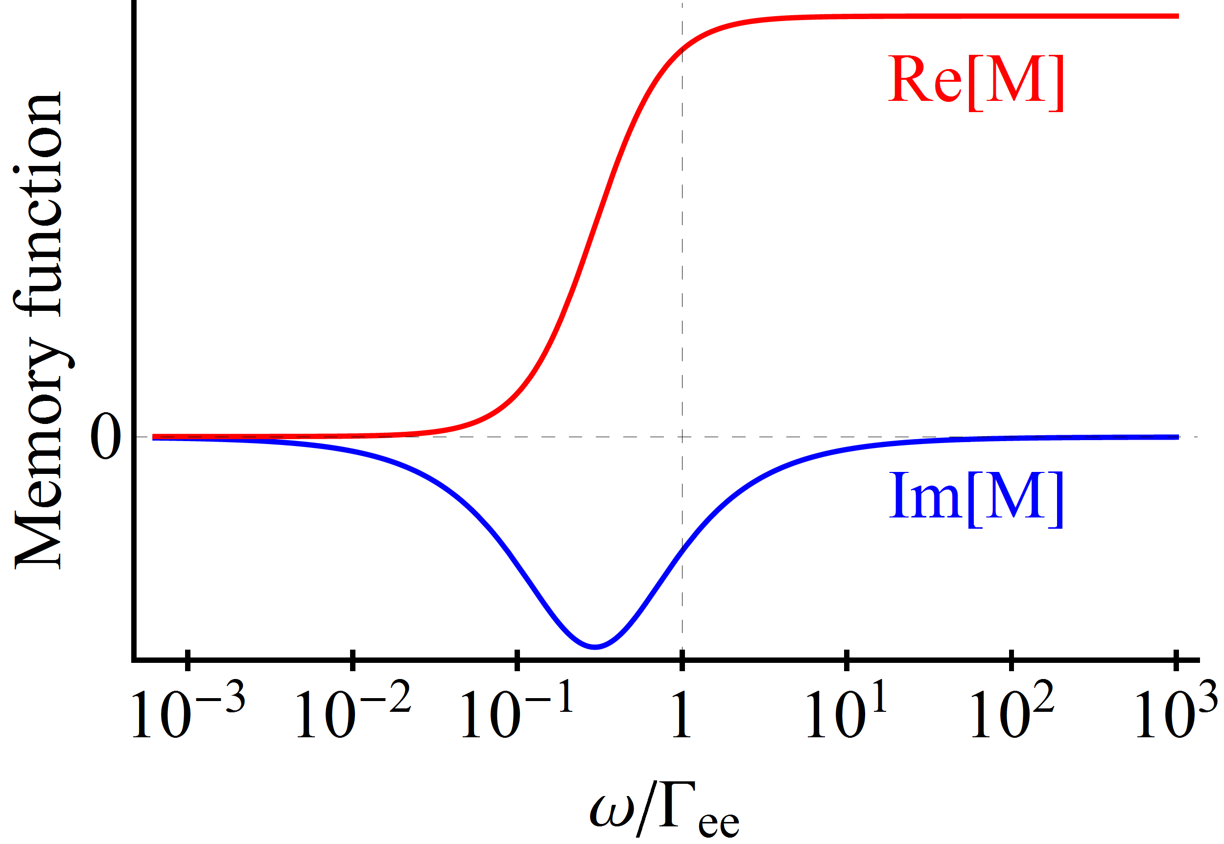
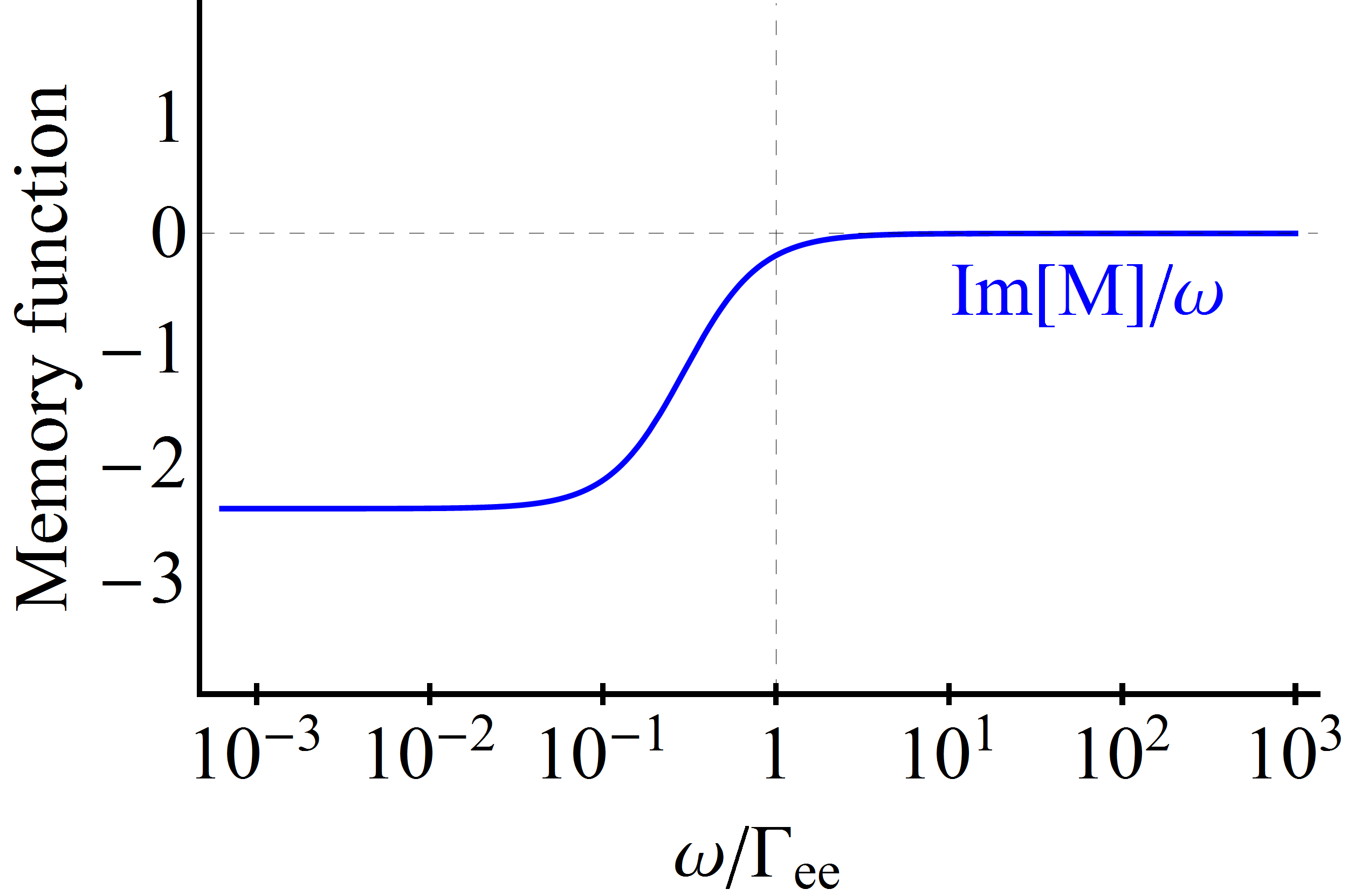
σ⁡(ω)=1π​Dk−i​ω+M⁡(ω),M⁡(ω)≡1τ⁡(ω)−i​ω​λ​(ω).\displaystyle\sigma(\omega)=\frac{1}{\pi}\frac{D_{k}}{-i\omega+M(\omega)}\,,\quad M(\omega)\equiv\frac{1}{\tau(\omega)}-i\omega\lambda(\omega)\,. (S18)

The complex memory function M⁡(ω)M(\omega) appearing in this equation is illustrated by Fig. S1. Both the effective scattering rate 1/τ=Re⁡M⁡(ω)1/\tau=\re M(\omega) and the mass renormalization factor λ=−ImM(ω)/ω\lambda=-\im M(\omega)/\omega show step-like crossovers at the boundary ω∼Γe​e\omega\sim\Gamma_{ee} of the hydrodynamic and kinetic regimes.

Refer to caption
Refer to caption
Figure S1: (Top) Real and imaginary parts of the memory function M⁡(ω)M(\omega) in Eq. (S18). (Bottom) Mass renormalization factor Im⁡M⁡(ω)/ω≡−λ\im M(\omega)/\omega\equiv-\lambda. The wide dynamic range of ω\omega is used to illustrate the features more clearly.

II Second-order conductivity: general

The second-order nonlinear conductivity σi​l​m(2)\sigma_{ilm}^{(2)} determines the second-order current

ji(2)​(𝐪,ω)=∫d​ω′​d2​q′(2​π)3​σi​l​m(2)​(𝐪−𝐪′,ω−ω′,𝐪′,ω′)×El​(𝐪−𝐪′,ω−ω′)​Em​(𝐪′,ω′)\begin{split}j_{i}^{(2)}\left(\mathbf{q},\omega\right)&=\int\frac{d\omega^{\prime}d^{2}{q}^{\prime}}{(2\pi)^{3}}\sigma_{ilm}^{(2)}\left(\mathbf{q}-\mathbf{q}^{\prime},\omega-\omega^{\prime};\mathbf{q}^{\prime},\omega^{\prime}\right)\\ &\times E_{l}\left(\mathbf{q}-\mathbf{q}^{\prime},\omega-\omega^{\prime})E_{m}(\mathbf{q}^{\prime},\omega^{\prime}\right)\end{split} (S19)

in response to the total electric field 𝐄\mathbf{E} in the system. By convention, σi​l​m(2)​(𝐪𝟏,ω1,𝐪𝟐,ω2)\sigma_{ilm}^{(2)}\left(\mathbf{q_{1}},\omega_{1};\mathbf{q_{2}},\omega_{2}\right) is chosen to be symmetrized, i.e., invariant under the interchange (1↔2,l↔m)(1\leftrightarrow 2,l\leftrightarrow m). Expanded to the linear order in momenta, the second-order conductivity must have the form

σi​l​m(2)=Σi​l​m​n​(ω1,ω2)​q1​n+(1↔2l↔m),\displaystyle\sigma^{(2)}_{ilm}=\Sigma_{ilmn}(\omega_{1},\omega_{2})q_{1n}+\left(\begin{smallmatrix}1&\leftrightarrow&2\\ l&\leftrightarrow&m\end{smallmatrix}\right)\,, (S20)

where Σi​l​m​n\Sigma_{ilmn} is some isotropic rank-44 tensor. Any such tensor is a linear combination of the following three:

Bi​l​m​n1=δi​l​δn​m,Bi​l​m​n2=δi​m​δn​l,Bi​l​m​n3=δi​n​δl​m.\displaystyle B^{1}_{ilmn}=\delta_{il}\delta_{nm}\,,\>\>\>B^{2}_{ilmn}=\delta_{im}\delta_{nl}\,,\>\>\>B^{3}_{ilmn}=\delta_{in}\delta_{lm}\,. (S21)

In other words, σi​l​m(2)\sigma^{(2)}_{ilm} is fully characterized by three functions G1G_{1}, G2G_{2}, and G3G_{3} such that

Σi​l​m​n​(ω1,ω2)=∑a=13Ga​(ω1,ω2)​Bi​l​m​na.\displaystyle\Sigma_{ilmn}(\omega_{1},\omega_{2})=\sum_{a=1}^{3}G_{a}(\omega_{1},\omega_{2})B^{a}_{ilmn}\,. (S22)

Below we derive σi​l​m(2)\sigma^{(2)}_{ilm} and show it has a different form in the hydrodynamic and the kinetic regimes.

III Second-order conductivity in the hydrodynamic regime

To derive σi​l​m(2)\sigma_{ilm}^{(2)} in the hydrodynamic regime we solve the equations

∂tn+∂iji=0,ji=n​ui,\displaystyle\partial_{t}n+\partial_{i}j_{i}=0\,,\>\>\>j_{i}=nu_{i}\,, (S23a)
(∂t+ΓE)nE+∂i(γ2Wui)=jmEm,nE=γ2W−P,\displaystyle\left(\partial_{t}+\Gamma_{E}\right)n_{E}+\partial_{i}\left(\gamma^{2}Wu_{i}\right)=j_{m}E_{m}\,,\>\>\>n_{E}=\gamma^{2}W-P\,, (S23b)
(∂t+Γd+uk∂k)ui=1γ2​W(−∂iP−ui∂tP+nEiOPEN+nc​ϵi​k​l​uk​Bl−ui​jm​Em).\displaystyle\begin{aligned} \left(\partial_{t}+\Gamma_{d}+u_{k}\partial_{k}\right)u_{i}&=\frac{1}{\gamma^{2}W}\Biggl(-\partial_{i}P-u_{i}\partial_{t}P+nE_{i}\\ \mbox{}&+\frac{n}{c}\,\epsilon_{ikl}u_{k}B_{l}-u_{i}j_{m}E_{m}\Biggr)\,.\end{aligned} (S23c)

These equations are the same as Eqs. (7) of the main text, except we added phenomenological energy dissipation rate ΓE\Gamma_{E} in Eq. (S23b) and chose the units e=v=1e=v=1 to lighten the notations. Hence, the Lorentz factor in Eq. (S23c) is now γ=1/1−u2\gamma=1/\sqrt{1-u^{2}}. The derivation of Eqs. (S23) can be found in literature [36, 3, 4, 38, 5]. The definitions of pressure PP, energy density nEn_{E}, and enthalpy density WW deserve a comment. Whereas the current 𝐣\mathbf{j} is proportional to the actual charge density nn, the pressure P=P⁡(n0,nE​0)P=P(n_{0},n_{E0}) is the equilibrium thermodynamic parameter, which is a function of the proper density n0=n/γn_{0}=n/\gamma and the proper energy density nE​0n_{E0}. The actual energy density is nEn_{E} [Eq. (S23b)] and the enthalpy density is W=nE​0+PW=n_{E0}+P. Another key thermodynamic parameter is the dimensionless isentropic (ise) bulk modulus CiseC_{\mathrm{ise}}. It is defined by Eq. (10) of the main text:

Cise=n0W​(∂P∂n0)sn=n0W​(∂P∂n0)nE​0+(∂P∂nE​0)n0.\displaystyle\begin{split}C_{\mathrm{ise}}=\frac{n_{0}}{W}\left(\frac{\partial P}{\partial n_{0}}\right)_{s_{n}}=\frac{n_{0}}{W}\left(\frac{\partial P}{\partial n_{0}}\right)_{n_{E0}}+\left(\frac{\partial P}{\partial n_{E0}}\right)_{n_{0}}.\end{split} (S24)

The second equation in Eq. (S24) follows from the thermodynamic relation

T​d​sn=n0−1​d​nE​0−n0−2​W​d​n0Tds_{n}=n_{0}^{-1}dn_{E0}-n_{0}^{-2}Wdn_{0}

for the quantity sn=s/n0s_{n}=s/n_{0}, with s=s⁡(n0,nE​0)s=s(n_{0},n_{E0}) being the entropy density.

Suppose 𝐄⁡(𝐫,t)∝ei​𝐪𝐫−i​ω​t\mathbf{E}(\mathbf{r},t)\propto e^{i\mathbf{q}\mathbf{r}-i\omega t} and define ω+=ω+i​Γd\omega^{+}=\omega+i\Gamma_{d}. To the first order in 𝐄\mathbf{E} we obtain, for ΓE=0\Gamma_{E}=0:

n(1)=n0(1)=n0ωqmu(1)m,nE(1)=nE​0(1)=Wωqmu(1)m,Em(1)=−iω+Wn0u(1)m,W(1)=∂W∂n0​n0(1)+∂W∂nE​0​nE​0(1)=(n0W​∂W∂n0+∂W∂nE​0)​Wω​qm​um=(1+Cise)​Wω​qm​um,P(1)=∂P∂n0​n0(1)+∂P∂nE​0​nE​0(1)=(n0W​∂P∂n0+∂P∂nE​0)​Wω​qm​um=Cise​Wω​qm​um,(nW)(1)=n(1)W−n0​W(1)W2=−Cise​n0W​1ω​qm​um.\begin{split}n^{(1)}&=n_{0}^{(1)}=\frac{n_{0}}{\omega}q_{m}u^{(1)}_{m}\,,\quad n_{E}^{(1)}=n_{E0}^{(1)}=\frac{W}{\omega}q_{m}u^{(1)}_{m}\,,\quad E_{m}^{(1)}=-i\omega^{+}\frac{W}{n_{0}}u^{(1)}_{m}\,,\\ W^{(1)}&=\frac{\partial W}{\partial{n_{0}}}n_{0}^{(1)}+\frac{\partial W}{\partial{n_{E0}}}n_{E0}^{(1)}=\left(\frac{n_{0}}{W}\frac{\partial W}{\partial{n_{0}}}+\frac{\partial W}{\partial{n_{E0}}}\right)\frac{W}{\omega}q_{m}u_{m}=\left(1+C_{\mathrm{ise}}\right)\frac{W}{\omega}q_{m}u_{m}\,,\\ P^{(1)}&=\frac{\partial P}{\partial{n_{0}}}n_{0}^{(1)}+\frac{\partial P}{\partial{n_{E0}}}n_{E0}^{(1)}=\left(\frac{n_{0}}{W}\frac{\partial P}{\partial{n_{0}}}+\frac{\partial P}{\partial{n_{E0}}}\right)\frac{W}{\omega}q_{m}u_{m}=C_{\mathrm{ise}}\frac{W}{\omega}q_{m}u_{m}\,,\\ \left(\frac{n}{W}\right)^{(1)}&=\frac{n^{(1)}}{W}-n_{0}\frac{W^{(1)}}{W^{2}}=-C_{\mathrm{ise}}\frac{n_{0}}{W}\frac{1}{\omega}q_{m}u_{m}\,.\end{split} (S25)

Now let us assume that the electric field consists of two plane waves:

𝐄⁡(𝐫,t)=𝐄1​ei​𝐪1​𝐫−i​ω1​t+𝐄2​ei​𝐪2​𝐫−i​ω2​t+c.c.\mathbf{E}(\mathbf{r},t)=\mathbf{E}_{1}e^{i\mathbf{q}_{1}\mathbf{r}-i\omega_{1}t}+\mathbf{E}_{2}e^{i\mathbf{q}_{2}\mathbf{r}-i\omega_{2}t}+\mathrm{c.c.} (S26)

To the second order in 𝐄\mathbf{E}, various quantities of interest develop Fourier amplitudes of frequency and momenta (𝐪3,ω3)=(𝐪1+𝐪2,ω1+ω2)(\mathbf{q}_{3},\,\omega_{3})=(\mathbf{q}_{1}+\mathbf{q}_{2},\,\omega_{1}+\omega_{2}). These amplitudes are given by

n(2)=O(qν2u),n0(2)=n(2)−12n0u2=−12n0u(1)1​iu(1)2​i+(1↔2)+O(qν2),nE(2)=ω2+ω3Wu(1)1​iu(1)2​i+(1↔2)+O(qν2),nE​0(2)=n(2)E−Wu2=i​Γd−ω1ω3Wu(1)1​iu(1)2​i+(1↔2)+O(qν2),P(2)=n0(2)​∂P∂n0+nE​0(2)​∂P∂nE​0+12​{[n0(1)]2​∂2P∂n02+2​n0(1)​nE​0(1)​∂2P∂n0​∂nE​0+[nE​0(1)]2​∂2P∂nE​02}=−12​n0​u1​i(1)​u2​i(1)​∂P∂n0+i​Γd−ω1ω3​u1​i(1)​u2​i(1)​W​∂P∂nE​0+(1↔2)+O⁡(qν2)=(−Cise+2​i​Γdω3​∂P∂nE​0)​W​u1​i(1)​u2​i(1)+O⁡(qν2).\begin{split}n^{(2)}&=O\left(q_{\nu}^{2}u\right)\,,\quad n_{0}^{(2)}=n^{(2)}-\frac{1}{2}n_{0}u^{2}=-\frac{1}{2}n_{0}u^{(1)}_{1i}u^{(1)}_{2i}+(1\leftrightarrow 2)+O\left(q_{\nu}^{2}\right)\,,\\ n_{E}^{(2)}&=\frac{\omega_{2}^{+}}{\omega_{3}}Wu^{(1)}_{1i}u^{(1)}_{2i}+(1\leftrightarrow 2)+O\left(q_{\nu}^{2}\right)\,,\quad n_{E0}^{(2)}=n^{(2)}_{E}-Wu^{2}=\frac{i\Gamma_{d}-\omega_{1}}{\omega_{3}}Wu^{(1)}_{1i}u^{(1)}_{2i}+(1\leftrightarrow 2)+O\left(q_{\nu}^{2}\right)\,,\\ P^{(2)}&=n^{(2)}_{0}\frac{\partial P}{\partial n_{0}}+n^{(2)}_{E0}\frac{\partial P}{\partial n_{E0}}+\frac{1}{2}\left\{\left[{n_{0}^{(1)}}\right]^{2}\frac{\partial^{2}P}{\partial{n_{0}}^{2}}+2n_{0}^{(1)}n_{E0}^{(1)}\frac{\partial^{2}P}{\partial{n_{0}}\partial{n_{E0}}}+\left[{n_{E0}^{(1)}}\right]^{2}\frac{\partial^{2}P}{\partial{n_{E0}}^{2}}\right\}\\ &=-\frac{1}{2}n_{0}u^{(1)}_{1i}u^{(1)}_{2i}\frac{\partial P}{\partial n_{0}}+\frac{i\Gamma_{d}-\omega_{1}}{\omega_{3}}u^{(1)}_{1i}u^{(1)}_{2i}W\frac{\partial P}{\partial n_{E0}}+(1\leftrightarrow 2)+O\left(q_{\nu}^{2}\right)=\left(-C_{\mathrm{ise}}+\frac{2i\Gamma_{d}}{\omega_{3}}\frac{\partial P}{\partial n_{E0}}\right)Wu^{(1)}_{1i}u^{(1)}_{2i}+O\left(q_{\nu}^{2}\right)\,.\end{split} (S27)

From Eq. (S23c) and the Faraday law ϵi​k​l∂kEl=−c−1∂tBi\epsilon_{ikl}\partial_{k}E_{l}=-c^{-1}\partial_{t}B_{i} we obtain

(∂t+Γd+uk∂k)ui\displaystyle(\partial_{t}+\Gamma_{d}+u_{k}\partial_{k})u_{i} =nγ2​WA^i​j(−i∂,i∂t)Ej−1γ2​W(∂iP+ui∂tP)−1γ2​WuijmEm,\displaystyle=\frac{n}{\gamma^{2}W}\hat{A}_{ij}\left(-i\bm{\partial},\,i\partial_{t}\right)E_{j}-\frac{1}{\gamma^{2}W}(\partial_{i}P+u_{i}\partial_{t}P)-\frac{1}{\gamma^{2}W}u_{i}j_{m}E_{m}\,, (S28)
A^i​j​(𝐤,ω)\displaystyle\hat{A}_{ij}\left(\mathbf{k},\omega\right) =(1−km​umω)​δi​j+ki​ujω.\displaystyle=\left(1-\frac{k_{m}u_{m}}{\omega}\right)\delta_{ij}+\frac{k_{i}u_{j}}{\omega}\,. (S29)

Keeping only the terms linear in 𝐪ν\mathbf{q}_{\nu}, we find

−i​ω3+​ui(2)=−i​q2​k​u1​k(1)​u2​i(1)+n0W​(−q2​mω2​u1​m(1)​E2​i+q2​iω2​u1​m(1)​E2​m)+(nW)1(1)​E2​i(1)−1W​(i2​q3​i​P(2)−i​ω1​P1(1)​u2​i(1))+(1↔2)=−i​q2​i​u1​m(1)​u2​m(1)−Γdω2​q2​m​u1​m(1)​u2​i(1)+Γdω2​q2​i​u1​m(1)​u2​m(1)+i​Cise​ω2+ω1​q1​m​u1​m(1)​u2​i(1)+i​Cise​q2​m​u1​i(1)​u2​m(1)+i2​Cise​q3​i​u1​m(1)​u2​m(1)+∂P∂nE​0​Γdω3​q3​i​u1​m(1)​u2​m(1)+(1↔2).\begin{split}-i\omega_{3}^{+}u_{i}^{(2)}&=-i{q_{2k}}u_{1k}^{(1)}u^{(1)}_{2i}+\frac{n_{0}}{W}\left(-\frac{q_{2m}}{\omega_{2}}u_{1m}^{(1)}E_{2i}+\frac{q_{2i}}{\omega_{2}}u_{1m}^{(1)}E_{2m}\right)+\left(\frac{n}{W}\right)_{1}^{(1)}E_{2i}^{(1)}-\frac{1}{W}\left(\frac{i}{2}q_{3i}P^{(2)}-i\omega_{1}P_{1}^{(1)}u_{2i}^{(1)}\right)+(1\leftrightarrow 2)\\ &=-iq_{2i}u_{1m}^{(1)}u^{(1)}_{2m}-\frac{\Gamma_{d}}{\omega_{2}}q_{2m}u_{1m}^{(1)}u^{(1)}_{2i}+\frac{\Gamma_{d}}{\omega_{2}}q_{2i}u_{1m}^{(1)}u^{(1)}_{2m}\\ &\mbox{}+iC_{\mathrm{ise}}\frac{\omega_{2}^{+}}{\omega_{1}}q_{1m}u_{1m}^{(1)}u^{(1)}_{2i}+iC_{\mathrm{ise}}q_{2m}u_{1i}^{(1)}u^{(1)}_{2m}+\frac{i}{2}C_{\mathrm{ise}}q_{3i}u_{1m}^{(1)}u^{(1)}_{2m}+\frac{\partial P}{\partial n_{E0}}\frac{\Gamma_{d}}{\omega_{3}}q_{3i}u_{1m}^{(1)}u^{(1)}_{2m}+(1\leftrightarrow 2)\,.\end{split} (S30)

The current to the second order in field is

ji(2)\displaystyle j_{i}^{(2)} =n(1)​ui(1)+n(0)​ui(2)\displaystyle=n^{(1)}u^{(1)}_{i}+n^{(0)}u^{(2)}_{i} (S31)
=n0ω3+​(ω3+ω1​q1​m​u1​m(1)​u2​i(1)+q2​i​u1​m(1)​u2​m(1)−i​Γdω2​q2​m​u1​m(1)​u2​i(1)+i​Γdω2​q2​i​u1​m(1)​u2​m(1)CLOSE\displaystyle=\frac{n_{0}}{\omega_{3}^{+}}\bigg(\frac{\omega_{3}^{+}}{\omega_{1}}q_{1m}u^{(1)}_{1m}u^{(1)}_{2i}+q_{2i}u_{1m}^{(1)}u^{(1)}_{2m}-\frac{i\Gamma_{d}}{\omega_{2}}q_{2m}u_{1m}^{(1)}u^{(1)}_{2i}+\frac{i\Gamma_{d}}{\omega_{2}}q_{2i}u_{1m}^{(1)}u^{(1)}_{2m}
OPEN−Cise​ω2+ω1​q1​m​u1​m(1)​u2​i(1)−Cise​q2​m​u1​i(1)​u2​m(1)−12​Cise​q3​i​u1​m(1)​u2​m(1)+∂P∂nE​0​i​Γdω3​q3​i​u1​m(1)​u2​m(1))+(1↔2)\displaystyle-C_{\mathrm{ise}}\frac{\omega_{2}^{+}}{\omega_{1}}q_{1m}u_{1m}^{(1)}u^{(1)}_{2i}-C_{\mathrm{ise}}q_{2m}u_{1i}^{(1)}u^{(1)}_{2m}-\frac{1}{2}C_{\mathrm{ise}}q_{3i}u_{1m}^{(1)}u^{(1)}_{2m}+\frac{\partial P}{\partial n_{E0}}\frac{i\Gamma_{d}}{\omega_{3}}q_{3i}u_{1m}^{(1)}u^{(1)}_{2m}\bigg)+(1\leftrightarrow 2)
=n0ω3+​(ω3+ω1​q1​β​δi​ν+ω3+ω2​q2​ν​δi​β+q3​i​δβ​ν−Cise​ω2+ω1​q1​β​δi​ν−Cise​ω1+ω2​q2​ν​δi​β−Cise​q2​ν​δi​β−Cise​q1​β​δi​ν−Cise​q3​i​δν​βCLOSE\displaystyle=\frac{n_{0}}{\omega_{3}^{+}}\bigg(\frac{\omega_{3}^{+}}{\omega_{1}}q_{1\beta}\delta_{i\nu}+\frac{\omega_{3}^{+}}{\omega_{2}}q_{2\nu}\delta_{i\beta}+q_{3i}\delta_{\beta\nu}-C_{\mathrm{ise}}\frac{\omega_{2}^{+}}{\omega_{1}}q_{1\beta}\delta_{i\nu}-C_{\mathrm{ise}}\frac{\omega_{1}^{+}}{\omega_{2}}q_{2\nu}\delta_{i\beta}-C_{\mathrm{ise}}q_{2\nu}\delta_{i\beta}-C_{\mathrm{ise}}q_{1\beta}\delta_{i\nu}-C_{\mathrm{ise}}q_{3i}\delta_{\nu\beta}
OPEN−i​Γdω2​q2​β​δi​ν−i​Γdω1​q1​ν​δi​β+i​Γdω2​q2​i​δβ​ν+i​Γdω1​q1​i​δβ​ν+∂P∂nE​0​2​i​Γdω3​q3​i​δν​β)​u1​β(1)​u2​ν(1)\displaystyle-\frac{i\Gamma_{d}}{\omega_{2}}q_{2\beta}\delta_{i\nu}-\frac{i\Gamma_{d}}{\omega_{1}}q_{1\nu}\delta_{i\beta}+\frac{i\Gamma_{d}}{\omega_{2}}q_{2i}\delta_{\beta\nu}+\frac{i\Gamma_{d}}{\omega_{1}}q_{1i}\delta_{\beta\nu}+\frac{\partial P}{\partial n_{E0}}\frac{2i\Gamma_{d}}{\omega_{3}}q_{3i}\delta_{\nu\beta}\bigg)u_{1\beta}^{(1)}u^{(1)}_{2\nu}
=n0ω3+[(1−Cise)(ω3+ω1q1​βδi​ν+ω3+ω2q2​νδi​β+q3​iδβ​ν)\displaystyle=\frac{n_{0}}{\omega_{3}^{+}}\Bigg[(1-C_{\mathrm{ise}})\left(\frac{\omega_{3}^{+}}{\omega_{1}}q_{1\beta}\delta_{i\nu}+\frac{\omega_{3}^{+}}{\omega_{2}}q_{2\nu}\delta_{i\beta}+q_{3i}\delta_{\beta\nu}\right)
+iΓd(−q2​βω2δi​ν−q1​νω1δi​β+q2​iω2δβ​ν+q1​iω1δβ​ν+∂P∂nE​02​q3​iω3δν​β)]u1​β(1)u2​ν(1).\displaystyle+{i\Gamma_{d}}\left(-\frac{q_{2\beta}}{\omega_{2}}\delta_{i\nu}-\frac{q_{1\nu}}{\omega_{1}}\delta_{i\beta}+\frac{q_{2i}}{\omega_{2}}\delta_{\beta\nu}+\frac{q_{1i}}{\omega_{1}}\delta_{\beta\nu}+\frac{\partial P}{\partial n_{E0}}\frac{2q_{3i}}{\omega_{3}}\delta_{\nu\beta}\right)\Bigg]u_{1\beta}^{(1)}u^{(1)}_{2\nu}\,. (S32)

Hence, the second-order conductivity is

σi​l​m(2)\displaystyle\sigma^{(2)}_{ilm} =Dh(2)ω1+​ω2+​ω3+​{ω3+ω1​q1​l​δi​m+q1​i​δl​m+i​Γd1−Cise​[(q1​iω1+∂P∂nE​2​q1​iω3+i​ΓE)​δl​m−q1​mω1​δi​l]}+(1↔2l↔m).\displaystyle=\frac{D^{(2)}_{h}}{\omega_{1}^{+}\omega_{2}^{+}\omega_{3}^{+}}\left\{\frac{\omega_{3}^{+}}{\omega_{1}}q_{1l}\delta_{im}+q_{1i}\delta_{lm}+\frac{i\Gamma_{d}}{1-C_{\mathrm{ise}}}\left[\left(\frac{q_{1i}}{\omega_{1}}+\frac{\partial P}{\partial n_{E}}\frac{2q_{1i}}{\omega_{3}+i\Gamma_{E}}\right)\delta_{lm}-\frac{q_{1m}}{\omega_{1}}\delta_{il}\right]\right\}+\left(\begin{smallmatrix}1&\leftrightarrow&2\\ l&\leftrightarrow&m\end{smallmatrix}\right)\,. (S33)

Here we added the neglected earlier energy dissipation rate ΓE\Gamma_{E} in one of the terms in Eq. (S33). In principle, ΓE\Gamma_{E} should appear in more than one place. However, we assume that ΓE\Gamma_{E} is very small and its sole role is to resolve the indeterminacy of the ratio q3/ω3q_{3}/\omega_{3} in the context of the photon drag problem where q3,ω3→0q_{3},\omega_{3}\to 0. The second-order spectral weight appearing in Eq. (S33) is

Dh(2)=−e3​n3​v42​W2​(1−Cise)=−12​e3​nm∗2​(1−Cise),D^{(2)}_{h}=-\frac{e^{3}n^{3}v^{4}}{2W^{2}}(1-C_{\mathrm{ise}})=-\frac{1}{2}\frac{e^{3}n}{m^{\ast 2}}(1-C_{\mathrm{ise}})\,, (S34)

where we restored physical units and replaced n0n_{0} by nn, nE​0n_{E0} by nEn_{E} to simplify notations. Let us discuss the value of Dh(2)D^{(2)}_{h} in representative cases, assuming ee interaction corrections to pressure and enthalpy density are negligible. The result for particles with a parabolic dispersion can be obtained taking the nonrelativistic limit, in which P≃(2/d)​(nE−n​m​v2)P\simeq({2}/{d})(n_{E}-nmv^{2}) and W≃n​m​v2W\simeq nmv^{2}. This gives

Dh(2)=−12​e3​nm2,∂P∂nE=2d,Cise≪1.\displaystyle D^{(2)}_{h}=-\frac{1}{2}\frac{e^{3}n}{m^{2}}\,,\quad\frac{\partial P}{\partial n_{E}}=\frac{2}{d}\,,\quad C_{\mathrm{ise}}\ll 1\,. (S35)

In the massless case, one finds P=nE/dP=n_{E}/d and W=(1+1/d)​nEW=(1+1/d)n_{E}, so that

Dh(2)=−d⁡(d−1)2​(d+1)2​e3​n3​v4nE2,∂P∂nE=1d,Cise=1d.\displaystyle D^{(2)}_{h}=-\frac{d(d-1)}{2(d+1)^{2}}\frac{e^{3}n^{3}v^{4}}{n_{E}^{2}}\,,\quad\frac{\partial P}{\partial n_{E}}=\frac{1}{d}\,,\quad C_{\mathrm{ise}}=\frac{1}{d}\,. (S36)

Taking d=2d=2 for graphene, we get

Dh(2)\displaystyle D^{(2)}_{h} =−e3​n3​v49​nE2,\displaystyle=-\frac{e^{3}n^{3}v^{4}}{9n_{E}^{2}}\,, (S37)
Dh(2)​(T=0)\displaystyle D^{(2)}_{h}(T=0) =−g16​π​e3​v2ℏ2≡2​D0(2).\displaystyle=-\frac{g}{16\pi}\frac{e^{3}v^{2}}{\hbar^{2}}\equiv 2D^{(2)}_{0}\,. (S38)

Functions G1G_{1}, G2G_{2}, and G3G_{3} [Eq. (S22)] corresponding to Eq. (S33) are

G1=Dh(2)ω1+​ω2+​ω3+​(−11−Cise​i​Γdω1),G2=Dh(2)ω1+​ω2+​ω3+​(ω3+ω1),G3=Dh(2)ω1+​ω2+​ω3+​[1+i​Γd1−Cise​(1ω1+∂P∂nE​2ω3+i​ΓE)].\begin{split}G_{1}&=\frac{D^{(2)}_{h}}{\omega_{1}^{+}\omega_{2}^{+}\omega_{3}^{+}}\left(-\frac{1}{1-C_{\mathrm{ise}}}\frac{i\Gamma_{d}}{\omega_{1}}\right)\,,\\ G_{2}&=\frac{D^{(2)}_{h}}{\omega_{1}^{+}\omega_{2}^{+}\omega_{3}^{+}}\left(\frac{\omega_{3}^{+}}{\omega_{1}}\right)\,,\\ G_{3}&=\frac{D^{(2)}_{h}}{\omega_{1}^{+}\omega_{2}^{+}\omega_{3}^{+}}\left[1+\frac{i\Gamma_{d}}{1-C_{\mathrm{ise}}}\left(\frac{1}{\omega_{1}}+\frac{\partial P}{\partial{n_{E}}}\frac{2}{\omega_{3}+i\Gamma_{E}}\right)\right]\,.\end{split} (S39)

In the collisionless limit Γd→0\Gamma_{d}\to 0, these formulas simplify to

(G1,G2,G3)=Dh(2)​(0,1ω12​ω2,1ω1​ω2​ω3),\displaystyle(G_{1},G_{2},G_{3})=D^{(2)}_{h}\left(0,\,\frac{1}{\omega_{1}^{2}\omega_{2}},\,\frac{1}{\omega_{1}\omega_{2}\omega_{3}}\right)\,, (S40)

while Eq. (S33) reduces to

σi​l​m(2)=Dh(2)ω1​ω2​ω3​(ω3ω1​q1​l​δi​m+ω3ω2​q2​m​δi​l+q3​i​δl​m),\displaystyle\sigma^{(2)}_{ilm}=\frac{D^{(2)}_{h}}{\omega_{1}\omega_{2}\omega_{3}}\bigg(\frac{\omega_{3}}{\omega_{1}}q_{1l}\delta_{im}+\frac{\omega_{3}}{\omega_{2}}q_{2m}\delta_{il}+q_{3i}\delta_{lm}\bigg)\,, (S41)

which is equivalent to Eq. (2) of the main text.

IV Second-order conductivity in the kinetic regime

The kinetic regime corresponds to the frequency range Γe​e≪ω≪εF\Gamma_{ee}\ll\omega\ll\varepsilon_{F}. The linear and nonlinear conductivities in this regime can be computed by solving the Boltzmann kinetic equation

[∂t+𝐯⋅∂+(𝐄+𝐯c×𝐁)∂𝐩]f=I^[f].\displaystyle\left[\partial_{t}+\mathbf{v}\cdot\bm{\partial}+\left(\mathbf{E}+\frac{\mathbf{v}}{c}\times\mathbf{B}\right)\bm{\partial}_{\mathbf{p}}\right]f=\hat{I}\left[f\right]\,. (S42)

In this section, we again set e=1e=1 and suppress the subscripts 𝐩{\mathbf{p}} in 𝐯𝐩\mathbf{v}_{\mathbf{p}}, f𝐩f_{\mathbf{p}}. One should not confuse the quasiparticle velocity 𝐯\mathbf{v} at finite 𝐩\mathbf{p}, a vector, with vv, the limiting velocity at p=∞p=\infty, a scalar.

The magnetic-field term in Eq. (S42) can be expressed with the help of the kernel

Ai​j​(𝐤,ω)=(1−km​vmω)​δi​j+ki​vjω,{A}_{ij}\left(\mathbf{k},\omega\right)=\left(1-\frac{k_{m}v_{m}}{\omega}\right)\delta_{ij}+\frac{k_{i}v_{j}}{\omega}\,, (S43)

similar to Eq. (S29), leading to

[∂t+vi∂i+Ai​j(−i∂,i∂t)Ej∂pi]f=I^[f].\left[\partial_{t}+v_{i}\partial_{i}+{A}_{ij}\left(-i\bm{\partial},i\partial_{t}\right)E_{j}\partial_{p_{i}}\right]f=\hat{I}\left[f\right]\,. (S44)

The second-order current we want to compute is

ji​(𝐪3,ω3)=∑vi​f(2)​(𝐪3,ω3).\displaystyle j_{i}\left(\mathbf{q}_{3},\omega_{3}\right)=\sum v_{i}f^{(2)}\left(\mathbf{q}_{3},\omega_{3}\right)\,. (S45)

To do this we need to specify the collision integral I^​[f]\hat{I}\left[f\right].

IV.1 Nonconserving relaxation-time approximation

It is useful to consider first the approximation I^​[f]=−Γ⁡(f−f(0))\hat{I}\left[f\right]=-\Gamma\left(f-f^{(0)}\right), with Γ\Gamma being an energy-independent relaxation rate. This is probably the simplest model one can study. However, one should keep in mind that this approximation is flawed because it may not conserve the particle number.

Assuming the electric field is composed of two plane waves [Eq. (S26)], we expand ff to the first and second order in field:

f(1)​(𝐪ν,ων)\displaystyle f^{(1)}\left(\mathbf{q}_{\nu},\omega_{\nu}\right) =−i​E2​m​vmων+−vk​qν​k∂εf(0),ν=1,2,\displaystyle=\frac{-iE_{2m}v_{m}}{\omega_{\nu}^{+}-v_{k}q_{\nu\,k}}\partial_{\varepsilon}f^{(0)}\,,\quad\nu=1,2\,, (S46)
f(2)​(𝐪3,ω3)\displaystyle f^{(2)}\left(\mathbf{q}_{3},\omega_{3}\right) =−i​E1​l​Aa​l​(𝐪1,ω1)ω3+−vj​q3​j​∂paf(1)​(𝐪2,ω2)+(1↔2).\displaystyle=\frac{-iE_{1l}A_{al}\left(\mathbf{q}_{1},\omega_{1}\right)}{\omega_{3}^{+}-v_{j}q_{3j}}\partial_{p_{a}}f^{(1)}\left(\mathbf{q}_{2},\omega_{2}\right)+(1\leftrightarrow 2)\,. (S47)

Hence, the second-order conductivity is

σi​l​m(2)=−∑Aa​l(𝐪1,ω1)viω3+−vj​q3​j∂pavmω2+−vk​q2​k∂εf(0)+(1↔2l↔m).\displaystyle\sigma^{(2)}_{ilm}=-\sum A_{al}\left(\mathbf{q}_{1},\omega_{1}\right)\frac{v_{i}}{\omega_{3}^{+}-v_{j}q_{3j}}\partial_{p_{a}}\frac{v_{m}}{\omega_{2}^{+}-v_{k}q_{2k}}\partial_{\varepsilon}f^{(0)}+\left(\begin{smallmatrix}1&\leftrightarrow&2\\ l&\leftrightarrow&m\end{smallmatrix}\right)\,. (S48)

The evaluation of this expression for Dirac electrons in graphene is tedious but straightforward. The final result is

σi​l​m(2)\displaystyle\sigma^{(2)}_{ilm} =Dk(2)ω1+​ω2+​ω3+[(ω3ω3+q3−ω1+2​ω2+q2−ω2+2​ω1+q1+2​i​Γω1q1+2​i​Γω2q2)iδl​m\displaystyle=\frac{D_{k}^{(2)}}{\omega_{1}^{+}\omega_{2}^{+}\omega_{3}^{+}}\Bigg[\left(\frac{\omega_{3}}{\omega_{3}^{+}}q_{3}-\frac{\omega_{1}^{+}}{2\omega_{2}^{+}}q_{2}-\frac{\omega_{2}^{+}}{2\omega_{1}^{+}}q_{1}+\frac{2i\Gamma}{\omega_{1}}q_{1}+\frac{2i\Gamma}{\omega_{2}}q_{2}\right)_{i}\delta_{lm}
+(2q2−2q1−ω2+ω1+q1+3​ω1+ω2+q2+2​i​Γω3+q3−4​i​Γω1q1)mδi​l]+(1↔2l↔m).\displaystyle+\left(2q_{2}-2q_{1}-\frac{\omega_{2}^{+}}{\omega_{1}^{+}}q_{1}+\frac{3\omega_{1}^{+}}{\omega_{2}^{+}}q_{2}+\frac{2i\Gamma}{\omega_{3}^{+}}q_{3}-\frac{4i\Gamma}{\omega_{1}}q_{1}\right)_{m}\delta_{il}\Bigg]+\left(\begin{smallmatrix}1&\leftrightarrow&2\\ l&\leftrightarrow&m\end{smallmatrix}\right)\,. (S49)

Its collisionless limit Γ→0\Gamma\to 0 is

σi​l​m(2)\displaystyle\sigma^{(2)}_{ilm} =Dk(2)ω1​ω2​ω3​[(q3−ω12​ω2​q2−ω22​ω1​q1)i​δl​m+(2​q2−2​q1−ω2ω1​q1+3​ω1ω2​q2)m​δi​l]+(1↔2l↔m),\displaystyle=\frac{D_{k}^{(2)}}{\omega_{1}\omega_{2}\omega_{3}}\Bigg[\left(q_{3}-\frac{\omega_{1}}{2\omega_{2}}q_{2}-\frac{\omega_{2}}{2\omega_{1}}q_{1}\right)_{i}\delta_{lm}+\left(2q_{2}-2q_{1}-\frac{\omega_{2}}{\omega_{1}}q_{1}+\frac{3\omega_{1}}{\omega_{2}}q_{2}\right)_{m}\delta_{il}\Bigg]+\left(\begin{smallmatrix}1&\leftrightarrow&2\\ l&\leftrightarrow&m\end{smallmatrix}\right)\,, (S50)

which implies [cf. Eq. (S22)]

(G1,G2,G3)=Dk(2)ω1​ω2​ω3​(−2−ω2ω1, 2+3​ω2ω1, 2−ω2ω1).\displaystyle(G_{1},\,G_{2},\,G_{3})=\frac{D^{(2)}_{k}}{\omega_{1}\omega_{2}\omega_{3}}\left(-2-\frac{\omega_{2}}{\omega_{1}},\,2+3\,\frac{\omega_{2}}{\omega_{1}},\,2-\frac{\omega_{2}}{\omega_{1}}\right)\,. (S51)

The second-order spectral weight in these equations is

Dk(2)=D0(2)​(2​fp=0(0)−1)=D0(2)​tanh⁡(μ2​T),D_{k}^{(2)}=D_{0}^{(2)}\left(2f_{p=0}^{(0)}-1\right)=D_{0}^{(2)}\tanh\left(\frac{\mu}{2T}\right)\,, (S52)

where [Eq. (S38)]

D0(2)=−g32​π​e3​v2ℏ2.D^{(2)}_{0}=-\frac{g}{32\pi}\frac{e^{3}v^{2}}{\hbar^{2}}\,. (S53)

In the limit of T→0T\to 0, we have Dk(2)=D0(2)​sign​(μ)D_{k}^{(2)}=D_{0}^{(2)}\,\mathrm{sign}(\mu). At T≫μT\gg\mu, the asymptotic behavior of the chemical potential is μ∝n/T\mu\propto n/T, see, e.g., Supplemental material of Ref. 12. Therefore, Dk(2)∝n/T2D_{k}^{(2)}\propto n/T^{2} as mentioned in the main text. However, at high TT, an interband contribution to σi​l​m(2)\sigma^{(2)}_{ilm}, not included in our semiclassical approach, may become important.

IV.2 Multiple relaxation-time approximation

Let us assume now that the collision operator I^​[f]\hat{I}\left[f\right] is linear and diagonal in the angular momentum basis, so that the Boltzmann equation can be written as

L^f=−EjAi​j∂pif,L^=L^0(ω)+𝐯⋅∂,\displaystyle\hat{L}f=-E_{j}A_{ij}\partial_{p_{i}}f\,,\quad\hat{L}=\hat{L}_{0}(\omega)+\mathbf{v}\cdot\bm{\partial}\,, (S54)

where L^0\hat{L}_{0} is the operator

L^0=∑l=−∞∞(∂t+Γl)|l⟩⟨l|\displaystyle\hat{L}_{0}=\sum\limits_{l=-\infty}^{\infty}(\partial_{t}+\Gamma_{l})|l\rangle\langle l| (S55)

and Γl\Gamma_{l} is the scattering rate for the angular momentum ll. This rate may depend on the quasiparticle energy ε\varepsilon. The model conserves the number of particles if Γ0=0\Gamma_{0}=0. The action of L^0\hat{L}_{0} can be written in terms of the complex frequencies

ων(μ)=ων+iΓμ,ν=1, 2, 3.\omega_{\nu}^{(\mu)}=\omega_{\nu}+i\Gamma_{\mu}\,,\quad\nu=1,\,2,\,3\,. (S56)

Instead of Eq. (S47) we now get a more complicated expression:

f(2)=L^−1​El​Ai​l​∂piL^−1​Ej​Ai​j​∂pif(0).f^{(2)}=\hat{L}^{-1}E_{l}A_{il}\partial_{p_{i}}\hat{L}^{-1}E_{j}A_{ij}\partial_{p_{i}}f^{(0)}\,. (S57)

To calculate σi​l​m(2)​(𝐪1,ω1,𝐪2,ω2)\sigma_{ilm}^{(2)}(\mathbf{q}_{1},\omega_{1};\mathbf{q}_{2},\omega_{2}) we need the (𝐪3,ω3)(\mathbf{q}_{3},\omega_{3}) Fourier harmonic of f(2)f^{(2)}:

f(2)=L^−1(𝐪3,ω3)E1​l(∂pl−q1​nω1vn∂pl+q1​nω1vl∂pn)L^−1(𝐪2,ω2)E2​mvm∂εf(0)+(1↔2l↔m).\displaystyle f^{(2)}=\hat{L}^{-1}{\left(\mathbf{q}_{3},\omega_{3}\right)}E_{1l}\left(\partial_{p_{l}}-\frac{q_{1n}}{\omega_{1}}v_{n}\partial_{p_{l}}+\frac{q_{1n}}{\omega_{1}}v_{l}\partial_{p_{n}}\right)\hat{L}^{-1}{\left(\mathbf{q}_{2},\omega_{2}\right)}E_{2m}v_{m}\partial_{\varepsilon}f^{(0)}+\left(\begin{smallmatrix}1&\leftrightarrow&2\\ l&\leftrightarrow&m\end{smallmatrix}\right)\,. (S58)

[The argument (𝐪3,ω3)(\mathbf{q}_{3},\omega_{3}) of f(2)f^{(2)} is omitted.] For our purpose of computing the terms linear in gradients the expansion

L^−1≃R^−R^(𝐯⋅∂)R^,R^=L^0−1\displaystyle\hat{L}^{-1}\simeq\hat{R}-\hat{R}\left(\mathbf{v}\cdot\bm{\partial}\right)\hat{R}\,,\quad\hat{R}=\hat{L}_{0}^{-1} (S59)

suffices. It yields

f(2)=E1​lE2​m[R^(ω3)(−1ω1q1​nvn∂pl+1ω1vlq1​n∂pn)R^(ω2)−R^(ω3)iq3​iviR^(ω3)∂plR^(ω2)−R^(ω3)∂plR^(ω2)iq2​iviR^(ω2)]vm∂εf(0)+(1↔2l↔m).\begin{split}f^{(2)}&=E_{1l}E_{2m}\Bigg[\hat{R}{(\omega_{3})}\left(-\frac{1}{\omega_{1}}q_{1n}v_{n}\partial_{p_{l}}+\frac{1}{\omega_{1}}v_{l}q_{1n}\partial_{p_{n}}\right)\hat{R}{(\omega_{2})}-\hat{R}{(\omega_{3})}iq_{3i}v_{i}\hat{R}{(\omega_{3})}\partial_{p_{l}}\hat{R}{(\omega_{2})}\\ \mbox{}&-\hat{R}{(\omega_{3})}\partial_{p_{l}}\hat{R}{(\omega_{2})}iq_{2i}v_{i}\hat{R}{(\omega_{2})}\Bigg]v_{m}\partial_{\varepsilon}f^{(0)}+\left(\begin{smallmatrix}1&\leftrightarrow&2\\ l&\leftrightarrow&m\end{smallmatrix}\right)\,.\end{split} (S60)

To do the summation over the angular directions, we expand all the variables in the angular momentum basis. To this end, we do a set of unitary transformations. For example, the velocity goes from 𝐯=(vx,vy)T=|𝐯|​(cos⁡ϕ,sin⁡ϕ)T\mathbf{v}=\left(v_{x},v_{y}\right)^{T}=\left|\mathbf{v}\right|\left(\cos\phi,\,\sin\phi\right)^{T} to (v~−,v~+)T\left(\tilde{v}_{-},\tilde{v}_{+}\right)^{T}:

(v~+v~−)=𝐔(vxvy)=|𝐯|2(M+M−),𝐔={Um​j}=12(1+i1−i),𝐔𝐔†={δi​j},Mm=ei​m​ϕ,m=±.\begin{pmatrix}\tilde{v}_{+}\\ \tilde{v}_{-}\end{pmatrix}=\mathbf{U}\,\begin{pmatrix}v_{x}\\ v_{y}\end{pmatrix}=\frac{\left|\mathbf{v}\right|}{\sqrt{2}}\begin{pmatrix}M_{+}\\ M_{-}\end{pmatrix}\,,\quad\mathbf{U}=\left\{U_{mj}\right\}=\frac{1}{\sqrt{2}}\begin{pmatrix}1&+i\\ 1&-i\end{pmatrix}\,,\quad\mathbf{U}\mathbf{U}^{\dagger}=\{\delta_{ij}\}\,,\quad M_{m}=e^{im\phi}\,,\quad m=\pm\,. (S61)

We do the same transformation for the momentum-space derivatives:

∂~pm=Um​j∂pj=12(∂px+im∂py)=Mm(∂p+imp∂ϕ),m=±.\displaystyle\tilde{\partial}_{p_{m}}=U_{mj}\partial_{p_{j}}=\frac{1}{\sqrt{2}}\left(\partial_{p_{x}}+im\partial_{p_{y}}\right)=M_{m}\left(\partial_{p}+i\frac{m}{p}\partial_{\phi}\right)\,,\quad m=\pm\,. (S62)

To the electric fields and spatial momenta we apply a conjugate transformation, E~m=Ej​Uj​m†\tilde{E}_{m}=E_{j}U^{\dagger}_{jm}, q~m=qj​Uj​m†\tilde{q}_{m}=q_{j}U^{\dagger}_{jm}, in order to leave the scalar products Ei​viE_{i}v_{i}, Ei∂piE_{i}\partial_{p_{i}}, qi​viq_{i}v_{i} invariant. The net effect on Eq. (S60) is simply to add tildes for every variable. The second-order current becomes

j~i=∑v~if(2)=E~1​lE~2​m∑v~i[R^(ω3)(−1ω1q~1​nv~n∂~pl+1ω1v~lq~1​n∂~pn)R^(ω2)−R^(ω3)iq~3​nv~nR^(ω3)∂~plR^(ω2)−R^(ω3)∂~plR^(ω2)iq~2​nv~nR^(ω2)]v~m∂εf(0)+(1↔2l↔m)=(∂ϕ−part)+(∂p−part)=E~1​lE~2​m[q~1​nω1∑v~iR^(ω3)(−v~ni​lpM~l+v~li​npM~n)∂ϕR^(ω2)v~m∂εf(0)−iq~3​n∑v~iR^(ω3)v~nR^(ω3)i​lpM~l∂ϕR^(ω2)v~m∂εf(0)−iq~2​n∑v~iR^(ω3)i​lpM~l∂ϕR^(ω2)v~nR^(ω2)v~m∂εf(0)−iq~3​n∑v~iR^(ω3)v~nR^(ω3)M~l∂pR^(ω2)v~m∂εf(0)−iq~2​n∑v~iR^(ω3)M~l∂pR^(ω2)v~nR^(ω2)v~m∂εf(0)]+(1↔2l↔m).\begin{split}\tilde{j}_{i}&=\sum\tilde{v}_{i}f^{(2)}=\tilde{E}_{1l}\tilde{E}_{2m}\sum\tilde{v}_{i}\Bigg[\hat{R}{(\omega_{3})}\left(-\frac{1}{\omega_{1}}\tilde{q}_{1n}\tilde{v}_{n}\tilde{\partial}_{p_{l}}+\frac{1}{\omega_{1}}\tilde{v}_{l}\tilde{q}_{1n}\tilde{\partial}_{p_{n}}\right)\hat{R}{(\omega_{2})}-\hat{R}{(\omega_{3})}i\tilde{q}_{3n}\tilde{v}_{n}\hat{R}{(\omega_{3})}\tilde{\partial}_{p_{l}}\hat{R}{(\omega_{2})}\\ &-\hat{R}{(\omega_{3})}\tilde{\partial}_{p_{l}}\hat{R}{(\omega_{2})}i\tilde{q}_{2n}\tilde{v}_{n}\hat{R}{(\omega_{2})}\Bigg]\tilde{v}_{m}{\partial}_{\varepsilon}f^{(0)}+\left(\begin{smallmatrix}1&\leftrightarrow&2\\ l&\leftrightarrow&m\end{smallmatrix}\right)\\ &=(\partial_{\phi}\,\mathrm{-part})\>\>+\>\>(\partial_{p}\,\mathrm{-part})\\ &=\tilde{E}_{1l}\tilde{E}_{2m}\Bigg[\frac{\tilde{q}_{1n}}{\omega_{1}}\sum\tilde{v}_{i}\hat{R}{(\omega_{3})}\left(-\tilde{v}_{n}\frac{il}{p}\tilde{M}_{l}+\tilde{v}_{l}\frac{in}{p}\tilde{M}_{n}\right)\partial_{\phi}\hat{R}{(\omega_{2})}\tilde{v}_{m}{\partial}_{\varepsilon}f^{(0)}\\ &-i\tilde{q}_{3n}\sum\tilde{v}_{i}\hat{R}{(\omega_{3})}\tilde{v}_{n}\hat{R}{(\omega_{3})}\frac{il}{p}\tilde{M}_{l}\partial_{\phi}\hat{R}{(\omega_{2})}\tilde{v}_{m}{\partial}_{\varepsilon}f^{(0)}-i\tilde{q}_{2n}\sum\tilde{v}_{i}\hat{R}{(\omega_{3})}\frac{il}{p}\tilde{M}_{l}\partial_{\phi}\hat{R}{(\omega_{2})}\tilde{v}_{n}\hat{R}{(\omega_{2})}\tilde{v}_{m}{\partial}_{\varepsilon}f^{(0)}\\ &-i\tilde{q}_{3n}\sum\tilde{v}_{i}\hat{R}{(\omega_{3})}\tilde{v}_{n}\hat{R}{(\omega_{3})}\tilde{M}_{l}\partial_{p}\hat{R}{(\omega_{2})}\tilde{v}_{m}{\partial}_{\varepsilon}f^{(0)}-i\tilde{q}_{2n}\sum\tilde{v}_{i}\hat{R}{(\omega_{3})}\tilde{M}_{l}\partial_{p}\hat{R}{(\omega_{2})}\tilde{v}_{n}\hat{R}{(\omega_{2})}\tilde{v}_{m}{\partial}_{\varepsilon}f^{(0)}\Bigg]+\left(\begin{smallmatrix}1&\leftrightarrow&2\\ l&\leftrightarrow&m\end{smallmatrix}\right)\,.\end{split} (S63)

Only the terms of zero net angular momentum, i.e., i+n+l+m=0i+n+l+m=0 survive after the summation. Since ii, nn, ll, mm have values ±1\pm 1, they have to appear in opposite-sign pairs. This constraint can be implemented with the help of the transformed rank-2 and rank-4 isotropic tensors

δ~i​j≡Ui​m​δm​n​Uj​n,{δ~i​j}=𝐔𝐔T=(0110),Δ~i​n​l​m=δ~i​n​δ~l​m+δ~i​l​δ~n​m+δ~l​n​δ~i​m.\displaystyle\tilde{\delta}_{ij}\equiv U_{im}\delta_{mn}U_{jn}\,,\quad\left\{\tilde{\delta}_{ij}\right\}=\mathbf{U}\mathbf{U}^{T}=\begin{pmatrix}0&1\\ 1&0\end{pmatrix}\,,\qquad\tilde{\Delta}_{inlm}=\tilde{\delta}_{in}\tilde{\delta}_{lm}+\tilde{\delta}_{il}\tilde{\delta}_{nm}+\tilde{\delta}_{ln}\tilde{\delta}_{im}\,. (S64)

The subsequent calculations are done for T=0T=0 where ∂εf(0)=−δ⁡(ε−εF)\partial_{\varepsilon}f^{(0)}=-\delta\left(\varepsilon-\varepsilon_{F}\right). We obtain

j~i=vF216​πE~1​l​E~2​mω3(1){(q~1​nω1)1ω2(1)m(l−n)Δ~i​n​l​m−1ω2(1)(q~3​nm​lω3(l+m)+q~2​nl⁡(m+n)ω2(n+m))Δ~i​n​l​m−1ω2(1)(q~3​nω3(l+m)+q~2​nω2(n+m))Δ~i​n​l​m+1ω2(1)[q~3​n​εFω3(l+m)(∂εi​Γ1ω3(1)+∂εi​Γl+mω3(l+m))+q~2​n​εFω2(n+m)∂εi​Γ1ω3(1)]Δ~i​n​l​m}=vF216​πE~1​l​E~2​mω2(1)​ω3(1)Δ~i​n​l​m{(q~1​nω1)m(l−n)−(q~3​nm​lω3(l+m)+q~2​nl⁡(m+n)ω2(n+m))−(q~3​nω3(l+m)+q~2​nω2(n+m))+[q~3​n​εFω3(l+m)(∂εi​Γ1ω3(1)+∂εi​Γl+mω3(l+m))+q~2​n​εFω2(n+m)∂εi​Γ1ω3(1)]}=−vF216​πE~1​l​E~2​mω2(1)​ω3(1)Δ~i​n​l​m{q~3​nω3(l+m)[1+ml−εF(∂εi​Γ1ω3(1)+∂εi​Γl+mω3(l+m))]+q~1​nω1m(n−l)+q~2​nω2(n+m)(l(m+n)+1−εF∂εi​Γ1ω3(1))}.=−vF216​πE~1​l​E~2​mω2(1)​ω3(1){q~3​n[2ω3(2)(−δ~l​mδ~i​n+δ~l​iδ~n​m+δ~l​nδ~i​m)−εFω3(2)(∂εi​Γ1ω3(1)+∂εi​Γ2ω3(2))(−δ~l​mδ~i​n+δ~l​iδ~n​m+δ~l​nδ~i​m)−2​εFω3(0)(∂εi​Γ1ω3(1)+∂εi​Γ0ω3(0))δ~l​mδ~i​n]+q~1​n4ω1(δ~l​mδ~i​n−δ~n​mδ~i​l)+q~2​n[2ω2(0)δ~i​lδ~n​m−1ω2(2)(δ~l​mδ~i​n−δ~l​iδ~n​m+δ~l​nδ~i​m)−εF​∂εi​Γ1ω3(1)(2ω2(0)δ~l​iδ~n​m+1ω2(2)(δ~l​mδ~i​n−δ~l​iδ~n​m+δ~l​nδ~i​m))]}+(1↔2l↔m).\begin{split}\tilde{j}_{i}&=\frac{v_{F}^{2}}{16\pi}\frac{\tilde{E}_{1l}\tilde{E}_{2m}}{\omega_{3}^{(1)}}\Bigg\{\left(\frac{\tilde{q}_{1n}}{\omega_{1}}\right)\frac{1}{\omega_{2}^{(1)}}m(l-n)\tilde{\Delta}_{inlm}-\frac{1}{\omega_{2}^{(1)}}\Bigg(\tilde{q}_{3n}\frac{ml}{\omega_{3}^{(l+m)}}+\tilde{q}_{2n}\frac{l(m+n)}{\omega_{2}^{(n+m)}}\Bigg)\tilde{\Delta}_{inlm}-\frac{1}{\omega_{2}^{(1)}}\Bigg(\frac{\tilde{q}_{3n}}{\omega_{3}^{(l+m)}}+\frac{\tilde{q}_{2n}}{\omega_{2}^{(n+m)}}\Bigg)\tilde{\Delta}_{inlm}\\ &+\frac{1}{\omega_{2}^{(1)}}\Bigg[\frac{\tilde{q}_{3n}\varepsilon_{F}}{\omega_{3}^{(l+m)}}\left(\frac{\partial_{\varepsilon}i\Gamma_{1}}{\omega_{3}^{(1)}}+\frac{\partial_{\varepsilon}i\Gamma_{l+m}}{\omega_{3}^{(l+m)}}\right)+\frac{\tilde{q}_{2n}\varepsilon_{F}}{\omega_{2}^{(n+m)}}\frac{\partial_{\varepsilon}i\Gamma_{1}}{\omega_{3}^{(1)}}\Bigg]\tilde{\Delta}_{inlm}\Bigg\}\\ &=\frac{v_{F}^{2}}{16\pi}\frac{\tilde{E}_{1l}\tilde{E}_{2m}}{\omega_{2}^{(1)}\omega_{3}^{(1)}}\tilde{\Delta}_{inlm}\Bigg\{\left(\frac{\tilde{q}_{1n}}{\omega_{1}}\right)m(l-n)-\left(\tilde{q}_{3n}\frac{ml}{\omega_{3}^{(l+m)}}+\tilde{q}_{2n}\frac{l(m+n)}{\omega_{2}^{(n+m)}}\right)-\left(\frac{\tilde{q}_{3n}}{\omega_{3}^{(l+m)}}+\frac{\tilde{q}_{2n}}{\omega_{2}^{(n+m)}}\right)\\ \mbox{}&+\Bigg[\frac{\tilde{q}_{3n}\varepsilon_{F}}{\omega_{3}^{(l+m)}}\Bigg(\frac{\partial_{\varepsilon}i\Gamma_{1}}{\omega_{3}^{(1)}}+\frac{\partial_{\varepsilon}i\Gamma_{l+m}}{\omega_{3}^{(l+m)}}\Bigg)+\frac{\tilde{q}_{2n}\varepsilon_{F}}{\omega_{2}^{(n+m)}}\frac{\partial_{\varepsilon}i\Gamma_{1}}{\omega_{3}^{(1)}}\Bigg]\Bigg\}\\ &=-\frac{v_{F}^{2}}{16\pi}\frac{\tilde{E}_{1l}\tilde{E}_{2m}}{\omega_{2}^{(1)}\omega_{3}^{(1)}}\tilde{\Delta}_{inlm}\Bigg\{\frac{\tilde{q}_{3n}}{\omega_{3}^{(l+m)}}\Bigg[1+ml-\varepsilon_{F}\Bigg(\frac{\partial_{\varepsilon}i\Gamma_{1}}{\omega_{3}^{(1)}}+\frac{\partial_{\varepsilon}i\Gamma_{l+m}}{\omega_{3}^{(l+m)}}\Bigg)\Bigg]\\ &+\frac{\tilde{q}_{1n}}{\omega_{1}}m(n-l)+\frac{\tilde{q}_{2n}}{\omega_{2}^{(n+m)}}\left(l(m+n)+1-\varepsilon_{F}\frac{\partial_{\varepsilon}i\Gamma_{1}}{\omega_{3}^{(1)}}\right)\Bigg\}\,.\\ &=-\frac{v_{F}^{2}}{16\pi}\frac{\tilde{E}_{1l}\tilde{E}_{2m}}{\omega_{2}^{(1)}\omega_{3}^{(1)}}\Bigg\{\tilde{q}_{3n}\Bigg[\frac{2}{\omega_{3}^{(2)}}(-\tilde{\delta}_{lm}\tilde{\delta}_{in}+\tilde{\delta}_{li}\tilde{\delta}_{nm}+\tilde{\delta}_{ln}\tilde{\delta}_{im})\\ &-\frac{\varepsilon_{F}}{\omega_{3}^{(2)}}\left(\frac{\partial_{\varepsilon}i\Gamma_{1}}{\omega_{3}^{(1)}}+\frac{\partial_{\varepsilon}i\Gamma_{2}}{\omega_{3}^{(2)}}\right)\left(-\tilde{\delta}_{lm}\tilde{\delta}_{in}+\tilde{\delta}_{li}\tilde{\delta}_{nm}+\tilde{\delta}_{ln}\tilde{\delta}_{im}\right)-\frac{2\varepsilon_{F}}{\omega_{3}^{(0)}}\left(\frac{\partial_{\varepsilon}i\Gamma_{1}}{\omega_{3}^{(1)}}+\frac{\partial_{\varepsilon}i\Gamma_{0}}{\omega_{3}^{(0)}}\right)\tilde{\delta}_{lm}\tilde{\delta}_{in}\Bigg]\\ &+\tilde{q}_{1n}\frac{4}{\omega_{1}}\left(\tilde{\delta}_{lm}\tilde{\delta}_{in}-\tilde{\delta}_{nm}\tilde{\delta}_{il}\right)+\tilde{q}_{2n}\Bigg[\frac{2}{\omega_{2}^{(0)}}\tilde{\delta}_{il}\tilde{\delta}_{nm}-\frac{1}{\omega_{2}^{(2)}}\Bigg(\tilde{\delta}_{lm}\tilde{\delta}_{in}-\tilde{\delta}_{li}\tilde{\delta}_{nm}+\tilde{\delta}_{ln}\tilde{\delta}_{im}\Bigg)\\ \mbox{}&-\frac{\varepsilon_{F}\partial_{\varepsilon}i\Gamma_{1}}{\omega_{3}^{(1)}}\Bigg(\frac{2}{\omega_{2}^{(0)}}\tilde{\delta}_{li}\tilde{\delta}_{nm}+\frac{1}{\omega_{2}^{(2)}}\left(\tilde{\delta}_{lm}\tilde{\delta}_{in}-\tilde{\delta}_{li}\tilde{\delta}_{nm}+\tilde{\delta}_{ln}\tilde{\delta}_{im}\right)\Bigg)\Bigg]\Bigg\}+\left(\begin{smallmatrix}1&\leftrightarrow&2\\ l&\leftrightarrow&m\end{smallmatrix}\right)\,.\end{split} (S65)

To convert back to the (x,y)(x,\,y) coordinates, one simply needs to drop the tildes everywhere. Therefore, the second-order nonlinear optical conductivity is

σi​l​m(2)=2​D0(2)ω2(1)​ω3(1){q3​n[2ω3(2)(−δl​mδi​n+δl​iδn​m+δl​nδi​m)−εFω3(2)(∂εi​Γ1ω3(1)+∂εi​Γ2ω3(2))(−δl​mδi​n+δl​iδn​m+δl​nδi​m)−2​εFω3(0)(∂εi​Γ1ω3(1)+∂εi​Γ0ω3(0))δl​mδi​n]+4q1​n4ω1(δl​mδi​n−δn​mδi​l)+q2​n[2ω2(0)δi​lδn​m−1ω2(2)(δl​mδi​n−δl​iδn​m+δl​nδi​m)−εF​∂εi​Γ1ω3(1)(2ω2(0)δl​iδn​m+1ω2(2)(δl​mδi​n−δl​iδn​m+δl​nδi​m))]}+(1↔2l↔m).\begin{split}\sigma^{(2)}_{ilm}&=\frac{2D_{0}^{(2)}}{\omega_{2}^{(1)}\omega_{3}^{(1)}}\Bigg\{q_{3n}\Bigg[\frac{2}{\omega_{3}^{(2)}}\left(-\delta_{lm}\delta_{in}+\delta_{li}\delta_{nm}+\delta_{ln}\delta_{im}\right)\\ &-\frac{\varepsilon_{F}}{\omega_{3}^{(2)}}\Bigg(\frac{\partial_{\varepsilon}i\Gamma_{1}}{\omega_{3}^{(1)}}+\frac{\partial_{\varepsilon}i\Gamma_{2}}{\omega_{3}^{(2)}}\Bigg)\left(-\delta_{lm}\delta_{in}+\delta_{li}\delta_{nm}+\delta_{ln}\delta_{im}\right)-\frac{2\varepsilon_{F}}{\omega_{3}^{(0)}}\Bigg(\frac{\partial_{\varepsilon}i\Gamma_{1}}{\omega_{3}^{(1)}}+\frac{\partial_{\varepsilon}i\Gamma_{0}}{\omega_{3}^{(0)}}\Bigg)\delta_{lm}\delta_{in}\Bigg]\\ &+4q_{1n}\frac{4}{\omega_{1}}\left(\delta_{lm}\delta_{in}-\delta_{nm}\delta_{il}\right)+q_{2n}\Bigg[\frac{2}{\omega_{2}^{(0)}}\delta_{il}\delta_{nm}-\frac{1}{\omega_{2}^{(2)}}\left(\delta_{lm}\delta_{in}-\delta_{li}\delta_{nm}+\delta_{ln}\delta_{im}\right)\\ \mbox{}&-\frac{\varepsilon_{F}\partial_{\varepsilon}i\Gamma_{1}}{\omega_{3}^{(1)}}\Bigg(\frac{2}{\omega_{2}^{(0)}}\delta_{li}\delta_{nm}+\frac{1}{\omega_{2}^{(2)}}\left(\delta_{lm}\delta_{in}-\delta_{li}\delta_{nm}+\delta_{ln}\delta_{im}\right)\Bigg)\Bigg]\Bigg\}+\left(\begin{smallmatrix}1&\leftrightarrow&2\\ l&\leftrightarrow&m\end{smallmatrix}\right)\,.\end{split} (S66)

Completing the symmetrization step (1↔2l↔m)\left(\begin{smallmatrix}1&\leftrightarrow&2\\ l&\leftrightarrow&m\end{smallmatrix}\right), we get the following:

σi​l​m(2)=2​D0(2)ω1(1)​ω2(1)​ω3(1){q3​n[ω1(1)+ω2(1)ω3(2)(−δl​mδi​n+δl​iδn​m+δl​nδi​m)−ω1(1)+ω2(1)2​ω3(2)iεF(∂εΓ1ω3(1)+∂εΓ2ω3(2))(−δl​mδi​n+δl​iδn​m+δl​nδi​m)−ω1(1)+ω2(1)ω3(0)iεF(∂εΓ1ω3(1)+∂εΓ0ω3(0))δl​mδi​n]+q1​n​2​ω1(1)ω1​(δl​m​δi​n−δn​m​δi​l)+q2​n​2​ω2(1)ω2​(δl​m​δi​n−δn​l​δi​m)+q2​n​[ω1(1)ω2(0)​δi​l​δn​m−ω1(1)2​ω2(2)​(δl​m​δi​n−δl​i​δn​m+δl​n​δi​m)−i​εF​∂εΓ1ω3(1)​(ω1(1)ω2(0)​δl​i​δn​m+ω1(1)2​ω2(2)​(δl​m​δi​n−δl​i​δn​m+δl​n​δi​m))]+q1​n[ω2(1)ω1(0)δi​mδn​l−ω2(1)2​ω1(2)(δl​mδi​n−δm​iδn​l+δm​nδi​l)−iεF∂εΓ1ω3(1)(ω2(1)ω1(0)δm​iδn​l+ω2(1)2​ω1(2)(δl​mδi​n−δm​iδn​l+δm​nδi​l))]}.\begin{split}\sigma^{(2)}_{ilm}&=\frac{2D_{0}^{(2)}}{\omega_{1}^{(1)}\omega_{2}^{(1)}\omega_{3}^{(1)}}\Bigg\{q_{3n}\Bigg[\frac{\omega_{1}^{(1)}+\omega_{2}^{(1)}}{\omega_{3}^{(2)}}\left(-\delta_{lm}\delta_{in}+\delta_{li}\delta_{nm}+\delta_{ln}\delta_{im}\right)\\ &-\frac{\omega_{1}^{(1)}+\omega_{2}^{(1)}}{2\omega_{3}^{(2)}}i\varepsilon_{F}\Bigg(\frac{\partial_{\varepsilon}\Gamma_{1}}{\omega_{3}^{(1)}}+\frac{\partial_{\varepsilon}\Gamma_{2}}{\omega_{3}^{(2)}}\Bigg)\left(-\delta_{lm}\delta_{in}+\delta_{li}\delta_{nm}+\delta_{ln}\delta_{im}\right)-\frac{\omega_{1}^{(1)}+\omega_{2}^{(1)}}{\omega_{3}^{(0)}}i\varepsilon_{F}\Bigg(\frac{\partial_{\varepsilon}\Gamma_{1}}{\omega_{3}^{(1)}}+\frac{\partial_{\varepsilon}\Gamma_{0}}{\omega_{3}^{(0)}}\Bigg)\delta_{lm}\delta_{in}\Bigg]\\ &+q_{1n}\frac{2\omega_{1}^{(1)}}{\omega_{1}}\left(\delta_{lm}\delta_{in}-\delta_{nm}\delta_{il}\right)+q_{2n}\frac{2\omega_{2}^{(1)}}{\omega_{2}}\left(\delta_{lm}\delta_{in}-\delta_{nl}\delta_{im}\right)\\ &+q_{2n}\Bigg[\frac{\omega_{1}^{(1)}}{\omega_{2}^{(0)}}\delta_{il}\delta_{nm}-\frac{\omega_{1}^{(1)}}{2\omega_{2}^{(2)}}(\delta_{lm}\delta_{in}-\delta_{li}\delta_{nm}+\delta_{ln}\delta_{im})-i\varepsilon_{F}\frac{\partial_{\varepsilon}\Gamma_{1}}{\omega_{3}^{(1)}}\Bigg(\frac{\omega_{1}^{(1)}}{\omega_{2}^{(0)}}\delta_{li}\delta_{nm}+\frac{\omega_{1}^{(1)}}{2\omega_{2}^{(2)}}\left(\delta_{lm}\delta_{in}-\delta_{li}\delta_{nm}+\delta_{ln}\delta_{im}\right)\Bigg)\Bigg]\\ &+q_{1n}\Bigg[\frac{\omega_{2}^{(1)}}{\omega_{1}^{(0)}}\delta_{im}\delta_{nl}-\frac{\omega_{2}^{(1)}}{2\omega_{1}^{(2)}}(\delta_{lm}\delta_{in}-\delta_{mi}\delta_{nl}+\delta_{mn}\delta_{il})-i\varepsilon_{F}\frac{\partial_{\varepsilon}\Gamma_{1}}{\omega_{3}^{(1)}}\Bigg(\frac{\omega_{2}^{(1)}}{\omega_{1}^{(0)}}\delta_{mi}\delta_{nl}+\frac{\omega_{2}^{(1)}}{2\omega_{1}^{(2)}}(\delta_{lm}\delta_{in}-\delta_{mi}\delta_{nl}+\delta_{mn}\delta_{il})\Bigg)\Bigg]\Bigg\}\,.\end{split} (S67)

The corresponding functions G1G_{1}, G2G_{2}, and G3G_{3} [Eq. (S22)] are

G1\displaystyle G_{1} =2​D0(2)ω1(1)​ω2(1)​ω3(1)​{ω1(1)+ω2(1)2​ω3(2)​[2−i​εF​(∂εΓ1ω3(1)+∂εΓ2ω3(2))]−2​ω1(1)ω1−ω2(1)2​ω1(2)​[1+i​εF​∂εΓ1ω3(1)]},\displaystyle=\frac{2D_{0}^{(2)}}{\omega_{1}^{(1)}\omega_{2}^{(1)}\omega_{3}^{(1)}}\left\{\frac{\omega_{1}^{(1)}+\omega_{2}^{(1)}}{2\omega_{3}^{(2)}}\left[2-i\varepsilon_{F}\left(\frac{\partial_{\varepsilon}\Gamma_{1}}{\omega_{3}^{(1)}}+\frac{\partial_{\varepsilon}\Gamma_{2}}{\omega_{3}^{(2)}}\right)\right]-\frac{2\omega_{1}^{(1)}}{\omega_{1}}-\frac{\omega_{2}^{(1)}}{2\omega_{1}^{(2)}}\left[1+i\varepsilon_{F}\frac{\partial_{\varepsilon}\Gamma_{1}}{\omega_{3}^{(1)}}\right]\right\}\,, (S68)
G2\displaystyle G_{2} =2​D0(2)ω1(1)​ω2(1)​ω3(1)​{ω1(1)+ω2(1)2​ω3(2)​[2−i​εF​(∂εΓ1ω3(1)+∂εΓ2ω3(2))]+ω2(1)2​ω1(2)​(1+i​εF​∂εΓ1ω3(1))+ω2(1)ω1(0)​(1−i​εF​∂εΓ1ω3(1))},\displaystyle=\frac{2D_{0}^{(2)}}{\omega_{1}^{(1)}\omega_{2}^{(1)}\omega_{3}^{(1)}}\left\{\frac{\omega_{1}^{(1)}+\omega_{2}^{(1)}}{2\omega_{3}^{(2)}}\left[2-i\varepsilon_{F}\left(\frac{\partial_{\varepsilon}\Gamma_{1}}{\omega_{3}^{(1)}}+\frac{\partial_{\varepsilon}\Gamma_{2}}{\omega_{3}^{(2)}}\right)\right]+\frac{\omega_{2}^{(1)}}{2\omega_{1}^{(2)}}\left(1+i\varepsilon_{F}\frac{\partial_{\varepsilon}\Gamma_{1}}{\omega_{3}^{(1)}}\right)+\frac{\omega_{2}^{(1)}}{\omega_{1}^{(0)}}\left(1-i\varepsilon_{F}\frac{\partial_{\varepsilon}\Gamma_{1}}{\omega_{3}^{(1)}}\right)\right\}\,, (S69)
G3\displaystyle G_{3} =2​D0(2)ω1(1)​ω2(1)​ω3(1)​{−ω1(1)+ω2(1)2​ω3(2)​[2−i​εF​(∂εΓ1ω3(1)+∂εΓ2ω3(2))]−ω2(1)2​ω1(2)​(1+i​εF​∂εΓ1ω3(1))+2​ω1(1)ω1−ω1(1)+ω2(1)ω3(0)​i​εF​(∂εΓ1ω3(1)+∂εΓ0ω3(0))}.\displaystyle=\frac{2D_{0}^{(2)}}{\omega_{1}^{(1)}\omega_{2}^{(1)}\omega_{3}^{(1)}}\left\{-\frac{\omega_{1}^{(1)}+\omega_{2}^{(1)}}{2\omega_{3}^{(2)}}\left[2-i\varepsilon_{F}\left(\frac{\partial_{\varepsilon}\Gamma_{1}}{\omega_{3}^{(1)}}+\frac{\partial_{\varepsilon}\Gamma_{2}}{\omega_{3}^{(2)}}\right)\right]-\frac{\omega_{2}^{(1)}}{2\omega_{1}^{(2)}}\left(1+i\varepsilon_{F}\frac{\partial_{\varepsilon}\Gamma_{1}}{\omega_{3}^{(1)}}\right)+\frac{2\omega_{1}^{(1)}}{\omega_{1}}-\frac{\omega_{1}^{(1)}+\omega_{2}^{(1)}}{\omega_{3}^{(0)}}i\varepsilon_{F}\left(\frac{\partial_{\varepsilon}\Gamma_{1}}{\omega_{3}^{(1)}}+\frac{\partial_{\varepsilon}\Gamma_{0}}{\omega_{3}^{(0)}}\right)\right\}\,. (S70)

Setting the particle number relaxation rate Γ0\Gamma_{0} to zero, which is the physical case, we get

G1\displaystyle G_{1} =2​D0(2)ω1(1)​ω2(1)​ω3(1)​{ω1(1)+ω2(1)2​ω3(2)​[2−i​εF​(∂εΓ1ω3(1)+∂εΓ2ω3(2))]−2​ω1(1)ω1−ω2(1)2​ω1(2)​[1+i​εF​∂εΓ1ω3(1)]},\displaystyle=\frac{2D_{0}^{(2)}}{\omega_{1}^{(1)}\omega_{2}^{(1)}\omega_{3}^{(1)}}\left\{\frac{\omega_{1}^{(1)}+\omega_{2}^{(1)}}{2\omega_{3}^{(2)}}\left[2-i\varepsilon_{F}\left(\frac{\partial_{\varepsilon}\Gamma_{1}}{\omega_{3}^{(1)}}+\frac{\partial_{\varepsilon}\Gamma_{2}}{\omega_{3}^{(2)}}\right)\right]-\frac{2\omega_{1}^{(1)}}{\omega_{1}}-\frac{\omega_{2}^{(1)}}{2\omega_{1}^{(2)}}\left[1+i\varepsilon_{F}\frac{\partial_{\varepsilon}\Gamma_{1}}{\omega_{3}^{(1)}}\right]\right\}\,, (S71)
G2\displaystyle G_{2} =2​D0(2)ω1(1)​ω2(1)​ω3(1)​{ω1(1)+ω2(1)2​ω3(2)​[2−i​εF​(∂εΓ1ω3(1)+∂εΓ2ω3(2))]+ω2(1)2​ω1(2)​(1+i​εF​∂εΓ1ω3(1))+ω2(1)ω1​(1−i​εF​∂εΓ1ω3(1))},\displaystyle=\frac{2D_{0}^{(2)}}{\omega_{1}^{(1)}\omega_{2}^{(1)}\omega_{3}^{(1)}}\left\{\frac{\omega_{1}^{(1)}+\omega_{2}^{(1)}}{2\omega_{3}^{(2)}}\left[2-i\varepsilon_{F}\left(\frac{\partial_{\varepsilon}\Gamma_{1}}{\omega_{3}^{(1)}}+\frac{\partial_{\varepsilon}\Gamma_{2}}{\omega_{3}^{(2)}}\right)\right]+\frac{\omega_{2}^{(1)}}{2\omega_{1}^{(2)}}\left(1+i\varepsilon_{F}\frac{\partial_{\varepsilon}\Gamma_{1}}{\omega_{3}^{(1)}}\right)+\frac{\omega_{2}^{(1)}}{\omega_{1}}\left(1-i\varepsilon_{F}\frac{\partial_{\varepsilon}\Gamma_{1}}{\omega_{3}^{(1)}}\right)\right\}\,, (S72)
G3\displaystyle G_{3} =2​D0(2)ω1(1)​ω2(1)​ω3(1)​{−ω1(1)+ω2(1)2​ω3(2)​[2−i​εF​(∂εΓ1ω3(1)+∂εΓ2ω3(2))]−ω2(1)2​ω1(2)​(1+i​εF​∂εΓ1ω3(1))+2​ω1(1)ω1−ω1(1)+ω2(1)ω3​i​εF​∂εΓ1ω3(1)}.\displaystyle=\frac{2D_{0}^{(2)}}{\omega_{1}^{(1)}\omega_{2}^{(1)}\omega_{3}^{(1)}}\left\{-\frac{\omega_{1}^{(1)}+\omega_{2}^{(1)}}{2\omega_{3}^{(2)}}\left[2-i\varepsilon_{F}\left(\frac{\partial_{\varepsilon}\Gamma_{1}}{\omega_{3}^{(1)}}+\frac{\partial_{\varepsilon}\Gamma_{2}}{\omega_{3}^{(2)}}\right)\right]-\frac{\omega_{2}^{(1)}}{2\omega_{1}^{(2)}}\left(1+i\varepsilon_{F}\frac{\partial_{\varepsilon}\Gamma_{1}}{\omega_{3}^{(1)}}\right)+\frac{2\omega_{1}^{(1)}}{\omega_{1}}-\frac{\omega_{1}^{(1)}+\omega_{2}^{(1)}}{\omega_{3}}i\varepsilon_{F}\frac{\partial_{\varepsilon}\Gamma_{1}}{\omega_{3}^{(1)}}\right\}\,. (S73)

In the collisionless limit, Γl→0\Gamma_{l}\to 0, these formulas reduce to Eq. (S51).

V Third-order conductivity in the hydrodynamic regime

The third-order ac conductivity σi​l​m​n(3)​(𝐪1,ω1,𝐪2,ω2,𝐪3,ω3)\sigma_{ilmn}^{(3)}\left(\mathbf{q}_{1},\omega_{1};\mathbf{q}_{2},\omega_{2};\mathbf{q}_{3},\omega_{3}\right) is defined as

ji(3)​(𝐪,ω)=∫∏j=13d​ωj​d2​qj(2​π)3​δ​(𝐪1+𝐪2+𝐪3−𝐪)​δ​(ω1+ω2+ω3−ω)×σi​l​m​n(3)​(𝐪1,ω1,𝐪2,ω2,𝐪3,ω3)​El​(𝐪1,ω1)​Em​(𝐪2,ω2)​En​(𝐪3,ω3).\begin{split}j_{i}^{(3)}(\mathbf{q},\omega)&=\int\prod\limits_{j=1}^{3}\frac{d\omega_{j}d^{2}{q}_{j}}{(2\pi)^{3}}\delta\left(\mathbf{q}_{1}+\mathbf{q}_{2}+\mathbf{q}_{3}-\mathbf{q}\right)\delta\left(\omega_{1}+\omega_{2}+\omega_{3}-\omega\right)\\ \mbox{}&\times\sigma_{ilmn}^{(3)}\left(\mathbf{q}_{1},\omega_{1};\mathbf{q}_{2},\omega_{2};\mathbf{q}_{3},\omega_{3}\right)E_{l}\left(\mathbf{q}_{1},\omega_{1}\right)E_{m}\left(\mathbf{q}_{2},\omega_{2}\right)E_{n}\left(\mathbf{q}_{3},\omega_{3}\right)\,.\end{split} (S74)

Unlike the second-order conductivity, σi​l​m​n(3)\sigma^{(3)}_{ilmn} can approach a nonzero value at q=0q=0 in inversion-symmetric systems. We will compute this value and disregard 𝒪⁡(q2)\mathcal{O}(q^{2}) nonlocal corrections. The calculation is simplified by the observation that Eqs. (S25) and (S27) yield n(1)=n(2)=nE(1)=W(1)=P(1)=𝒪⁡(q)→0n^{(1)}=n^{(2)}=n_{E}^{(1)}=W^{(1)}=P^{(1)}=\mathcal{O}(q)\to 0 in this approximation. An alternative way to get the same result is to neglect spatial gradients in Eqs. (S23c), (S23b) and (S23a), after which the hydrodynamic equations reduce to

(∂t+Γd)ui=1γ2​W(nEi−ui∂tP−uijjEj),∂tnE=jjEj=nujEj,∂tn=0.(\partial_{t}+\Gamma_{d})u_{i}=\frac{1}{\gamma^{2}W}\left(nE_{i}-u_{i}\partial_{t}P-u_{i}j_{j}E_{j}\right)\,,\qquad\partial_{t}n_{E}=j_{j}E_{j}=n\,u_{j}E_{j}\,,\qquad\partial_{t}n=0\,. (S75)

The last equation entails n=n(0)n=n^{(0)}, and so ji(3)=n(0)​ui(3)j_{i}^{(3)}=n^{(0)}u^{(3)}_{i}. The third-order velocity can be found from

(∂t+Γd)ui(3)=−n(γ2​W)2(γ2W)(2)Ei−1γ2​Wui(1)∂tP(2)−nγ2​Wui(1)uj(1)Ej,\displaystyle\left(\partial_{t}+\Gamma_{d}\right)u^{(3)}_{i}=-\frac{n}{\left(\gamma^{2}W\right)^{2}}\left(\gamma^{2}W\right)^{(2)}E_{i}-\frac{1}{\gamma^{2}W}u^{(1)}_{i}\partial_{t}P^{(2)}-\frac{n}{\gamma^{2}W}u^{(1)}_{i}u^{(1)}_{j}E_{j}\,, (S76)

Since γ2​W=nE+P\gamma^{2}W=n_{E}+P, we have

(γ2​W)(2)=nE(2)+P(2)=W​ω2+ω​u1​i(1)​u2​i(1)+[∂P∂n0​(−12​n)+∂P∂nE​0​W​(ω2+ω−1)]​u1​i(1)​u2​i(1)+perm.,\displaystyle\left(\gamma^{2}W\right)^{(2)}=n^{(2)}_{E}+P^{(2)}=W\frac{\omega_{2}^{+}}{\omega}u^{(1)}_{1i}u^{(1)}_{2i}+\left[\frac{\partial P}{\partial n_{0}}\left(-\frac{1}{2}n\right)+\frac{\partial P}{\partial n_{E0}}W\left(\frac{\omega_{2}^{+}}{\omega}-1\right)\right]u^{(1)}_{1i}u^{(1)}_{2i}+\mathrm{perm}., (S77)

where “perm.\mathrm{perm}.” stands for permutations among subscripts 11, 22, and 33, corresponding to frequencies ω1\omega_{1}, ω2\omega_{2}, and ω3\omega_{3}, respectively. The equation for the Fourier amplitude u(3)​(ω)u^{(3)}(\omega) of the combined frequency ω=ω1+ω2+ω3\omega=\omega_{1}+\omega_{2}+\omega_{3} becomes

(−i​ω+Γd)​ui(3)=−n(γ2​W)2​Ei​{W​ω2+ω1+ω2​u1​i(1)​u2​i(1)+[∂P∂n0​(−12​n)+∂P∂nE​0​W​(ω2+ω1+ω2−1)]​u1​i(1)​u2​i(1)}−1γ2​Wu(1)3​i∂t{[∂P∂n0(−12n)+∂P∂nE​0W(ω2+ω1+ω2−1)]u(1)1​iu(1)2​i}−nγ2​Wu(1)iu(1)jEj=−nW2​Ei​{W​ω2+ω1+ω2​u1​i(1)​u2​i(1)+[∂P∂n0​(−12​n)+∂P∂nE​0​W​(ω2+ω1+ω2−1)]​u1​i(1)​u2​i(1)}−1W​u3​i(1)​[∂P∂n0​(i2​n)​(ω1+ω2)+∂P∂nE​0​W​(−i)​(ω2+−ω1−ω2)]​u1​i(1)​u2​i(1)−nW​ui(1)​uj(1)​Ej=iW​ω3+​u3​i(1)​u1​j(1)​u2​j(1)​{W​ω2+ω1+ω2+[∂P∂n0​(−12​n)+∂P∂nE​0​W​(ω2+ω1+ω2−1)]}−1W​u3​i(1)​u1​j(1)​u2​j(1)​{∂P∂n0​(i2​n)​(ω1+ω2)+∂P∂nE​0​W​(−i)​(ω2+−ω1−ω2)}+i​ω2+​u1​j(1)​u2​j(1)​u3​i(1)=i[ω2+​ω3+ω1+ω2+∂P∂n0(−12ω3+nW)+∂P∂nE​0(ω2+​ω3+ω1+ω2−ω3+)−∂P∂n0(12nW)(ω1+ω2)+∂P∂nE​0(ω2+−ω1−ω2)+ω2+]u(1)1​ju(1)2​ju(1)3​i=i⁡[ω2+​ω3+ω1+ω2+ω2++∂P∂nE​0​(ω2+​ω3+ω1+ω2−ω3++ω2+−ω1−ω2)−∂P∂n0​(12​nW)​(ω1+ω2+ω3+)]​u1​j(1)​u2​j(1)​u3​i(1).\begin{split}\left(-i\omega+\Gamma_{d}\right)u^{(3)}_{i}&=-\frac{n}{\left(\gamma^{2}W\right)^{2}}E_{i}\left\{W\frac{\omega_{2}^{+}}{\omega_{1}+\omega_{2}}u^{(1)}_{1i}u^{(1)}_{2i}+\left[\frac{\partial P}{\partial n_{0}}\left(-\frac{1}{2}n\right)+\frac{\partial P}{\partial n_{E0}}W\left(\frac{\omega_{2}^{+}}{\omega_{1}+\omega_{2}}-1\right)\right]u^{(1)}_{1i}u^{(1)}_{2i}\right\}\\ \mbox{}&-\frac{1}{\gamma^{2}W}u^{(1)}_{3i}\partial_{t}\left\{\left[\frac{\partial P}{\partial n_{0}}\left(-\frac{1}{2}n\right)+\frac{\partial P}{\partial n_{E0}}W\left(\frac{\omega_{2}^{+}}{\omega_{1}+\omega_{2}}-1\right)\right]u^{(1)}_{1i}u^{(1)}_{2i}\right\}-\frac{n}{\gamma^{2}W}u^{(1)}_{i}u^{(1)}_{j}E_{j}\\ &=-\frac{n}{W^{2}}E_{i}\left\{W\frac{\omega_{2}^{+}}{\omega_{1}+\omega_{2}}u^{(1)}_{1i}u^{(1)}_{2i}+\left[\frac{\partial P}{\partial n_{0}}\left(-\frac{1}{2}n\right)+\frac{\partial P}{\partial n_{E0}}W\left(\frac{\omega_{2}^{+}}{\omega_{1}+\omega_{2}}-1\right)\right]u^{(1)}_{1i}u^{(1)}_{2i}\right\}\\ \mbox{}&-\frac{1}{W}u^{(1)}_{3i}\left[\frac{\partial P}{\partial n_{0}}\left(\frac{i}{2}n\right)\left(\omega_{1}+\omega_{2}\right)+\frac{\partial P}{\partial n_{E0}}W(-i)\left(\omega_{2}^{+}-\omega_{1}-\omega_{2}\right)\right]u^{(1)}_{1i}u^{(1)}_{2i}-\frac{n}{W}u^{(1)}_{i}u^{(1)}_{j}E_{j}\\ &=\frac{i}{W}\omega_{3}^{+}u^{(1)}_{3i}u^{(1)}_{1j}u^{(1)}_{2j}\left\{W\frac{\omega_{2}^{+}}{\omega_{1}+\omega_{2}}+\left[\frac{\partial P}{\partial n_{0}}\left(-\frac{1}{2}n\right)+\frac{\partial P}{\partial n_{E0}}W\left(\frac{\omega_{2}^{+}}{\omega_{1}+\omega_{2}}-1\right)\right]\right\}\\ \mbox{}&-\frac{1}{W}u^{(1)}_{3i}u^{(1)}_{1j}u^{(1)}_{2j}\left\{\frac{\partial P}{\partial n_{0}}\left(\frac{i}{2}n\right)(\omega_{1}+\omega_{2})+\frac{\partial P}{\partial n_{E0}}W(-i)\left(\omega_{2}^{+}-\omega_{1}-\omega_{2}\right)\right\}+i\omega_{2}^{+}u^{(1)}_{1j}u^{(1)}_{2j}u^{(1)}_{3i}\\ &=i\Bigg[\frac{\omega_{2}^{+}\omega_{3}^{+}}{\omega_{1}+\omega_{2}}+\frac{\partial P}{\partial n_{0}}\left(-\frac{1}{2}\omega_{3}^{+}\frac{n}{W}\right)+\frac{\partial P}{\partial n_{E0}}\left(\frac{\omega_{2}^{+}\omega_{3}^{+}}{\omega_{1}+\omega_{2}}-\omega_{3}^{+}\right)\\ \mbox{}&-\frac{\partial P}{\partial n_{0}}\left(\frac{1}{2}\frac{n}{W}\right)(\omega_{1}+\omega_{2})+\frac{\partial P}{\partial n_{E0}}\left(\omega_{2}^{+}-\omega_{1}-\omega_{2}\right)+\omega_{2}^{+}\Bigg]u^{(1)}_{1j}u^{(1)}_{2j}u^{(1)}_{3i}\\ &=i\Bigg[\frac{\omega_{2}^{+}\omega_{3}^{+}}{\omega_{1}+\omega_{2}}+\omega_{2}^{+}+\frac{\partial P}{\partial n_{E0}}\left(\frac{\omega_{2}^{+}\omega_{3}^{+}}{\omega_{1}+\omega_{2}}-\omega_{3}^{+}+\omega_{2}^{+}-\omega_{1}-\omega_{2}\right)-\frac{\partial P}{\partial n_{0}}\left(\frac{1}{2}\frac{n}{W}\right)(\omega_{1}+\omega_{2}+\omega_{3}^{+})\Bigg]u^{(1)}_{1j}u^{(1)}_{2j}u^{(1)}_{3i}\,.\end{split} (S78)

Therefore,

ui(3)\displaystyle u^{(3)}_{i} =−1ω+​[ω2+​ω3+ω1+ω2+ω2++∂P∂nE​0​(ω2+​ω3+ω1+ω2+ω2+−ω+)−∂P∂n0​(12​nW)​ω+]​u1​j(1)​u2​j(1)​u3​i(1)\displaystyle=-\frac{1}{\omega^{+}}\left[\frac{\omega_{2}^{+}\omega_{3}^{+}}{\omega_{1}+\omega_{2}}+\omega_{2}^{+}+\frac{\partial P}{\partial n_{E0}}\left(\frac{\omega_{2}^{+}\omega_{3}^{+}}{\omega_{1}+\omega_{2}}+\omega_{2}^{+}-\omega^{+}\right)-\frac{\partial P}{\partial n_{0}}\left(\frac{1}{2}\frac{n}{W}\right)\omega^{+}\right]u^{(1)}_{1j}u^{(1)}_{2j}u^{(1)}_{3i}
=[∂P∂nE​0+∂P∂n0​(12​nW)−(∂P∂nE​0+1)​1ω+​(ω2+​ω3+ω1+ω2+ω2+)]​u1​j(1)​u2​j(1)​u3​i(1).\displaystyle=\left[\frac{\partial P}{\partial n_{E0}}+\frac{\partial P}{\partial n_{0}}\left(\frac{1}{2}\frac{n}{W}\right)-\left(\frac{\partial P}{\partial n_{E0}}+1\right)\frac{1}{\omega^{+}}\left(\frac{\omega_{2}^{+}\omega_{3}^{+}}{\omega_{1}+\omega_{2}}+\omega_{2}^{+}\right)\right]u^{(1)}_{1j}u^{(1)}_{2j}u^{(1)}_{3i}\,. (S79)

(For brevity, we omitted “+perm.\mbox{}+\mathrm{perm}.” in the above equations.) In the dissipationless limit Eq. (S79) simplifies to [cf. Eq. (S24)]

ui(3)=Cise−12​u1​j(1)​u2​j(1)​u3​i(1)+perm.u^{(3)}_{i}=\frac{C_{\mathrm{ise}}-1}{2}u^{(1)}_{1j}u^{(1)}_{2j}u^{(1)}_{3i}+\mathrm{perm}. (S80)

Therefore,

σi​l​m​n(3)\displaystyle\sigma^{(3)}_{ilmn} =Dh(3)ω1​ω2​ω3​(δi​l​δm​n+δi​m​δl​n+δi​n​δl​m),Dh(3)=i​1−Cise3!​e4​nm∗3​v2,\displaystyle=\frac{D_{h}^{(3)}}{\omega_{1}\omega_{2}\omega_{3}}\left(\delta_{il}\delta_{mn}+\delta_{im}\delta_{ln}+\delta_{in}\delta_{lm}\right)\,,\quad D_{h}^{(3)}=i\frac{1-C_{\mathrm{ise}}}{3!}\frac{e^{4}n}{m^{\ast 3}v^{2}}\,, (S81)

where ee and vv were restored.

We can compare our formula for the third-order ac conductivity in the hydrodynamic regime with other results in the literature for the case ω1=ω2=ω3\omega_{1}=\omega_{2}=\omega_{3}, which corresponds to the third harmonic generation. This effect is controlled by the conductivity σi​l​m​n(3)​(0,ω1,0,ω1,0,ω1)\sigma^{(3)}_{ilmn}(0,\omega_{1};0,\omega_{1};0,\omega_{1}). Applied to graphene at T=0T=0, our result for Dh(3)D_{h}^{(3)} is twice larger than the third-order spectral weight from the collisionless Boltzmann transport theory [23]. Compared to the linear response, the third-order current is suppressed by the small parameter ξ=(−eE/ωm∗​v)2\xi=\left(\frac{-eE/\omega}{m^{\ast}v}\right)^{2}. At zero temperature, neglecting exchange-correlation corrections, m∗​vm^{\ast}v is just the Fermi momentum pFp_{F}, so that ξ=(δ​p/pF)2\xi=({\delta p}/{p_{F}})^{2}. The quantity δp=−eE/ω\delta p=-eE/\omega is equal by the order of magnitude to the change in electron momentum caused by the electric field during one half cycle of the sum-frequency oscillations, δ​t∼π/ω\delta t\sim\pi/\omega. The ratio of ξ\xi factors for a nonrelativistic and ultrarelativistic Dirac fluids is ∼(vF/v)2≪1\sim(v_{F}/v)^{2}\ll 1. This factor vanishes for a system with a parabolic dispersion corresponding to v→∞v\to\infty. Indeed, for such a system all nonlinearities at zero qq should be absent because of the Galilean invariance. On the other hand, the linear and second-order conductivities, σ\sigma and σi​l​m(2)\sigma^{(2)}_{ilm}, do not show this contrasting behavior because they do not contain vv explicitly.

VI Applications and summary

VI.1 Photon drag

The photon drag effect is the generation of dc current by a light incident on the sample. Unlike optical rectification and photogalvanic effect, the photon drag current is the result of the transfer of the linear momentum of photons 𝐪\mathbf{q} to free carriers [41]. This is why photon drag can appear only if 𝐪=𝐱^​qx+𝐳^​qz\mathbf{q}=\hat{\mathbf{x}}q_{x}+\hat{\mathbf{z}}q_{z} is not strictly normal to the xx–yy plane of the sample, see Fig. S2(a). An alternative classical picture of the photon drag is the carrier drift in the crossed electric and magnetic fields of the electromagnetic wave, and so the photon drag is also sometimes referred to as the dynamical Hall effect. The drag current can have both longitudinal jxj_{x} and transverse jyj_{y} components. Let the in-plane component of the electric field be 𝐄=𝐄0​ei⁡(𝐪𝐫−ω​t)+c.c.\mathbf{E}=\mathbf{E}_{0}e^{i(\mathbf{q}\mathbf{r}-\omega t)}+\mathrm{c.c.} where 𝐄0=𝐱^​Ex+𝐲^​Ey\mathbf{E}_{0}=\hat{\mathbf{x}}E_{x}+\hat{\mathbf{y}}E_{y}. The polarization of the incident wave in the xx–yy plane is important. This polarization can be specified in terms of the Stokes parameters s0=|Ex|2+|Ey|2s_{0}=|E_{x}|^{2}+|E_{y}|^{2}, s1=|Ex|2−|Ey|2s_{1}=|E_{x}|^{2}-|E_{y}|^{2}, s2=Ex​Ey∗+Ey​Ex∗s_{2}=E_{x}E_{y}^{\ast}+E_{y}E_{x}^{\ast}, and s3=−i⁡(Ex​Ey∗−Ey​Ex∗)s_{3}=-i(E_{x}E_{y}^{\ast}-E_{y}E_{x}^{\ast}). From Eq. (S33), we can calculate the induced dc current components as [42]

jx\displaystyle j_{x} =2​σx​y​y(2)​(𝐪,ω,−𝐪,−ω)​Ey​Ey∗+2​σx​x​x(2)​(𝐪,ω,−𝐪,−ω)​Ex​Ex∗\displaystyle=2\sigma_{xyy}^{(2)}(\mathbf{q},\omega;-\mathbf{q},-\omega)E_{y}E^{\ast}_{y}+2\sigma_{xxx}^{(2)}(\mathbf{q},\omega;-\mathbf{q},-\omega)E_{x}E^{\ast}_{x}
=T1​qx​12​(|Ex|2+|Ey|2)+T2​qx​12​(|Ex|2−|Ey|2),\displaystyle=T_{1}q_{x}\frac{1}{2}(|E_{x}|^{2}+|E_{y}|^{2})+T_{2}q_{x}\frac{1}{2}(|E_{x}|^{2}-|E_{y}|^{2})\,,
jy\displaystyle j_{y} =2​σy​x​y(2)​(𝐪,ω,−𝐪,−ω)​Ex​Ey∗+2​σy​y​x(2)​(𝐪,ω,−𝐪,−ω)​Ey​Ex∗\displaystyle=2\sigma_{yxy}^{(2)}(\mathbf{q},\omega;-\mathbf{q},-\omega)E_{x}E^{\ast}_{y}+2\sigma_{yyx}^{(2)}(\mathbf{q},\omega;-\mathbf{q},-\omega)E_{y}E^{\ast}_{x}
=T2​qx​12​(Ex​Ey∗+Ey​Ex∗)+T~1​qx​(−i)​(Ex​Ey∗−Ey​Ex∗).\displaystyle=T_{2}q_{x}\frac{1}{2}(E_{x}E_{y}^{\ast}+E_{y}E_{x}^{\ast})+\tilde{T}_{1}q_{x}(-i)(E_{x}E_{y}^{\ast}-E_{y}E_{x}^{\ast})\,. (S82)

The coefficients T1T_{1} and T2T_{2} are as follows:

T1=2​(G~1+G~2+2​G~3),T2=2​(G~1+G~2),\displaystyle T_{1}=2\left(\tilde{G}_{1}+\tilde{G}_{2}+2\tilde{G}_{3}\right)\,,\quad T_{2}=2\left(\tilde{G}_{1}+\tilde{G}_{2}\right)\,, (S83)

where

G~a​(ω)≡Ga​(ω,−ω)−Ga​(−ω,ω)\tilde{G}_{a}(\omega)\equiv G_{a}(\omega,-\omega)-G_{a}(-\omega,\omega) (S84)

and GaG_{a} are the functions introduced in Eq. (S22). For T~1\tilde{T}_{1}, we get

T~1=−i⁡[G1​(ω,−ω)+G1​(−ω,ω)]+i⁡[G2​(ω,−ω)+G2​(−ω,ω)].\begin{split}\tilde{T}_{1}=&-i\left[G_{1}(\omega,-\omega)+G_{1}(-\omega,\omega)\right]\\ \mbox{}&+i\left[G_{2}(\omega,-\omega)+G_{2}(-\omega,\omega)\right]\,.\end{split} (S85)

For the hydrodynamic regime, we take Ga​(ω,−ω)G_{a}(\omega,-\omega) from Eq. (S39) and obtain

T1\displaystyle T_{1} =(−11−Cise−1)​4​Dh(2)ω⁡(ω2+Γ2),\displaystyle=\left(-\frac{1}{1-C_{\mathrm{ise}}}-1\right)\frac{4D^{(2)}_{h}}{\omega(\omega^{2}+\Gamma^{2})}, (S86)
T2\displaystyle T_{2} =(11−Cise−1)​4​Dh(2)ω⁡(ω2+Γ2),\displaystyle=\left(\frac{1}{1-C_{\mathrm{ise}}}-1\right)\frac{4D^{(2)}_{h}}{\omega(\omega^{2}+\Gamma^{2})}, (S87)
T~1\displaystyle\tilde{T}_{1} =0.\displaystyle=0\,. (S88)

For the case of graphene, Cise=1/2C_{\mathrm{ise}}=1/2, these equations give

T1=−3​T2,T2=4​Dh(2)ω⁡(ω2+Γd2),T~1=0.\displaystyle T_{1}=-3T_{2}\,,\quad T_{2}=\frac{4D^{(2)}_{h}}{\omega\left(\omega^{2}+\Gamma_{d}^{2}\right)}\,,\quad\tilde{T}_{1}=0\,. (S89)

which is Eq. (15) of the main text.

In the kinetic regime, the photon drag coefficients are more complicated. Equations (S71)–(S73) for GaG_{a} can be used to compute them for graphene at zero temperature. We get the following:

T1=8​D0(2)​(1+εF​∂εln⁡Γ1)​[(ω2+Γ22)+ω2​(1+Γ2/Γ1)]−4​(ω2+Γ22)ω⁡(ω2+Γ12)​(ω2+Γ22),T2=8​D0(2)​1+εF​∂εln⁡Γ1ω⁡(ω2+Γ12),\displaystyle T_{1}=8D_{0}^{(2)}\frac{\left(1+\varepsilon_{F}\partial_{\varepsilon}\ln\Gamma_{1}\right)\left[\left(\omega^{2}+\Gamma_{2}^{2}\right)+\omega^{2}\left(1+\Gamma_{2}/\Gamma_{1}\right)\right]-4\left(\omega^{2}+\Gamma_{2}^{2}\right)}{\omega\left(\omega^{2}+\Gamma_{1}^{2}\right)\left(\omega^{2}+\Gamma_{2}^{2}\right)}\,,\quad T_{2}=8D_{0}^{(2)}\frac{1+\varepsilon_{F}\partial_{\varepsilon}\ln\Gamma_{1}}{\omega\left(\omega^{2}+\Gamma_{1}^{2}\right)}\,, (S90)
T~1=−4​D0(2)​(1+Γ2/Γ1)​Γ2(ω2+Γ12)​(ω2+Γ22)​(1+εF​∂εln⁡Γ1),\displaystyle\tilde{T}_{1}=-4D_{0}^{(2)}\frac{\left(1+\Gamma_{2}/\Gamma_{1}\right)\Gamma_{2}}{\left(\omega^{2}+\Gamma_{1}^{2}\right)\left(\omega^{2}+\Gamma_{2}^{2}\right)}\left(1+\varepsilon_{F}\partial_{\varepsilon}\ln\Gamma_{1}\right)\,, (S91)

in agreement with Refs. 41, 43, 42. If the dominant electron scattering in graphene is due to short-range impurities, then the scattering rates Γ1\Gamma_{1} and Γ2\Gamma_{2} for the pp- and dd-wave angular deformations of the Fermi surface obey the relations

Γ2=2​Γ1,ε​∂εln⁡Γ1=1.\Gamma_{2}=2\Gamma_{1}\,,\quad\varepsilon\partial_{\varepsilon}\ln\Gamma_{1}=1\,. (S92)

When substituted into the general formulas above, followed by the notation change Γ1→Γd\Gamma_{1}\to\Gamma_{d}, these relations lead to Eq. (16) of the main text.

Instead of the Stokes parameters, we can use two angles ψ\psi and α\alpha such that Ex=E​cos⁡α​cos⁡θE_{x}=E\cos\alpha\cos\theta, Ey=E​cos⁡α​ei​ψE_{y}=E\cos\alpha e^{i\psi}. Note that α=0\alpha=0 means p-polarization and α=π/2\alpha=\pi/2 means s-polarization, see Fig. S2(a). The formulas for jxj_{x} and jyj_{y} become

jx\displaystyle j_{x} =12​qx​|E|2​[(T1+T2)​cos2⁡α​cos2⁡θ+(T1−T2)​sin2⁡α],\displaystyle=\frac{1}{2}q_{x}|E|^{2}\left[(T_{1}+T_{2})\cos^{2}\!\alpha\cos^{2}\!\theta+(T_{1}-T_{2})\sin^{2}\!\alpha\right]\,,
jy\displaystyle j_{y} =12​qx​|E|2​[cos⁡θ​sin⁡2​α​(T2​cos⁡ψ−2​T~1​sin⁡ψ)].\displaystyle=\frac{1}{2}q_{x}|E|^{2}\left[\cos\theta\sin 2\alpha\left(T_{2}\cos\psi-2\tilde{T}_{1}\sin\psi\right)\right]\,.

In the hydrodynamic regime where T~1=0\tilde{T}_{1}=0, the transverse current jyj_{y} has no component proportional to sin⁡ψ\sin\psi. However, jyj_{y} does have such a component in the kinetic regime, as illustrated by Fig. S2(d). This distinction may be used to identify the two regimes in experiments.

Refer to caption
Figure S2: [Same as Fig. 4 of the main text.] (a) Geometry for measuring photon drag, second, and third harmonic generation. (b) SHG signal as a function of TT at fixed ω\omega. The “Kinetic” curve is the the kinetic regime; the “Hydro” curve is for the hydrodynamic one; the dashed curve is a sketch of the actual signal. (c) Photon drag photocurrent jxj_{x} in graphene vs. polarization angle α\alpha (illustrated by the red arrows). (d) jyj_{y} vs. phase delay ψ\psi (degree of circular polarization) at α=π/4\alpha=\pi/4. Parameters in (c,d): T=0T=0 for the ‘Kinetic” curves, T=300​KT=300\,\mathrm{K} for the “Hydro” curves, n=3.14×10¹²​cm−2n=3.14\times 10^{12}\,\mathrm{cm^{-2}}, ω=5​THz\omega=5\,\mathrm{THz}, Γd=1​THz\Gamma_{d}=1\,\mathrm{THz}, θ=π/4\theta=\pi/4, E=103​V/cmE=10^{3}\,\mathrm{V/cm}.

VI.2 Second harmonic generation

The second-harmonic generation (SHG) signal is proportional to the (2​𝐪,2​ω)\left(2\mathbf{q},2\omega\right) Fourier harmonic of the second-order ac current, which is given by [20]

jx\displaystyle j_{x} =σx​y​y(2)​(𝐪,ω,𝐪,ω)​Ey2+σx​x​x(2)​(𝐪,ω,𝐪,ω)​Ex2\displaystyle=\sigma_{xyy}^{(2)}\left(\mathbf{q},\omega;\mathbf{q},\omega\right)E^{2}_{y}+\sigma_{xxx}^{(2)}\left(\mathbf{q},\omega;\mathbf{q},\omega\right)E^{2}_{x}\,
=S1​qx​(Ex2+Ey2)+S2​qx​(Ex2−Ey2),\displaystyle=S_{1}q_{x}\left(E_{x}^{2}+E_{y}^{2}\right)+S_{2}q_{x}\left(E_{x}^{2}-E_{y}^{2}\right)\,, (S93)
jy\displaystyle j_{y} =σy​x​y(2)​(ω,q,ω,q)​Ex​Ey+σy​y​x(2)​(ω,q,ω,q)​Ey​Ex\displaystyle=\sigma_{yxy}^{(2)}(\omega,q,\omega,q)E_{x}E_{y}+\sigma_{yyx}^{(2)}(\omega,q,\omega,q)E_{y}E_{x}\,
=2​S2​qx​Ex​Ey,\displaystyle=2S_{2}q_{x}E_{x}E_{y}\,, (S94)

where

S1\displaystyle S_{1} =G1​(ω,ω)+G2​(ω,ω)+2​G3​(ω,ω),\displaystyle=G_{1}(\omega,\omega)+G_{2}(\omega,\omega)+2G_{3}(\omega,\omega)\,, (S95)
S2\displaystyle S_{2} =G1​(ω,ω)+G2​(ω,ω).\displaystyle=G_{1}(\omega,\omega)+G_{2}(\omega,\omega)\,. (S96)

Neglecting the damping, for graphene in the kinetic regime, we get

S1=2​Dk(2)ω3,S2=Dk(2)ω3.\displaystyle S_{1}=\frac{2D^{(2)}_{k}}{\omega^{3}}\,,\quad S_{2}=\frac{D^{(2)}_{k}}{\omega^{3}}\,. (S97)

In the hydrodynamic regime, we find

S1=2​Dh(2)ω3,S2=Dh(2)ω3.\displaystyle S_{1}=\frac{2D^{(2)}_{h}}{\omega^{3}}\,,\quad S_{2}=\frac{D^{(2)}_{h}}{\omega^{3}}\,. (S98)

This implies that SHG signal has the same polarization dependence in the hydrodynamic and kinetic regimes but the magnitude of the response is different because it is controlled by either Dh(2)D^{(2)}_{h} or Dk(2)D^{(2)}_{k}. At zero temperature the ratio Dh(2)/Dk(2)D^{(2)}_{h}/D^{(2)}_{k} is equal to 22, but at high temperature it rapidly decreases, see Fig. S2(b). Experimentally, this difference may be observed as the electron temperature is increased and the system crosses over from the kinetic to the hydrodynamic regime at some T∗=T∗​(ω)T^{\ast}=T^{\ast}(\omega). This crossover temperature is the solution of the equation Γe​e​(T∗)=ω\Gamma_{ee}(T^{\ast})=\omega. As T∗T^{\ast} is approached from below, the SHG signal may increase, by up to a factor of two from its T=0T=0 value, as sketched by the dashed line in Fig. S2(b). When the temperature is raised beyond T∗T^{*}, the system enters the hydrodynamic regime where the SHG signal should drop due to decreasing Dh(2)D^{(2)}_{h}. The transient states of high electron temperatures can be realized with intense photoexcitation.

VI.3 Summary tables for the second-order conductivity

As we pointed out earlier, σi​l​m(2)\sigma^{(2)}_{ilm} is fully characterized by three functions G1G_{1}, G2G_{2}, and G3G_{3}. Shown in Table 1 are G1G_{1}, G2G_{2}, G3G_{3} and T1T_{1}, T2T_{2}, T~1\tilde{T}_{1} in different regimes and for different band dispersions. In addition, the same formulas in the clean limit are summarized in Table 2.

Electron systems with parabolic dispersion is an interesting case. In such systems σi​l​m(2)\sigma^{(2)}_{ilm} has the same form in the kinetic and hydrodynamic regimes but only in the absence of momentum dissipation. As mentioned in the main text, in this system the random-phase approximation (RPA) also gives the same σi​l​m(2)\sigma^{(2)}_{ilm} to the linear order in qq in the absence of dissipation. In the diagrammatic derivation [32] of this RPA result only the “diamagnetic” terms contribute to σi​l​m(2)\sigma^{(2)}_{ilm}. Those diamagnetic terms are all determined by the linear-response Drude weight. The “paramagnetic” term, that is, a single-loop diagram with three current vertices vanishes to the first order in qq. This is superficially similar yet apparently unrelated to Furry’s theorem in quantum electrodynamics, which says that fermion loops with odd number of photon vertices vanish because of electron-positron symmetry. For Dirac electrons in graphene one may invoke Furry’s theorem to explain vanishing of the spectral weight at μ=0\mu=0 [see Eq. (S52)]. However, in the case of interest, μ≠0\mu\neq 0, the three-point current correlation function [26, 24, 28] is finite. In fact, it is the diamagnetic contribution that vanishes, so that σi​l​m(2)\sigma^{(2)}_{ilm} is determined solely by this paramagnetic term.

Regime/Dispersion Parabolic band (2D) graphene
Hydrodynamic
G1G_{1} Dp(2)ω1+​ω2+​ω3+​(−i​Γdω1)\dfrac{D^{(2)}_{p}}{\omega_{1}^{+}\omega_{2}^{+}\omega_{3}^{+}}\left(-\dfrac{i\Gamma_{d}}{\omega_{1}}\right) Dh(2)ω1+​ω2+​ω3+​(−2​i​Γdω1)\dfrac{D^{(2)}_{h}}{\omega_{1}^{+}\omega_{2}^{+}\omega_{3}^{+}}\left(-2\dfrac{i\Gamma_{d}}{\omega_{1}}\right)
G2G_{2} Dp(2)ω1+​ω2+​ω3+​(ω3+ω1)\dfrac{D^{(2)}_{p}}{\omega_{1}^{+}\omega_{2}^{+}\omega_{3}^{+}}\left(\dfrac{\omega_{3}^{+}}{\omega_{1}}\right) Dh(2)ω1+​ω2+​ω3+​(ω3+ω1)\dfrac{D^{(2)}_{h}}{\omega_{1}^{+}\omega_{2}^{+}\omega_{3}^{+}}\left(\dfrac{\omega_{3}^{+}}{\omega_{1}}\right)
G3G_{3} Dp(2)ω1+​ω2+​ω3+​(1+i​Γdω1+∂P∂nE​2​i​Γdω+i​ΓE)\dfrac{D^{(2)}_{p}}{\omega_{1}^{+}\omega_{2}^{+}\omega_{3}^{+}}\left(1+\dfrac{i\Gamma_{d}}{\omega_{1}}+\dfrac{\partial P}{\partial{n_{E}}}\dfrac{2i\Gamma_{d}}{\omega+i\Gamma_{E}}\right) Dh(2)ω1+​ω2+​ω3+​[1+2​(i​Γdω1+∂P∂nE​2​i​Γdω+i​ΓE)]\dfrac{D^{(2)}_{h}}{\omega_{1}^{+}\omega_{2}^{+}\omega_{3}^{+}}\left[1+2\left(\dfrac{i\Gamma_{d}}{\omega_{1}}+\dfrac{\partial P}{\partial{n_{E}}}\dfrac{2i\Gamma_{d}}{\omega+i\Gamma_{E}}\right)\right]
T1T_{1} −8​Dp(2)ω⁡(ω2+Γd2)-\dfrac{8D^{(2)}_{p}}{\omega\left(\omega^{2}+\Gamma_{d}^{2}\right)} −12​Dh(2)ω⁡(ω2+Γd2)-\dfrac{12D^{(2)}_{h}}{\omega\left(\omega^{2}+\Gamma_{d}^{2}\right)}
T2T_{2} 00 4​Dh(2)ω⁡(ω2+Γd2)\dfrac{4D^{(2)}_{h}}{\omega\left(\omega^{2}+\Gamma_{d}^{2}\right)}
T~1\tilde{T}_{1} 00 00
Kinetic nonconserving
G1G_{1} Dp(2)ω1+​ω2+​ω3+​(ω1++ω2+ω3+−ω1+ω1)\dfrac{D^{(2)}_{p}}{\omega_{1}^{+}\omega_{2}^{+}\omega_{3}^{+}}\left(\dfrac{\omega_{1}^{+}+\omega_{2}^{+}}{\omega_{3}^{+}}-\dfrac{\omega_{1}^{+}}{\omega_{1}}\right) 2​D0(2)ω1+​ω2+​ω3+​(−1−ω2+2​ω1++i​Γω3+−2​i​Γω1)\dfrac{2D_{0}^{(2)}}{\omega_{1}^{+}\omega_{2}^{+}\omega_{3}^{+}}\left(-1-\dfrac{\omega_{2}^{+}}{2\omega_{1}^{+}}+\dfrac{i\Gamma}{\omega_{3}^{+}}-\dfrac{2i\Gamma}{\omega_{1}}\right)
G2G_{2} Dp(2)ω1+​ω2+​ω3+​(ω1++ω2+ω3++ω2+ω1+)\dfrac{D^{(2)}_{p}}{\omega_{1}^{+}\omega_{2}^{+}\omega_{3}^{+}}\left(\dfrac{\omega_{1}^{+}+\omega_{2}^{+}}{\omega_{3}^{+}}+\dfrac{\omega_{2}^{+}}{\omega_{1}^{+}}\right) 2​D0(2)ω1+​ω2+​ω3+​(1+32​ω2+ω1++i​Γω3+)\dfrac{2D_{0}^{(2)}}{\omega_{1}^{+}\omega_{2}^{+}\omega_{3}^{+}}\left(1+\dfrac{3}{2}\dfrac{\omega_{2}^{+}}{\omega_{1}^{+}}+\dfrac{i\Gamma}{\omega_{3}^{+}}\right)
G3G_{3} Dp(2)ω1+​ω2+​ω3+​ω1+ω1\dfrac{D^{(2)}_{p}}{\omega_{1}^{+}\omega_{2}^{+}\omega_{3}^{+}}\dfrac{\omega_{1}^{+}}{\omega_{1}} 2​D0(2)ω1+​ω2+​ω3+​(1−ω2+2​ω1+−i​Γω3++2​i​Γω1)\dfrac{2D_{0}^{(2)}}{\omega_{1}^{+}\omega_{2}^{+}\omega_{3}^{+}}\left(1-\dfrac{\omega_{2}^{+}}{2\omega_{1}^{+}}-\dfrac{i\Gamma}{\omega_{3}^{+}}+\dfrac{2i\Gamma}{\omega_{1}}\right)
T1T_{1} 4​Dp(2)​−3​ω2−Γ2ω​(ω2+Γ2)24D^{(2)}_{p}\dfrac{-3\omega^{2}-\Gamma^{2}}{\omega(\omega^{2}+\Gamma^{2})^{2}} 16​D0(2)​−ω2−Γ2ω​(ω2+Γ2)216D_{0}^{(2)}\dfrac{-\omega^{2}-\Gamma^{2}}{\omega(\omega^{2}+\Gamma^{2})^{2}}
T2T_{2} 4​Dp(2)​−ω2+Γ2ω​(ω2+Γ2)24D^{(2)}_{p}\dfrac{-\omega^{2}+\Gamma^{2}}{\omega(\omega^{2}+\Gamma^{2})^{2}} 16​D0(2)​Γ2ω​(ω2+Γ2)216D_{0}^{(2)}\dfrac{\Gamma^{2}}{\omega(\omega^{2}+\Gamma^{2})^{2}}
T~1\tilde{T}_{1} 8​Dp(2)​Γ(ω2+Γ2)28D^{(2)}_{p}\dfrac{\Gamma}{(\omega^{2}+\Gamma^{2})^{2}} 32​D0(2)​Γ(ω2+Γ2)232D_{0}^{(2)}\dfrac{\Gamma}{(\omega^{2}+\Gamma^{2})^{2}}
Kinetic
G1G_{1} 2​D0(2)ω1(1)​ω2(1)​ω3(1){−ω2(1)2​ω1(2)(1+εF∂εi​Γ1ω3(1))−2​ω1(1)ω1\dfrac{2D_{0}^{(2)}}{\omega_{1}^{(1)}\omega_{2}^{(1)}\omega_{3}^{(1)}}\bigg\{-\dfrac{\omega_{2}^{(1)}}{2\omega_{1}^{(2)}}\bigg(1+\varepsilon_{F}\dfrac{\partial_{\varepsilon}i\Gamma_{1}}{\omega_{3}^{(1)}}\bigg)-\dfrac{2\omega_{1}^{(1)}}{\omega_{1}}
+ω1(1)+ω2(1)ω3(2)[1−12εF(∂εi​Γ1ω3(1)+∂εi​Γ2ω3(2))]}+\dfrac{\omega_{1}^{(1)}+\omega_{2}^{(1)}}{\omega_{3}^{(2)}}\bigg[1-\dfrac{1}{2}\varepsilon_{F}\bigg(\dfrac{\partial_{\varepsilon}i\Gamma_{1}}{\omega_{3}^{(1)}}+\dfrac{\partial_{\varepsilon}i\Gamma_{2}}{\omega_{3}^{(2)}}\bigg)\bigg]\bigg\}
G2G_{2} 2​D0(2)ω1(1)​ω2(1)​ω3(1){ω2(1)ω1(1−εF∂εi​Γ1ω3(1))+\dfrac{2D_{0}^{(2)}}{\omega_{1}^{(1)}\omega_{2}^{(1)}\omega_{3}^{(1)}}\bigg\{\dfrac{\omega_{2}^{(1)}}{\omega_{1}}\bigg(1-\varepsilon_{F}\dfrac{\partial_{\varepsilon}i\Gamma_{1}}{\omega_{3}^{(1)}}\bigg)+
ω2(1)2​ω1(2)​(1+εF​∂εi​Γ1ω3(1))+\dfrac{\omega_{2}^{(1)}}{2\omega_{1}^{(2)}}\bigg(1+\varepsilon_{F}\dfrac{\partial_{\varepsilon}i\Gamma_{1}}{\omega_{3}^{(1)}}\bigg)+
ω1(1)+ω2(1)ω3(2)[1−12εF(∂εi​Γ1ω3(1)+∂εi​Γ2ω3(2))]}\dfrac{\omega_{1}^{(1)}+\omega_{2}^{(1)}}{\omega_{3}^{(2)}}\bigg[1-\dfrac{1}{2}\varepsilon_{F}\bigg(\dfrac{\partial_{\varepsilon}i\Gamma_{1}}{\omega_{3}^{(1)}}+\dfrac{\partial_{\varepsilon}i\Gamma_{2}}{\omega_{3}^{(2)}}\bigg)\bigg]\bigg\}
G3G_{3} 2​D0(2)ω1(1)​ω2(1)​ω3(1)​(2​ω1(1)ω1−ω1(1)+ω2(1)ω3(0)​εF​∂εi​Γ1ω3(1)CLOSE\dfrac{2D_{0}^{(2)}}{\omega_{1}^{(1)}\omega_{2}^{(1)}\omega_{3}^{(1)}}\bigg(2\dfrac{\omega_{1}^{(1)}}{\omega_{1}}-\dfrac{\omega_{1}^{(1)}+\omega_{2}^{(1)}}{\omega_{3}^{(0)}}\varepsilon_{F}\dfrac{\partial_{\varepsilon}i\Gamma_{1}}{\omega_{3}^{(1)}}
−ω2(1)2​ω1(2)​(1+εF​∂εi​Γ1ω3(1))-\dfrac{\omega_{2}^{(1)}}{2\omega_{1}^{(2)}}\bigg(1+\varepsilon_{F}\dfrac{\partial_{\varepsilon}i\Gamma_{1}}{\omega_{3}^{(1)}}\bigg)
−ω1(1)+ω2(1)ω3(2)[1−12εF(∂εi​Γ1ω3(1)+∂εi​Γ2ω3(2))]}-\dfrac{\omega_{1}^{(1)}+\omega_{2}^{(1)}}{\omega_{3}^{(2)}}\bigg[1-\dfrac{1}{2}\varepsilon_{F}\bigg(\dfrac{\partial_{\varepsilon}i\Gamma_{1}}{\omega_{3}^{(1)}}+\dfrac{\partial_{\varepsilon}i\Gamma_{2}}{\omega_{3}^{(2)}}\bigg)\bigg]\bigg\}
T1T_{1} 8​D0(2)​(ω2+Γ22)​(−3+εF​∂εln⁡Γ1)+ω2​(1+Γ2/Γ1)​(1+εF​∂εln⁡Γ1)ω⁡(ω2+Γ12)​(ω2+Γ22)8D^{(2)}_{0}\dfrac{(\omega^{2}+\Gamma_{2}^{2})(-3+\varepsilon_{F}\partial_{\varepsilon}\ln\Gamma_{1})+\omega^{2}(1+\Gamma_{2}/\Gamma_{1})(1+\varepsilon_{F}\partial_{\varepsilon}\ln\Gamma_{1})}{\omega(\omega^{2}+\Gamma_{1}^{2})(\omega^{2}+\Gamma_{2}^{2})}
T2T_{2} 8​D0(2)​1+εF​∂εln⁡Γ1ω⁡(ω2+Γ12)8D^{(2)}_{0}\dfrac{1+\varepsilon_{F}\partial_{\varepsilon}\ln\Gamma_{1}}{\omega(\omega^{2}+\Gamma_{1}^{2})}
T~1\tilde{T}_{1} −4​D0(2)​(1+Γ2/Γ1)​Γ2(ω2+Γ12)​(ω2+Γ22)​(1+εF​∂εln⁡Γ1)-4D^{(2)}_{0}\dfrac{(1+\Gamma_{2}/\Gamma_{1})\Gamma_{2}}{(\omega^{2}+\Gamma_{1}^{2})(\omega^{2}+\Gamma_{2}^{2})}(1+\varepsilon_{F}\partial_{\varepsilon}\ln\Gamma_{1})
Quantum Ref. 32 Refs. 26, 24
Table 1: Summary for the general case. Notations: Dh(2)=−12​n3​v4W2​(1−Cise)D^{(2)}_{h}=-\dfrac{1}{2}\dfrac{n^{3}v^{4}}{W^{2}}(1-C_{\mathrm{ise}}), Dp(2)=−e3​n2​m2D^{(2)}_{p}=-\dfrac{e^{3}n}{2m^{2}}, and D0(2)=−g​e3​v232​π​ℏ2D_{0}^{(2)}=-\dfrac{ge^{3}v^{2}}{32\pi\hbar^{2}}.
Regime/Dispersion General Parabolic band (2D) graphene
Hydrodynamic
G1G_{1} 00 00 00
G2G_{2} Dh(2)ω1​ω2​ω3​(ω3ω1)\dfrac{D^{(2)}_{h}}{\omega_{1}\omega_{2}\omega_{3}}\left(\dfrac{\omega_{3}}{\omega_{1}}\right) Dp(2)ω1​ω2​ω3​(ω3ω1)\dfrac{D^{(2)}_{p}}{\omega_{1}\omega_{2}\omega_{3}}\left(\dfrac{\omega_{3}}{\omega_{1}}\right) Dh(2)ω1​ω2​ω3​(ω3ω1)\dfrac{D^{(2)}_{h}}{\omega_{1}\omega_{2}\omega_{3}}\left(\dfrac{\omega_{3}}{\omega_{1}}\right)
G3G_{3} Dh(2)ω1​ω2​ω3\dfrac{D^{(2)}_{h}}{\omega_{1}\omega_{2}\omega_{3}} Dp(2)ω1​ω2​ω3\dfrac{D^{(2)}_{p}}{\omega_{1}\omega_{2}\omega_{3}} Dh(2)ω1​ω2​ω3\dfrac{D^{(2)}_{h}}{\omega_{1}\omega_{2}\omega_{3}}
T1T_{1} 4​Dh(2)​(−11−Cise−1)​1ω34D^{(2)}_{h}\left(-\dfrac{1}{1-C_{\mathrm{ise}}}-1\right)\dfrac{1}{\omega^{3}} −8​Dp(2)​1ω3-8D^{(2)}_{p}\dfrac{1}{\omega^{3}} −12​Dh(2)​1ω3-12D^{(2)}_{h}\dfrac{1}{\omega^{3}}
T2T_{2} 4​Dh(2)​(11−Cise−1)​1ω34D^{(2)}_{h}\left(\dfrac{1}{1-C_{\mathrm{ise}}}-1\right)\dfrac{1}{\omega^{3}} 00 4​Dh(2)​1ω34D^{(2)}_{h}\dfrac{1}{\omega^{3}}
T~1\tilde{T}_{1} 00 00 00
Kinetic
G1G_{1} 00 D0(2)ω1​ω2​ω3​(−2−ω2ω1)\dfrac{D_{0}^{(2)}}{\omega_{1}\omega_{2}\omega_{3}}\left(-2-\dfrac{\omega_{2}}{\omega_{1}}\right)
G2G_{2} Dp(2)ω1​ω2​ω3​ω3ω1\dfrac{D^{(2)}_{p}}{\omega_{1}\omega_{2}\omega_{3}}\dfrac{\omega_{3}}{\omega_{1}} D0(2)ω1​ω2​ω3​(2+3​ω2ω1)\dfrac{D_{0}^{(2)}}{\omega_{1}\omega_{2}\omega_{3}}\left(2+3\,\dfrac{\omega_{2}}{\omega_{1}}\right)
G3G_{3} Dp(2)ω1​ω2​ω3\dfrac{D^{(2)}_{p}}{\omega_{1}\omega_{2}\omega_{3}} D0(2)ω1​ω2​ω3​(2−ω2ω1)\dfrac{D_{0}^{(2)}}{\omega_{1}\omega_{2}\omega_{3}}\left(2-\dfrac{\omega_{2}}{\omega_{1}}\right)
T1T_{1} −12​Dp(2)​1ω3-12D^{(2)}_{p}\dfrac{1}{\omega^{3}} 32​D0(2)​1ω332D^{(2)}_{0}\dfrac{1}{\omega^{3}}
T2T_{2} −4​Dp(2)​1ω3-4D^{(2)}_{p}\dfrac{1}{\omega^{3}} 16​D0(2)​1ω316D^{(2)}_{0}\dfrac{1}{\omega^{3}}
T~1\tilde{T}_{1} 00 00 00
Quantum Refs. 26, 24
Table 2: Clean limit: Γd=Γ1→0\Gamma_{d}=\Gamma_{1}\to 0, Γ2→0\Gamma_{2}\to 0, Γ2/Γ1=2=const\Gamma_{2}/\Gamma_{1}=2=\mathrm{const}.