Singularity stars
Abstract
We study static spherically symmetric solutions to Einstein’s equations with a repulsive singularity at the centre. We show that geodesics are extendible across the singularity, so the singularity does not lead to pathological causality properties. It is best described as an irreducible spacetime boundary. As such it must be assigned to an entropy, so that the total entropy is a sum of matter entropy and of singularity entropy. We evaluate the latter by using methods that have been developed for black hole thermodynamics, namely, Euclidean Quantum Gravity and Wald’s Noether charge approach. Then, we use the maximum-entropy principle in order to show that regular solutions correspond to global maxima of the total entropy for stellar masses below the Oppenheimer-Volkoff limit, thus providing a thermodynamic justification to the regularity assumption employed in all stellar models. The maximum entropy principle also defines stable singular configurations for masses above the Oppenheimer-Volkoff limit, which we name singularity stars. We analyse their properties, and discuss the possibility that they correspond to a new type of astrophysical object that intermediates between neutron stars and black holes.
1 Introduction
When the nuclear fuel of a star is exhausted, the star ejects a large part of its mass. The remnant settles to an equilibrium state and becomes a compact star. Compact stars correspond to stationary solutions of Einstein’s equations. In particular, black holes are solutions to vacuum Einstein’s equations; white dwarves and neutron stars are solutions to Einstein’s equations with matter.
Ignoring rotation, a compact star is described by a static spherically symmetric metric
| (1) |
in terms of the lapse function , the mass function and the standard coordinate system .
Let the stellar surface be located at . For , the metric Eq. (1) is of the Schwarzschild type, i.e., and , where is the stellar mass. For , the metric satisfies the Tolman-Oppenheimer-Volkoff (TOV) equation
| (2) |
where is the density and is the pressure of stellar matter. The TOV equation is supplemented by equations for the mass and lapse functions,
| (3) | |||||
| (4) |
In compact stars, no fuel is burning, hence, the relation between and can be expressed in terms of an equilibrium Equation of State (EoS). We assume that stellar matter consists of particle species. Then, the density and the pressure are functions and of the local temperature and of the variables ; is the chemical potential associated to the -th species (). This representation of the EoS is most convenient, because all are constants in the stellar interior at thermal equilibrium—see, Refs. [1, 2] and also the Appendix A. Then, Eq. (4) implies Tolman’s law: , where is a constant. coincides with the temperature of the stellar surface, as measured by an observer at infinity.
Solutions to Eqs. (2—4), subject to the stellar boundary condition , are uniquely determined by the two variables and , together with the constants . However, the variables are not thermodynamically independent [2]. As a result, not all solutions to Eqs. (2—4) are physical. Physical solutions are identified by an additional requirement. In the current theory of compact stars, this requirement is the regularity condition, namely, the assertion that the spacetime geometry is everywhere locally Minkowskian (i.e., regular). This is possible only if .
Regular solutions have finite pressure at . Given , Eqs. (2—4) are integrated from the center outwards. The stellar surface is identified as the first zero of the pressure function ; the stellar mass is then defined as . It turns out that there is an upper bound to the mass of regular solutions, for any given EoS. The Chandrasekhar limit for white dwarves and the Oppenheimer-Volkoff limit (OVL) for neutron stars are special cases of this bound. It is widely believed that final states of gravitational collapse with are black holes—so far no proof exists.
The regularity condition leads to a successful theory for the structure of compact stars but it is conceptually problematic. Unlike the early days of general relativity, today we readily accept the physical relevance of solutions to Einstein’s equations with singularities (i.e., black holes, the Big Bang), even if we agree that the singularities must somehow be removed/justified by a more fundamental theory. In what follows, we will show that the singular (i.e., non-regular) solutions of Eqs. (2—4) have no pathological behavior as far as causality and predictability are concerned. Thus, their a priori exclusion is ad hoc, and it requires further justification.
Moreover, if General Relativity emerges as the macroscopic limit of a quantum gravity theory, then geometry fluctuations (e.g., Wheeler’s spacetime foam) should be taken into account. There is no reason why the fluctuations should not also include singular geometries, especially if such geometries are well behaved. This is the case for the singular solutions of the TOV equations, because they do not involve any non-extendible causal geodesics. Hence, the stability of the regular solutions under fluctuations becomes an important issue. In thermodynamic systems, stability is implemented by the maximum-entropy principle (MEP), namely, the fact that the equilibrium configuration is the global maximum of entropy with respect to all variations of unconstrained variables [3].
The implementation of the MEP requires the assignment of gravitational entropy to the singularities. The singularity entropy is necessary for thermodynamic consistency, but it also follows from the application of ideas and methods that originate from black hole thermodynamics. In the latter context, Euclidean Quantum Gravity [4, 5] and Wald’s Noether charge approach [6] were developed in order to define black hole entropy in general spacetimes. Both theories treat the black hole horizon as a spacetime boundary and provide a rule for evaluating entropy to such boundaries.
We apply the methods above to singular solutions of the TOV equations, treating the singularity at as a spacetime boundary. We find that the singularity must be assigned to an entropy, so that the total entropy of a singular solution is a sum of matter entropy and singularity entropy. We derive the singularity entropy up to a multiplicative constant . Then, we determine the value of this constant by a universality argument and the comparison to a simple model where this idea was first implemented [7].
Having defined the entropy functional, we prove that the MEP leads to a first-principles justification of the regularity condition. Indeed, we show that for the global maxima of entropy correspond to regular solutions. We also show that some regular solutions define local but not global maxima of entropy. These solutions define metastable states.
Furthermore, the MEP distinguishes physical solutions even for : therefore some singular solutions turn out to be thermodynamically stable. Since these solutions describe stars in which matter coexists with a singularity, we call them singularity stars. Singularity stars follow from the very same set of equations that describe neutron stars, with no additional assumptions about the form of matter at high densities or the postulate of new gravity theories. In their derivation, we employ only standard General Relativity, augmented by concepts from black hole thermodynamics.
The models we consider in this paper ignore significant features of actual compact stars, such as rotation and magnetic fields. However, the results stated above are robust, in the sense that they follow from minimal assumptions, and do not depend on a specific choice of EoS. They appear as a generic feature of self-gravitating systems in thermodynamic equilibrium. Keeping in mind the fact that the original prediction of compact stars came from equally simple models, our results provide a good prima facie argument for the existence of singularity stars. A definite prediction requires further research. One needs to demonstrate that (at least some) thermodynamically stable singular solutions are also dynamically stable, and that singularity stars can arise as final states of gravitational collapse.
The structure of this paper is the following. In Sec. 2, we study the properties of singular solutions to the TOV and identify the singularity entropy. In Sec. 3, we implement the MEP for a simple equation of state in order to demonstrate the emergence of the regularity condition and the existence of singularity stars. In Sec. 4, we discuss the possibility that the singularity-star solutions correspond to physical stars. In Sec. 5, we summarize our results. The paper also contains three appendices. The appendix A summarizes general properties of self-gravitating systems, the appendix B contains a detailed derivation of the singularity entropy from Euclidean Quantum Gravity, and in the appendix C we present further examples of our results in terms of various EoS.
2 Thermodynamics of singular solutions
In this section, we first examine the properties of singular solutions to the TOV equations. Then we construct the entropy function to used in the implementation of the MEP.
2.1 Geometry of singular solutions
We study solutions to the TOV equation (2) and the supplementary equations (3) and (4). They define static, spherically symmetric metrics of the form Eq. (1), in terms of the lapse function and the mass function .
First, we consider solutions with . For finite , Eq. (3) implies that in the vicinity of , . Substituting into Eq. (4), we find that near , , where and . The metric is locally Minkowskian everywhere, including . For this reason, these solutions are called regular.
Singular solutions correspond to non-zero values of . These solutions are less known than regular ones. Some particular cases have been studied in Refs. [8, 7, 9, 10]. A positive value of implies the existence of a horizon where , for some value of . However, it has been proven that the integration of the TOV equation from the boundary inwards does not encounter a horizon, provided some rather mild conditions are satisfied by the EoS [11]. Hence, no positive value of is consistent with the existence of a stellar surface. For this reason, physical solutions that describe stars satisfy , for . Substituting into Eq. (4), we find that near , ; hence,
| (5) |
for some constant . Around , the metric (1) becomes
| (6) |
By Tolman’s law, , hence, . In general, the limit may correspond to either zero or non-zero density and pressure, depending on whether the number density also goes to zero, or it remains finite. For example, in the free Fermi gas, the limit at constant leads to the well known expressions for degeneracy pressure and density. If the limits and are taken together, both density and pressure may vanish. Only the latter case is compatible with the TOV equation near . To see this, assume that either the density or the pressure at is non-zero. Eq. (2) implies that near , , hence, , for some constant . As diverges, we obtained a contradiction. Hence, . The stress energy tensor vanishes at and by Einstein’s equations, so does the Ricci tensor .
The proper radius coordinate corresponding to the metric Eq. (6) is . A two-sphere of proper radius around has area equal to . This implies that the spacetime is not locally Minkowskian around , since in that case the area should be . Thus, manifests the characteristic behavior of conical singularities.
Near , the metric Eq. (6) behaves like a Schwarzschild solution with negative mass . In fact, singular solutions at near-zero temperatures are locally approximated by a negative-mass Schwarzschild solution within a ball of finite radius around the singularity—see, Sec. 3.2. In the Schwarzschild solution, scalars constructed from the Weyl tensor diverge as . Hence, the singularity at is a curvature singularity.
Nonetheless, the presence of this singularity does not lead to problems causality and predictability in this spacetime. To see this, we consider the geodesic equation near
| (7) |
where and are constants. For causal geodesics they correspond to energy per unit mass and angular momentum per unit mass, respectively. The parameter takes the value for timelike, for spacelike and for null geodesics. The dot denotes derivative with respect to an affine parameter .
No timelike geodesics arrive at the singularity. Infalling massive particles reach a minimal radius, and then they bounce back. Among null geodesics only a set of measure zero reaches the singularity, namely, radial ones (). For these geodesics, ; hence, , for some constant . The geodesics are extendible past the singularity: at , radial incoming geodesics become radial outgoing geodesics. Hence, all geodesics that start from past null infinity reach the future null infinity .
Spacelike geodesics reach the singularity only if . In this case, is negligible in comparison to near . Hence, , with solution , for some constant . Again, spacelike geodesics are extendible across the singularity.
It follows from the above that the singular solutions to the TOV equations involve no inextendible geodesics. Causal geodesic completeness is a minimal condition for a spacetime to be considered singularity-free [12]. Observers outside the stellar surface will receive no non-causal signal originating from the singularity.
Next, we consider the case of accelerated observers reaching the singularity. The key point is that all physical observers have finite proper acceleration; a rocket-ship moving towards the singularity can expend only a finite amount of fuel.
We evaluate the acceleration one-form for static observers near the singularity,
| (8) |
The minus sign in Eq. (8) implies a repulsive force. The proper acceleration diverges like as . This implies that in static configurations, infinite pressure is required in order to push a material element towards the singularity.
Consider an infalling observer with four-velocity . Since ,
| (9) |
If and are bounded, then
| (10) |
as . Hence, approximates the four-velocity of a static observer. By Eq. (8), the observer requires infinite acceleration to reach the singularity.
Next, we examine the possibility that or diverge as . Since the tangential acceleration does not affect whether the observer reaches the singularity or not, we focus on radially falling observers. If diverges like or more slowly, Eq. (10) still applies and the earlier conclusion remains unchanged. If diverges faster that , then by Eq. (9),
| (11) |
Then the proper acceleration as is
| (12) |
The proper acceleration is finite, only if diverges at most with . Setting for some constant , we obtain , where is a constant. Hence, is finite as , contradicting our initial assumption. We conclude that no observer with finite proper acceleration reaches the singularity. The spacetime is bounded-acceleration complete [13].
To summarize, singular solutions to the TOV equations lead to no problems with causality and predictability. They satisfy geodesic completeness and bounded-acceleration completeness. In Sec. 4.2, the properties of the singularity at are further discussed in relation to the naked singularities that appear in gravitational collapse and to the cosmic censorship hypothesis
2.2 Singularity entropy
The singularity at defines a natural boundary of the spacetime manifold. We propose an entropy assignment to this boundary, in analogy to the entropy of spacetime boundaries (horizons) in black hole thermodynamics. The rationale is the following.
It is a long-standing belief among researchers in quantum gravity that spacetime singularities are removed or regularized by quantum gravity effects. In this scenario, general relativity applies as long as all curvature radii remain significantly larger than the Planck length. This reasoning applies to singular solutions to the TOV equations, where the Weyl curvature diverges as . For these solutions, we introduce the length scale , such that the TOV equations apply outside the sphere , defined by . Inside , non-GR degrees of freedom may become important, hence, leading to a spacetime geometry different from the one predicted by the TOV equation.
The key point is that an external, macroscopic observer has no direct access to the microscopic degrees of freedom inside . Nonetheless, the observer can describe those degrees of freedom thermodynamically, by assigning an entropy to the boundary . This entropy is interpreted in the Boltzmann sense: it is the logarithm of microstates of all inaccessible microscopic degrees of freedom within . If is much smaller than any macroscopic length scale that characterizes the geometry, is well approximated by its limiting value as , provided that the latter is finite. Hence, we are led to the definition of singularity entropy .
A stronger argument for the existence of singularity entropy is provided by black hole thermodynamics. Euclidean Quantum Gravity (EQG) [4, 5] and Wald’s Noether charge approach [6] are two methods that have been employed in order to define black hole entropy in general spacetimes. Both methods express black hole entropy as a surface integral over the two-dimensional intersection of the horizon with a Cauchy surface. In this sense, the horizon is treated as a spacetime boundary. The key point is that both methods define entropy in a way that does not apply specifically to black hole spacetimes; in principle, they apply to all spacetime characterized by Cauchy surfaces with boundary. In particular, they apply to solutions of the TOV equation, and they lead to a derivation of the singularity entropy .
EQG is based on the properties of the (formal) gravitational path integral. For stationary solutions to Einstein’s equations, it provides a relation between the Helmholtz free energy and the Euclidean action . Let be the action for a metric and matter fields . For any stationary solution to Einstein’s equations, we define the Euclidean metric by substituting the Killing time with , where is a periodic coordinate with period . Then, the Helmholtz free energy for is , where .
In the Appendix B, we evaluate the Helmholtz free energy for solutions to the TOV equation, both regular and singular. To this end, we consider an action functional that is a sum of two terms . The gravitational term is the Gibbons-Hawking-York action for spacetimes with boundary [5, 14], and the matter term is the Kijowski-Smolski-Gornicka action for gravitating perfect fluids [15]. We find that
| (13) |
where is the entropy of matter and is an undetermined dimensionless constant. EQG cannot determine the value of , because it depends on the explicit form of counter-terms in the gravitational action. In principle, should be determined by a proper definition of the gravitational path integral.
For regular solutions, . Then, Eq. (77) reduces to the usual thermodynamic identity for the Helmholtz free energy, . For singular solutions, the total entropy takes the form
| (14) |
where
| (15) |
is the entropy associated to the singularity.
Thus, EQG verifies that the singularity contributes a term to the total entropy; is evaluated up to a multiplicative constant.
Eq. (15) is confirmed by Wald’s definition of gravitational entropy in terms of the Noether charge of spacetime diffeomorphisms [6]. Like black-hole entropy, is of the form , where
| (16) |
is the Noether charge associated to the timelike Killing vector . Like all charges, is specified only up to a multiplicative constant .
A first-principles calculation of requires a quantum theory of gravity. However, we can find its value through the following argument. If is of gravitational origin, it depends only on the spacetime geometry near the singularity, hence, only on the parameters and . In particular, is the same for all singular solutions with the same and , and it does not depend on the EoS. Therefore, it suffices to determine within a simple model system. This has been done in Ref. [7], where it was shown that a thermodynamically consistent description of self-gravitating radiation in a spherical box is possible only if
| (17) |
The negativity of implies that the entropy of the singularity is smaller than the entropy of a locally Minkowskian spacetime. This is expected, otherwise regular solutions would not be thermodynamically stable.
3 Equilibrium states via the MEP
It is convenient to express the thermodynamic properties of gravitating systems in terms of the ‘free entropy’ function, defined as
| (18) |
is the Legendre transform of the entropy with respect to the particle numbers , for the different particle species. For details, see Ref. [2] and also the Appendix A.
For solutions to the TOV equation, is a function of the mass , the stellar radius and the constants ,
| (19) |
where the entropy contribution from the singularity has been taken into account. According to the MEP, physical solutions maximize the free entropy with respect to for fixed and .
3.1 Equations of state
The implementation of the MEP requires the choice of a specific EoS. Our conclusions are independent of this choice as they invariably follow from several different EoS. In the main text, we implement the MEP for the Oppenheimer and Volkoff EoS [16] that describes a single species of free fermions with mass . Other EoS are treated in the Appendix C.
Since we consider a single species of fermions, we drop the index in and . The EoS for an ideal gas of free relativistic fermions is
| (20) | |||||
| (21) | |||||
| (22) |
where is the number density, is the pressure, and is the energy density; we also wrote and . stands for the generalized Fermi integral
| (23) |
The regime of highly degenerate fermions corresponds to and . For and , is suppressed exponentially: . Since, , in Eq. (20—22), it is convenient to employ the variable . Then, for .
For , and drop sharply as decreases from to ; the width of the transition region is of order . Hence, within an excellent approximation, we can set and to zero for , while for ,
| (24) |
The above expressions for and are standardly given as corresponding to (and consequently to infinite ). Here, we view them as the dominant terms for small but non-vanishing temperature and large but finite . Keeping non-zero and non-infinite is necessary for thermodynamic consistency.
The benefit of working in the near-zero temperature regime is that the free entropy (19) has non-trivial dependence on only two variables.
3.2 Implementation of the MEP
Next, we define the dimensionless variables , and , and we express Eqs. (2—4) as
| (29) | |||||
| (30) |
We integrate Eqs. (29—30) from the boundary inwards, with initial conditions (zero pressure at the stellar surface) and , where . The local temperature at the stellar surface is , hence,
| (31) |
The space of solutions to Eqs. (29—30) is two dimensional, each point specified by the dimensionless mass and the dimensionless radius . The boundary of consists of the line that corresponds to Minkowski spacetime and the line that corresponds to Schwarzschild black holes.
As explained in Sec. 2.1, points of correspond either to regular solutions with , or to singular solutions with . No point of corresponds to a spacetime with a horizon—i.e., to —,because horizons are not encountered when integrating the TOV equations from the boundary inwards [11]. Regular solutions define an one dimensional subspace of in the form of a spiral—see, Fig. 1. The point of the spiral has maximum mass , and it defines the model’s OVL.

All points of outside the spiral correspond to singular solutions—see, Fig. 2 for a plot. In a singular solution, starts from the value at and increases with decreasing . Near the singularity, becomes negative, so by Eq. (30), , i.e., decreases with decreasing . Eventually at some point . For , and are proportional to . They effectively vanish outside a region of width . The contribution of the intermediate region to the total energy and free entropy is negligible for . We have verified this by solving the TOV equation with the full EoS (20—22). Setting for is an excellent approximation that becomes exact in the limit . Hence, the singularity is surrounded by a ball of dimensionless radius with no matter.
For , is constant: , where . The local geometry is that of a negative-mass Schwarzschild solution. Eq. (30) implies that for ,
| (32) |

Since , we identify,
| (33) |
Then, the singularity entropy Eq. (15) becomes
| (34) |
is straightforwardly evaluated for any solution after has been numerically determined.
The free entropy becomes
| (35) |
where
| (36) |
is a function on .
Since is proportional to , we implement MEP by maximizing for constant . It is convenient to use the coordinates on , where is the compactness parameter.
For , the local maxima of the free entropy correspond to regular solutions of the TOV equation. This is shown in Fig. 3.a, where is plotted as a function of for constant . For some values of , several local maxima exist. The maximum with the largest turns out to be the global maximum. Hence, it defines the equilibrium state. The other local maxima correspond to metastable states. Hence, the stable regular solutions correspond to the spiral segment from the origin to the point (Fig. 1), in agreement with the standard analysis of stellar stability. We conclude that the regularity condition arises as a consequence of the MEP.
The MEP also applies to solutions with . The function has a unique maximum for each choice of . This maximum identifies a singular solution as an equilibrium state—see, Fig. 3.b. Hence, there is a new phase of thermodynamically stable solutions to the TOV equation with masses higher than the OVL. We call these solutions ‘singularity stars’.
We use the term ‘singularity stars’ to refer only to equilibrium singular solutions, and not to all singular solutions of the TOV equations. Equilibrium solutions define an one-dimensional submanifold of —see, Fig. 4.a. The segment of the curve from to corresponds to regular equilibrium solutions and the segment of the curve from to infinity corresponds to singularity stars.

From a thermodynamic perspective, the OVL at is the critical point for the transition between the singularity-star phase and the regular-star phase. The first derivative of the function for equilibrium solutions is discontinuous at the OVL. Quantities like the ratio and ---plotted in Figs. 3.b and 3.c respectively---behave like order parameters: they vanish for the regular-star phase and are non-zero for the singularity-star phase. Hence, the phase transition at the OVL is continuous11 1 Continuous phase transitions are characterized by universal critical exponents, which are straightforwardly evaluated in the present example. Unfortunately, they do not provide any information about the underlying microphysics. Since the equilibrium configuration was determined by the MEP, all critical exponents are identical to the ones of Landau’s theory, or equivalently of mean field theory. .

The above results were faithfully reproduced by all physically meaningful EoS that we tested. Some examples are presented in the Appendix C. Only one restriction was found: the EoS should be such that as , i.e., the pressure should not exceed the pressure of an ultra-relativistic ideal gas. One expects that this condition is satisfied by any asymptotically free quantum field theory. For an EoS with , regular solutions remain local maxima of the free entropy, but they are no longer global maxima. The free entropy blows up as . This suggests that the only stable states compatible with such EoS are black holes.
4 Can singularity stars exist?
In this section, we discuss whether singular equilibrium solutions to the TOV equations correspond to actual astrophysical systems. A physically relevant solution must be (i) stable under perturbation and (ii) an end state of a physical process with reasonable initial conditions.
4.1 Stability
We will examine the stability of singularity stars under three types of fluctuations: thermodynamical, dynamical and quantum.
4.1.1 Thermodynamic stability
Singularity stars are identified by the MEP, so they satisfy the most important criterion for thermodynamic stability. Being global entropy maxima, they cannot spontaneously evolve into a different static configuration.
In Fig. 5, we plot the free entropy of the equilibrium solutions as a function of the . is continuous across the transition point , it increases for , and then it decreases to become negative at . The same behavior characterizes the entropy of singularity stars that is derived from other EoS—see the Appendix C. In particular, we found that always takes values between 2.5 and 3.
Being negative, the free entropy of a singularity star with is always smaller than the free entropy of a black hole of the same mass. The latter equals the Bekenstein-Hawking entropy [2]. Hence, singularity stars with are unstable to decays towards black holes.

The curve of the free entropy is everywhere concave, i.e., it satisfies
| (37) |
Hence the set of equilibrium solutions (including singularity stars) satisfy another key criterion for thermodynamic stability. Concavity guarantees that there is no energy flow between two identical systems in thermal contact, since , i.e., the transfer of energy from one system to another is not favored. In the regime considered here, is proportional to , and stability with respect to particle number holds trivially.
We conclude that singularity stars are thermodynamically stable in the near-zero temperature regime. A generalization of the present results that takes into account finite-temperature and particle-mixing effects is necessary, in order to prove thermodynamic stability over the full thermodynamic state space.
4.1.2 Dynamical stability
A stationary solution to Einstein’s equations is (linearly) dynamically stable, if no linearized perturbation admits runaway solutions. Here, we discuss radial perturbations that are typically characterized by the strongest instabilities.
We consider spherically symmetric metrics of the form
| (38) |
with time-dependent lapse and mass function that perturb a static (equilibrium) solution to Einstein’s equations. The linearized perturbations to Einstein’s equation can be expressed in terms of an appropriately chosen function that satisfies a hyperbolic equation
| (39) |
where and are functions of that are determined by the equilibrium solution. A dot denotes differentiation with respect to and a prime denotes differentiation with respect to .
For oscillatory perturbations with frequency , Eq. (39) becomes
| (40) |
Eq. (40) is a Sturm-Liouville equation with eigenvalues . Assuming appropriate boundary conditions at and , all eigenvalues are real, and they are ordered as . A negative eigenvalue signifies a mode growing unboundedly; hence, dynamical instability. It follows that is a necessary and sufficient condition for dynamical stability. This condition can also be expressed as
| (41) |
for any twice differentiable function subject to the appropriate boundary conditions [17].
For regular solutions to the TOV equation, one typically assumes that perturbations preserve regularity, i.e., that the mass function at the origin always vanishes so that [18]. This boundary condition is obviously inappropriate for singular solutions. Since all singular solutions satisfy , the obvious requirement is that perturbations of density and pressure vanish at : . Physical intuition obtained from the stability analysis of regular solutions is not applicable to singular solutions. For example, the common conclusion that large values of the central pressure lead to instability does not apply to singular solutions.
Stability is a global property of the spacetime geometry. Different metrics lead to different functions and in Eq. (40); hence, to different sets of eigenvalues. This applies in particular to metrics that coincide in a finite region but strongly differ everywhere else, like the negative-mass Schwarzschild spacetimes and singular solutions to the TOV equation. Hence, the known instability of negative-mass Schwarzschild spacetimes [19] is irrelevant to the stability problem of singularity stars.
As a matter of fact, the singularity at enhances the stability of equilibrium solutions. For adiabatic, radial perturbations, the function of Eq. (40) is [17]
| (42) |
where and refer to the equilibrium solution.
By Eq. (41), positive values of contribute towards instability. For regular solutions, for all . However, for singular solutions, becomes negative near ,
| (43) |
Since , the region around the singularity always contributes a positive term to the integral (41). The singularity tends to stabilize the equilibrium solutions. This makes good physical sense: the repulsion prevents perturbations that cause the inner layers of the star to collapse.
4.1.3 Quantum stability
Quantum instabilities occur when the ADM- Hamiltonian operator for asymptotically flat spacetime geometries admits negative eigenvalues. In this case, the Minkowski spacetime is quantum mechanically unstable because it can decay to a lower energy state. Lacking a quantum theory of gravity, the Hamiltonian cannot be constructed directly. Studies of quantum instability typically look for runaway solutions in hybrid quantum-classical dynamics, like semi-classical gravity or the use of the quantum effective action for deriving classical equations of motion.
Quantum instabilities may be important for vacuum spacetimes, where quantum fluctuation are the primary contribution to energy—see, for example the discussion of the quantum stability of Minkowski spacetime [21, 22, 23]. However, they are negligible for the non-vacuum solutions studied in this paper, since the latter are characterized by ADM mass with macroscopically large (in fact, astronomical) values. Hence, quantum instabilities are not relevant to singularity stars.
Quantum fluctuations may only become important at the limit where the compactness parameter tends to unity. Ref. [9] suggests that quantum effects induce additional terms to the entropy functional that may affect the transition from the neutron-star and/or singularity-star phase to the black hole phase.
4.2 Formation of singularity stars
Singularity stars are acceptable physical systems, only if they constitute an end-state of the full Einstein equations for generic initial conditions. In this context, “generic” means that the set of initial data leading to the formation of a singularity star must be of non-zero measure in the set of all initial data.
Thermodynamics suggests several possible ways for the formation of singularity stars. For example, one may consider the continuous absorbtion of radiation by a neutron star until its mass crosses the OVL; or the merging of two neutron stars towards an end-state with mass above the OVL. Both processes are entropically allowed and they require no particular fine-tuning in their initial conditions. They should lead to the formation of singularity stars, provided that the latter are stable.
Of course, the most important mechanism for the formation of compact stars is gravitational collapse. The formation of spacetimes with naked singularities is a common feature in gravitational collapse models. In particular, spherically symmetric gravitational collapse leads to the formation of naked singularities for generic (spherically symmetric) initial conditions [24, 25]. The detailed properties of the naked singularities are model-dependent, and there is a long-standing discussion about their physical relevance and stability—see, [26, 27] and references therein.
Given the above, the emergence of singularity stars as asymptotic states of gravitational collapse is a plausible assumption. Indeed, solutions of the TOV equations with naked singularities surrounded by matter have already been obtained as end-states of gravitational collapse. However, existing studies have focussed on toy models with simplified matter content (purely tangential pressure) [28, 29], so they have not produced the characteristic repulsive singularity found here.
A thermodynamically consistent EoS for matter is essential for the derivation of singularity stars as asymptotic states of gravitational collapse. Barytropic EoS that are often employed in such models are not compatible with the low density regime around the singularity. In particular, linear equations of state , for , are not compatible with the formation of a stellar surface. Polytropic equations of state , for and , lead by Eq. (55) to a relation between temperature and density of the form
| (44) |
where is an integration constant. Hence, cannot be made smaller than at any density. This behavior is incompatible with the singular solutions to the TOV equation of Sec. 2.1 where near the singularity. The derivation of singularity stars as asymptotic states of gravitational collapse requires an EoS that remains consistent at all ranges of temperature and density. To the best of our knowledge, this has not yet been done.
We also note that singularity stars, defined in terms of entropy maximization, can only be arrived at by entropy-increasing processes. Even with the appropriate EoS, adiabatic collapse models cannot distinguish between singularity stars and non-entropy-maximizing singular solutions to the TOV equation. Therefore, it is necessary to incorporate thermodynamically irreversible processes, such as dissipation and heat transfer in the description of collapsing matter—see, for example, Ref. [30].
The naked singularities considered here do not involve non-extendible geodesics, and in this sense they are much milder than the ones appearing in existing models of gravitational collapse. In fact, they may turn out to be compatible with the weak cosmic censorship hypothesis (WCCH) [31]. The usual formulation of the WCCH asserts that the maximal Cauchy evolution of asymptotically flat, regular data is an asymptotically flat spacetime with complete future null infinity . In Sec. 2.1, we showed that in singular solutions to the TOV equation, no null geodesics terminate at the singularity and only a set of measure zero among null geodesics passes . Hence, is complete in the equilibrium solution. Whether it remains complete in the full collapsing spacetime is an open issue. However, we expect that any violations of the WCCH during the collapse process will be much less severe than in existing models of gravitational collapse.
4.3 Summary
We argued that the existence of singularity stars cannot be ruled out on the basis of existing knowledge. The results of this paper make a good prima facie case for singularity stars, but a definitive prediction requires further research. In particular, it is necessary to (i) construct the full thermodynamic space of singularity stars, in order to identify all regimes of thermodynamic stability; (ii) prove dynamical stability for generic singularity-star solutions; and (iii) show that singularity stars emerge as asymptotic states of gravitational collapse.
5 Conclusions
The main results of this paper are the following.
First, we argued that the singularities in solutions of the TOV equation ought to be assigned entropy, and we evaluated this entropy using EQG. This result provides an explicit confirmation of Penrose’s conjecture about the relation between singularities and entropy [32]. It also demonstrates the usefulness of the EQG in identifying gravitational contributions to entropy in context other than black hole physics. The issue arises whether the singularity entropy derived here can be reproduced by existing quantum gravity theories.
Second, we used the entropy assigned to the singularity in order to show that regular solutions to the TOV equation satisfy the MEP for general EoS. Hence, we provide a physical justification for the regularity condition that has so far been assumed a priori. We also showed how the MEP distinguishes between thermodynamically stable and metastable regular solutions.
Third, we showed that the MEP also identifies singular equilibrium solutions with masses higher than the OVL. Hence, the thermodynamics of self-gravitating systems involves a singularity-star phase in addition to the regular-star phase. The prediction of singularity stars is robust, as it involves no conjectures about the behavior of nuclear matter at higher densities, exotic forms of matter, or dynamical modifications of General Relativity.
Finally, we argued that the existence of singularity stars cannot be ruled out on the basis of known physics, and that further work is required in order to establish whether they correspond to genuine astrophysical objects or not.
Appendix A Thermodynamic description of self-gravitating systems
In this section, we summarize some thermodynamic properties of self-gravitating systems in equilibrium [2].
We consider a static globally hyperbolic spacetime with four-metric
| (45) |
expressed in terms of the spatial coordinates and the time coordinate . is the lapse function, and is a -independent Riemannian three-metric on the surfaces of constant . The time-like unit normal on is and the extrinsic curvature tensor on vanishes.
Let be a compact spatial region, with boundary . contains an isotropic fluid in thermal and dynamical equilibrium, described by the stress-energy tensor
| (46) |
where and are the energy density and the pressure, respectively.
The continuity equation for the metric (45) becomes
| (47) |
We assume that the fluid consists of particle species. The associated particle-number densities , , together with the energy density define the thermodynamic state space. All local thermodynamic properties of the fluid are encoded in the entropy-density functional . The first law of thermodynamics takes the form
| (48) |
where is the chemical potential associated to particle species and is the local temperature. The pressure is defined through the Euler equation
| (49) |
Combining Eqs. (49) and (48), we derive the Gibbs-Duhem relation, .
We maximize the total entropy of matter for fixed values of the total particle numbers in , . To this end, we vary the function
| (50) |
with respect to , where are Lagrange multipliers. is a Massieu function obtained by the Legendre transform of entropy, we will refer to it as the free entropy of the system.
Variation with respect to
| (51) |
leads to . Hence, for equilibrium configurations the thermodynamic variables are constant in .
We introduce the free entropy density as the Legendre transform of the entropy density with respect to
| (52) |
so that
| (53) |
Substituting Eq. (52) into Eq. (48), we obtain
| (54) |
It follows that and . The Gibbs-Duhem relation becomes .
For entropy-maximizing configurations, , hence,
| (55) |
Combining with Eq. (47), we obtain
| (56) |
which leads to Tolman’s relation between local temperature and lapse function
| (57) |
where is the temperature seen by an observer at infinity (where ).
Appendix B Singularity entropy from Euclidean quantum gravity
In Euclidean Quantum Gravity, entropy and other thermodynamic variables are defined in terms of the Euclidean action associated to solutions of the classical equations of motion. In what follows, we evaluate the action functional for general solutions to the TOV equations.
B.1 The action for a self-gravitating perfect fluid
Relativistic hydrodynamics can be formulated as a Lagrangian field theory, so that the corresponding Euler-Lagrange equations coincide with Einstein’s equations for a perfect fluid. Here, we follow the formulation of Kijowski, Smolski and Gornicka [15].
We consider a globally hyperbolic spacetime, described by a Lorentzian metric and a spacetime manifold with topology . The field variables for the fluid are maps , represented by four scalar fields . is the matter space, its points correspond to material particles.
We define the particle current , where for . We write , where is the particle number density and is the unit four-vector of fluid velocities. We also express the local temperature as a function of , as .
Next, we consider the action functional
| (58) |
where is the Helmholtz free energy density. Variation with respect to and leads to the conservation equation
| (59) |
for the perfect-fluid stress-energy tensor
| (60) |
and to the conservation equation for entropy
| (61) |
The pressure and the entropy density are defined in terms of derivatives of : and .
A self-gravitating fluid on a spacetime with a boundary is described by the action
| (62) |
The boundary term in the action (62) is included so that the variational principle is well-defined [14, 5]; are coordinates in , is the induced metric on and is the trace of the extrinsic curvature at the boundary. is the trace of the extrinsic curvature of with respect to a reference metric. The term containing is included in Eq. (62) in order to make the total action finite.
Variation with respect to the metric leads to Einstein’s equations , where is given by Eq. (60). For solutions to the equations of motion , and the action (62) becomes
| (63) |
For a static metric of the form (45), Einstein’s equations imply that , where is the covariant derivative on the three-surface of constant . Hence, the first term of Eq. (63) becomes , where is the determinant of the three-metric . Using Tolman’s law, the second term in Eq. (63) becomes , where is the total entropy of the fluid at a single moment of time
| (64) |
B.2 The action for singular solutions
Next, we evaluate the action function to static spherically symmetric solutions to Einstein’s equations. The associated metric is given by Eq. (1). The star’s surface is defined by the condition . For , the solution is Schwarzschild, and . For , and are solutions to the TOV equation.
The spacetime has topology . The spatial manifold is bounded by two spheres and , defined by the conditions and respectively; is inside the star and is outside. Eventually we will take the limits and . The boundary of is .
The metric induced by (1) on a two-sphere of constant is . The three-dimensional vector normal to the sphere is .
The action (63) for these solutions is a sum of four terms
| (65) |
where
| (66) | |||||
| (67) | |||||
| (68) | |||||
| (69) |
where denotes coordinates on the two-sphere,
| (70) |
and are the values of near the surfaces and , respectively. We also used the fact that .
By Gauss’ law the integral in equals . Using the asymptotic expressions for and for , we obtain
| (71) |
The standard choice for in is [5], so that as . Then,
| (72) |
The part of that involves the integral of is finite and equal to . The problem is that there is no natural choice for in . The usual prescription is that is defined by the embedding of the bounding surface into flat three space. But for , diverges. Hence, flat space near corresponds to a spacetime metric with a curvature singularity, which a highly unnatural choice for a reference configuration.
In principle, should be derived from a fundamental theory for the renormalization of the gravitational path-integral. Nonetheless, its general form near can be determined by a simple consistency argument.
First, contributes finitely to only if it diverges like near the singularity. Furthermore, must vanish for regular solutions, so it should be proportional to some power of . Since is interpreted as extrinsic curvature, it has dimensions of inverse length. is compatible with the above conditions, only if
| (73) |
for some dimensionless constant that remains undetermined.
It follows that
| (74) |
Consequently,
| (75) |
where we set .
Euclidean Quantum Gravity suggests a fundamental relation between the Helmholtz free energy associated to a static solution of Einstein’s equations and the value of the Euclidean action for this solution. Given a static solution to Einstein’s equations, we define the associated Euclidean metric by substituting the Killing time with , where is a periodic coordinate with period . Then, the Helmholtz free energy associated to the solution is
| (76) |
where is the Euclidean action.
Appendix C Singularity stars for other EoS
In this section, we reproduce the results of the main text for several different EoS.
C.1 Interacting fermion gas
First, we express Eqs. (20—22) for the number density , the pressure and the energy density as and . Then, we observe that any EoS of the form
| (78) | |||||
| (79) | |||||
| (80) |
for some function , leads (i) to -independent structure equations and (ii) to Eq. (36) for the free energy .
The mean field theory for a fermion field interacting with a single scalar field through a Yukawa coupling leads to such an equation of state [33], with
| (81) |
where is a dimensionless constant proportional to the square of the Yukawa coupling constant. This EoS is derived from a Lorentz invariant action, through an approximation that preserves Lorentz covariance.
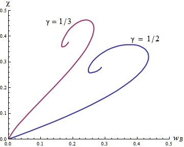
Eq. (81) leads to a well defined EoS for . For , the pressure becomes negative. In Fig. 6, we plot the spiral curve of regular solutions for and for (a value very close to ). The solutions almost coincide on the segment of the curve between the origin and , but they differ significantly at the metastable configurations.
Next, we apply the MEP to solutions of the TOV equation for . The corresponding Oppenheimer-Volkoff limit is . Again, we find that for , the MEP identifies regular solutions as equilibrium states and that for , equilibrium states are singular—see, Fig. 7. In Fig. 8, we plot the equilibrium entropy as a function of , and we find that the ratio is about 2.7.


C.2 Polytropic EoS
Next, we consider matter described by Gratton’s EoS [34]
| (82) |
where is a positive constant and . The EoS (82) is polytropic at low densities; where is the standard polytropic index. For large , the EoS describes ultra-relativistic particles. Note that, in general, may be a function of .
We define and with . Then, the EoS (82) becomes
| (83) |
By Eq. (55), for some constant . Pressure is well-defined only for . The EoS is thermodynamically consistent only if and vanish for . Thus, we express the EoS (82) as
| (84) |
where . (Note that the condition for the vanishing of the pressure is equivalent to the condition of Sec. 3.1, if we identify , where is the neutron mass. Then .)
We integrate the equations from the boundary inwards with boundary conditions and . For singular solutions, becomes unity at a finite distance from the singularity, so that for , . Then, we evaluate the singularity entropy
| (87) |
The free entropy (19) becomes , where
| (88) |
For , the EoS (84) at small describes non-relativistic free fermions. There is little qualitative difference from the EoS of free relativistic particles. We focus on smaller values of that lead to to regular solutions with higher compactness parameters. In Fig. 9, we plot the spirals of the regular solutions for and . The maximum masses are and , respectively. The application of the MEP leads to the same results: equilibrium states are regular solutions for and singular solutions for —see, Fig. 10. As shown in Fig. 11, the ratio is about for both values of .


C.3 MIT bag EoS
Next, we consider a toy EoS for quark matter that follows from an elementary version of the MIT bag model [35]. The model assumes massless and non-interacting quarks confined in a ‘bag’ that originates from the QCD vacuum. The confinement is described by the ‘bag constant’ that determines the energy difference between the standard and the QCD vacua.
The EoS is
| (89) | |||||
| (90) | |||||
| (91) |
where
| (92) |
and is the number of independent quark species. Eqs. (89—91) imply that , where . Positivity of pressure implies that vanishes for .
We write and in terms of the dimensionless temperature . Then, the EoS reads
| (93) |
The boundary of the star is defined by . This implies that and the temperature at infinity is .
We integrate the equations from the boundary inwards with boundary conditions and . For singular solutions, becomes unity at a finite distance from the singularity, so that for , . The free entropy (19) becomes , where
| (94) |
In Fig. 12, we plot the spiral curve of regular solutions. The maximum mass is found at . Again, we find that for , the MEP identifies regular solutions as equilibrium states and that for , equilibrium states are singular—see Fig. 13. In Fig. 14, we plot the free entropy of the equilibrium solutions as a function of and we find .


C.4 The asymptotic behavior of the EoS
Finding the conditions that an EoS must satisfy in order to be compatible with relativity is an old problem that has not yet been resolved. The causality condition is well accepted, since it guarantees that the speed of sound on the material never exceeds the speed of light. Other conditions have been suggested but they are not universally accepted. For example, Landau and Lifschitz proposed [36] that
| (95) |
This follows from the assumption that for sufficiently high energy all particles behave like massless particles even in presence of interactions. Counterexamples exist [37, 38]; however, theories characterized by asymptotic freedom are expected to satisfy (95) for .
Relativistic constraints to the EoS, other than causality, do not usually enter the compact-star models. Potential violations would typically appear at very high densities, well beyond the regime of physical interest. However, here we consider virtual solutions to the Einstein equations at extreme densities and far from thermodynamic equilibrium. In this regime, the asymptotic behavior of the EoS as is relevant.
In all examples that we have considered so far, the EoS satisfies Eq. (95). The free entropy remains finite as for fixed , the values of being much smaller than the global maximum. However, EoS with different asymptotic behavior leads to blowing up as . The equilibrium state corresponds to . Then, regular solutions are metastable states rather than equilibrium states. This is the case, for example, for the EoS of the non-relativistic free fermion gas with a causality-violating asymptotic behavior, .
The EoS for constants and does not violate causality. For , it describes the MIT bag model; for , it coincides with the EoS for the ‘most compact’ star considered in Ref. [39].
As in the model of Sec. E.3, a transition temperature appears as an integration constant. Writing , , and , the EoS becomes
| (96) | |||||
| (97) |
We define the dimensionless variables , and Then, Eqs. (2—4) coincide with Eqs. (85, 86), and the free entropy becomes , where
| (98) |
The implementation of the MEP for is shown in Fig. 15. Regular solutions still define local maxima of the free entropy, but these maxima are no longer global, because the free entropy diverges as . Matter with this EoS cannot form stable compact stars, because they have always less entropy from the black-hole-like configurations at . We find that this behavior persists for values of . For , we recover the results presented in the main text and in the previous sections.

There are two possible interpretations of this result. Either relativistic consistency implies Eq. (95) as (a result that remains to be proven from first principles), or matter that violates (95) exists but it cannot form stable compact stars.
Finally, we note that any EoS that is employed for neutron stars can also be employed for the study of singularity stars, as long as a high density cut-off is included so that Eq. (95) is enforced for all .
References
- [1] J. Katz and Y. Manor, Entropy Extremum of Relativistic Self-Bound Systems: A Geometric Approach, Phys. Rev. D12, 956 (1975).
- [2] N. Savvidou and C. Anastopoulos, The Thermodynamics of Self-gravitating Systems in Equilibrium is Holographic, Class. Quant. Grav. 31, 055003 (2014).
- [3] H. B. Callen, Thermodynamics and an Introduction to Thermostatistics (John Wiley, New York, 1985).
- [4] S. W. Hawking, The Path-Integral Approach to Quantum Gravity, in General Relativity: an Einstein Centenary Survey, edited by S. W. Hawking and W. Israel (Cambridge University Press, 1979).
- [5] G. W. Gibbons and S. W. Hawking, Action Integrals and Partition Functions in Quantum Gravity, Phys. Rev. D15, 2752 (1977).
- [6] R. M. Wald, Black Hole Entropy is Noether Charge, Phys. Rev. D48, 3427 (1993).
- [7] C. Anastopoulos and N. Savvidou, Entropy of Singularities in Self-Gravitating Radiation, Class. Quant. Grav. 29, 025004 (2012).
- [8] W. H. Zurek and D. N. Page, Black-hole Thermodynamics and Singular Solutions of the Tolman-Oppenheimer-Volkoff Equation, Phys. Rev. D29, 628 (1984).
- [9] C. Anastopoulos and N. Savvidou, The Thermodynamics of a Black Hole in Equilibrium Implies the Breakdown of Einstein Equations on a Macroscopic Near-Horizon Shell, JHEP 144 (2016).
- [10] H. C. Kim, Classifying Self-Gravitating Radiations, Phys. Rev. D 95, 044021 (2017).
- [11] J. Smoller and B. Temple, On the Oppenheimer‐Volkoff Equations in General Relativity, Arch. Rational Mech. Anal. 142, 177 (1998).
- [12] S. W. Hawking and G. R. F. Ellis, The Large Scale Structure of Spacetime (Cambridge University Press, Cambridge 1973).
- [13] R. P. Geroch, What is a Singularity in General Relativity?, Ann. Phys. (New York), 48, 526 (1968).
- [14] J. W. York, Role of Conformal Three-Geometry in the Dynamics of Gravitation, Phys. Rev. Lett. 28, 1082 (1972).
- [15] J. Kijowski, A. Smolski and A. Gornicka, Hamiltonian theory of Self-Gravitating Perfect Fluid and a Method of Effective Deparametrization of Einstein’s Theory of Gravitation, Phys. Rev. D 41, 1875 (1990).
- [16] J.R. Oppenheimer and G.M. Volkoff, On Massive Neutron Cores, Phys. Rev. 55, 374 (1939).
- [17] C. W. Misner, K. S. Thorne and J. A. Wheeler, Gravitation (W. H. Freeman and Co, 1973).
- [18] S. Yabushita, Pulsational Instability of Isothermal Gas Spheres within the Framework of General Relativity, Mon. Not. R. Astron. Soc. 165, 17 (1973).
- [19] R. J. Gleiser and G. Dotti, Instability of the Negative Mass Schwarzschild Naked Singularity, Class.Quant.Grav. 23, 5063 (2006).
- [20] S. Chandrasekhar, The Dynamical Instability of Gaseous Masses Approaching the Schwarzschild Limit in General Relativity, Phys. Rev. Lett. 12, 114 (1964).
- [21] G. T. Horowitz, Semiclassical Relativity: The Weak-Field Limit, Phys. Rev. D21, 1445 (1980).
- [22] P. R. Anderson, C. Molina-París, and E. Mottola, Linear Response, Validity of Semiclassical Gravity, and the Stability of Flat Space, Phys. Rev. D67, 024026 (2003).
- [23] B. L. Hu, A. Roura, and E. Verdaguer, Induced Quantum Metric Fluctuations and the Validity of Semiclassical Gravity, Phys.Rev. D70, 044002 (2004).
- [24] D. M. Eardley and Larry Smarr, Time Functions in Numerical Relativity: Marginally Bound Dust Collapse,Phys. Rev. D19, 2239 (1979).
- [25] D. Christodoulou, Violation of Cosmic Censorship in the Gravitational Collapse of a Dust Cloud, Commun. Math. Phys. 93, 171 (1984).
- [26] P. S. Joshi, Gravitational Collapse and Spacetime Singularities (Cambridge University Press, Cambridge 2007).
- [27] P. S. Joshi and D. Malafarina, Recent Developments in Gravitational Collapse and Spacetime Singularities, Int. J. Mod. Phys. D20, 2641 (2011).
- [28] P. S. Joshi, D. Malafarina, and R. Narayan, Equilibrium Configurations from Gravitational Collapse, Class. Quant. Grav. 28 235018 (2011).
- [29] P. S. Joshi, D. Malafarina, and R. Narayan, Dynamics of dissipative gravitational collapse, Class. Quantum Grav. 31 015002 (2014).
- [30] L. Herrera and N. O. Santos, Dynamics of Dissipative Gravitational Collapse, Phys. Rev. D70, 084004 (2004).
- [31] R. Penrose, Gravitational Collapse: the Role of General Relativity, Rivista del Nuovo Cim. Numero speciale 1, 252 (1969).
- [32] R. Penrose, Singularities and Time-Asymmetry, in Einstein Centenary Volume, S. W. Hawking and G. Ellis (eds.), (Cambridge University Press, 1979).
- [33] S. A. Chin and J. D. Walecka, An Equation of State for Nuclear and Higher-Density Matter Based on Relativistic Mean-Field Theory, Phys. Lett. 52B, 24 (1974).
- [34] L. Gratton, Rend. Accad. Nasionale dei Lincei 38, 354 (1964).
- [35] A. Chodos, R. L. Jaffe, K. Johnson, C. B. Thorn and V. F. Weisskopf, New Extended Model of Hadrons, Phys. Rev. D9, 3471 (1974).
- [36] L. D. Landau and E. M. Lifshitz, The Classical Theory of Fields, 4th edition (Pergamon Press, 1975), pg. 87.
- [37] Y. B. Zel’dovich, Equation of State at a Superhigh Density and Relativistic Restrictions, JETP 41, 1609 (1961).
- [38] R. P. Geroch and D. J. Hegyi, Relativistic Equations of State, Nature 215, 501 (1967).
- [39] S. Koranda, N. Stergioulas and J. L. Friedman, Upper Limits Set by Causality on the Rotation and Mass of Uniformly Rotating Relativistic Stars, Ap. J. 488, 799 (1997).