Exploiting Multi-layer Graph Factorization for
Multi-attributed Graph Matching

A single-layer graph matching problem finds correspondences between two attributed graphs that are described as single-layer structures. This includes not only single-attributed graph matching but also multi-attributed graph matching problems, because multiple attributes can be considered as a single attribute by integrating them.

For given two attributed graphs $\mathcal{G}_{1}$ and $\mathcal{G}_{2}$, this problem is commonly formulated as a Lawler’s quadratic assignment problem (QAP) [3, 6, 16, 24, 33]. Each graph $\mathcal{G}_{k}$ is defined as a set $\left\{\mathcal{V}_{k},\mathcal{E}_{k},\mathcal{A}_{k}\right\}$, where $\mathcal{V}_{k}$ is a set of vertices, $\mathcal{E}_{k}$ represents a set of edges, and $\mathcal{A}_{k}$ is a set of attributes that describe each vertex and edge. In the Lawler’s QAP formulation, the correspondences between two sets of vertices are represented using an $({N}_{1}\times{N}_{2})$-dimensional binary assignment matrix $\mathbf{X}$, where ${N}_{1}$ and ${N}_{2}$ represent the numbers of vertices in the graphs. Each element of the matrix $\left[\mathbf{X}\right]_{i,a}$ indicates a correspondence relation between ${v}_{(1)i}\in\mathcal{V}_{1}$ and ${v}_{(2)a}\in\mathcal{V}_{2}$. For example, if ${v}_{(1)i}$ and ${v}_{(2)a}$ are matched, $\left[\mathbf{X}\right]_{i,a}=1$, otherwise $\left[\mathbf{X}\right]_{i,a}=0$. On the other hand, the affinity information between two matching candidates is described using an $({N}_{1}{N}_{2}\times{N}_{1}{N}_{2})$-dimensional matrix $\mathbf{K}$. Each diagonal element of the matrix $\left[\mathbf{K}\right]_{ia,ia}$ describes a unary affinity of a matching candidate $\left({v}_{(1)i},{v}_{(2)a}\right)$, and each non-diagonal element $\left[\mathbf{K}\right]_{ia,jb}$ describes a pairwise affinity of two matching candidates $\left({v}_{(1)i},{v}_{(2)a}\right)$ and $\left({v}_{(1)j},{v}_{(2)b}\right)$. These affinity values are computed by using the vertex and edge attributes. Then, the graph matching problem can be formulated as follows:

where $\mathbf{1}_{N}$ is an $N$-dimensional all-ones vector, and the vector inequality constraints represent the one-to-one matching constraint of the graph matching problem. Since this QAP is a well-known NP-hard problem, previous works [3, 6, 16, 24, 33] addressed the problem by relaxing the binary matching constraint to find an approximated solution in the continuous domain.

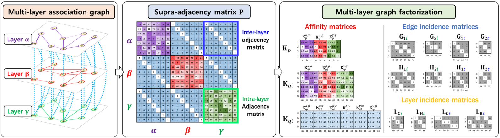
The formulation of multi-layer graph matching was firstly proposed in [24] to solve multi-attributed graph matching problems. They proposed a multi-layer association graph structure inspired by the multiplex network structure [7, 15, 25]. The graph $\mathcal{G}_{k}\left(\mathcal{V}_{k},\mathcal{E}_{k},\mathcal{A}_{k},\mathcal{L}_{k}\right)$ consists of multiple layers that describe multiple attributes respectively, and the layers are linked to each other as shown in Fig. 2. Here, $\mathcal{L}_{k}$ is a set of layer indices. In contrast to the single-layer structure, each vertex ${v}^{\alpha}_{(k)i}\in\mathcal{V}_{k}$ has a layer index $\alpha\in\mathcal{L}_{k}$. For this reason, vertices that have different layer indices, ${v}^{\alpha}_{(k)i}$ and ${v}^{\beta}_{(k)i}$, are differentiated from each other, even though they have the same vertex index. Accordingly, each edge ${e}^{\alpha;\beta}_{(k)i;j}\in\mathcal{E}_{k}$ is also defined with two layer indices. Thus, a four-dimensional affinity tensor $\mathbf{\Pi}$ is required to express the multi-layer association graph structure as described in [24]. $\mathbf{\Pi}$ consists of two types of affinity matrices (intra- and inter-layer), which are arranged as a two-dimensional structure according to layer indices. $\mathbf{\Pi}$ can be flattened to a two-dimensional block matrix as shown in Fig. 2, which is called the supra-adjacency matrix [7, 12, 24, 25]. Then, a multi-layer graph matching problem can be formulated as

where $\otimes$ indicates the Kronecker product, and $\mathbf{P}$ is a supra-adjacency matrix. $\mathbf{L}_{\mathbf{C}}$ is an ${N}_{L}$-dimensional vector that describes relative confidence values among attributes, and ${N}_{L}$ represents the number of layers. Details of the $\mathbf{L}_{\mathbf{C}}$ estimation are presented in Sec. 5.3. Although this multi-layer based formulation effectively resolves the oversimplification problem by preserving characteristics of each attribute, the scalability problem caused by the huge size of the supra-adjacency matrix comes to the fore in exchange. To solve this scalability problem, we propose a matrix factorization method that divides the huge multi-layer matrix into several small matrices. Details are presented in Sec. 4.

Before relaxing the objective function ${F}_{gm}\left(\mathbf{X}\right)$, we derive an equivalent objective function by substituting Eq. (3) into Eq. (2) as follows:

where $\mathbf{Y}$ and $\mathbf{Z}$ are the pairwise intra- and inter-layer indicator matrices, and $\circ$ is the Hadamard product. $\mathbf{K}_{qi}$ and $\mathbf{K}_{qt}$ can be divided again into $\mathbf{K}_{qi}=\mathbf{U}\mathbf{V}^{\top}$ and $\mathbf{K}_{qt}=\mathbf{S}\mathbf{T}^{\top}$ respectively by using any factorization method such as the singular value decomposition (SVD). By using the decomposed matrices, Eq. (4) can be reformulated as follows:

where $\mathbf{u}_{m}$, $\mathbf{v}_{m}$, $\mathbf{s}_{m}$, and $\mathbf{t}_{m}$ are ${m}^{th}$ column vectors of the factorized matrices $\mathbf{U}$, $\mathbf{V}$, $\mathbf{S}$, and $\mathbf{T}$ respectively.²² 2 A formula $tr\left({\left(\mathbf{u}{\mathbf{v}}^{\top}\right)}^{\top}\left(\mathbf{A}\circ\mathbf{B}\right)\right)=tr\left(\text{diag}\left(\mathbf{u}\right)\mathbf{A}\text{diag}\left(\mathbf{v}\right)\mathbf{B}^{\top}\right)$ is always satisfied for $\mathbf{u}\in\mathbb{R}^{m}$, $\mathbf{v}\in\mathbb{R}^{n}$ and $\mathbf{A},\mathbf{B}\in\mathbb{R}^{m\times n}$ [33]. $\mathbf{\Lambda}_{i}$ and $\mathbf{\Lambda}_{t}$ describe the confidence of each layer, and distribute the confidence information into intra- and inter-layer edges. $\mathbf{v}_{m,n}$ and $\mathbf{t}_{m,n}$ are ${n}^{th}$ block vectors that are extracted by separating $\mathbf{v}_{m}$ and $\mathbf{t}_{m}$ according to ${N}_{qi}^{L}$ and ${N}_{qt}^{L}$, which are the numbers of sub-matrices of intra- and inter-layer affinity matrices. $\left[\mathbf{\Lambda}_{i}\right]_{n,n}$ and $\left[\mathbf{\Lambda}_{t}\right]_{n,n}$ are ${n}^{th}$ diagonal terms of $\mathbf{\Lambda}_{i}$ and $\mathbf{\Lambda}_{t}$ respectively.

Given the reformulated objective function Eq. (5), we can derive convex and concave relaxations of the function similar to the single-layer factorized graph matching algorithm [33, 34] as follows:

where ${F}_{con}$ is a constant when $\mathbf{X}$ is a permutation matrix $(\emph{e.g}.\hbox{}~\mathbf{X}\mathbf{X}^{\top}=\mathbf{X}^{\top}\mathbf{X}=\mathbf{I})$. Since the Hessian of ${F}_{vex}\left(\mathbf{X}\right)$ with respect to $\text{vec}\left(\mathbf{X}\right)$ is always negative semidefinite, ${F}_{vex}\left(\mathbf{X}\right)$ of the maximization problem is a convex function. Similarly, since the Hessian of ${F}_{cav}\left(\mathbf{X}\right)$ is always positive semidefinite, ${F}_{cav}\left(\mathbf{X}\right)$ is a concave function. However, since $\mathcal{G}_{1}$ and $\mathcal{G}_{2}$ often have different sizes in practical application, $\mathbf{X}$ cannot satisfy the condition as a permutation matrix in general. To convert $\mathbf{X}$ to a permutation matrix, we add dummy nodes to the smaller graph as presented in [33, 34]. Details of the proof are presented in the supplementary materials.

The objective function of the proposed multi-layer path following algorithm can be constructed by combining two relaxed functions (Eq. (6) and Eq. (7)) as follows:

where $\theta$ is a control parameter that is gradually increased during the optimization process. We fixed the step size for increasing $\theta$ to 0.01 in all experiments. Based on this objective function, the multi-layer path following algorithm can be designed as shown in Algorithm 1. Since ${F}_{\theta}\left(\mathbf{X}\right)$ is a convex function at the start of the algorithm, we can find a global optimum by using convex optimization methods such as modified Frank-Wolfe (FW) algorithm [10]. During the series of iteration steps, ${F}_{\theta}\left(\mathbf{X}\right)$ is gradually changed to a concave function that has the same global optimum as the original objective function. At the same time, the optimum of ${F}_{\theta}\left(\mathbf{X}\right)$ also approaches the globally optimal solution.

In the middle of iteration steps (Lines 7-8), the path is modified based on the proposed layer confidence measure that evaluates relative confidences among attributes. This modification encourages the optimization algorithm to follow the information of more confident attributes. Details of the measure are presented in Sec. 5.3.

To define a layer confidence measure, we first assume that true correspondences have strong affinities with themselves, while false correspondences have relatively weak connections with others; because the correctly matched graphs should have similar structures. This assumption has been used frequently in recent works that follow the spectral matching scheme [3, 4, 6, 16]. Based on this, we use the difference between the connection strength of true/false clusters as a confidence measure because the difference is decreased when true/false clusters become jumbled.

The connection strength can be determined by computing the average affinity value of each cluster. However, since true correspondences are unidentified during the matching process, we temporally use the current solution as a true/false indicator matrix. Finally, the proposed layer confidence measure is defined as follows:

where $\mathbf{X}$ is a discretized current solution by using discretization methods such as the Hungarian method [22], and $\mathbf{\overline{X}}$ is the binary complement vector of $\mathbf{X}$.

As stated above, the multi-layer structure has a scalability problem caused by the huge size of the supra-adjacency matrix. The space requirements grow as $O\left({N}_{v}^{4}{N}_{L}^{2}\right)$, where ${N}_{v}$ is the number of vertices and ${N}_{L}$ is the number of layers. On the other hand, the proposed algorithm has fewer space requirements $O\left({N}_{v}^{4}{N}_{L}+{N}_{v}^{2}{N}_{L}^{2}\right)$. Since the number of attributes greatly affects the expressivity and robustness of the algorithm, the proposed factorization relieves the scalability problem when we increase the number of attributes. Moreover, because most matrix operations can be performed before starting the optimization process, the proposed algorithm can take advantage of the computational complexity aspect.

We evaluate the proposed algorithm for synthetic graph matching problems. To generate a pair of synthetic graphs, we use the same experimental scheme outlined in [24]. First, an initial graph $\mathcal{G}_{0}$ is generated, which has several types of attributes $\mathcal{A}_{0}$. To assign different characteristics into each attribute, we randomly generate attribute values with different variances for each layer. Then, we generate two graphs $\mathcal{G}_{1}$ and $\mathcal{G}_{2}$ by adding small attribute deformations that follow a Gaussian distribution $\mathcal{N}\left(0,{\epsilon}^{2}\right)$ and the same number of randomly defined outliers ${v}_{out}$ into $\mathcal{G}_{0}$. Each element of an intra-layer affinity matrix $\left[\mathbf{K}^{\alpha;\alpha}\right]_{ia,jb}$ is defined as follows:

where $\left[{r}^{\alpha}_{1}\right]_{ij}$ and $\left[{r}^{\alpha}_{2}\right]_{ab}$ are randomly assigned edge attributes of layer $\alpha$, and $\sigma$ is a scaling factor that is fixed as $0.3$ in these experiments. $\omega$ is a control parameter that determines the variance of the affinity values and reflects different characteristics of each attribute. $\omega$ is randomly selected in $[0.1,1]$. To integrate the attributes for single-layer graph matching algorithms, we normalize the affinity matrices individually and aggregate the matrices by summing them.

Then, we performed three types of experiments: deformation, outlier, and attributes, as listed in Table 2. In the deformation experiment, each pair of graphs is generated with different magnitudes of deformation $\epsilon$, while the other parameters are fixed. By contrast, in the outlier experiment, only the number of outliers ${N}_{out}$ is varied. In the last experiment, both of the parameters are fixed, and the number of attributes is varied. For all experiments, the number of inliers is fixed as 20, and each experiment is iteratively performed 100 times.

As shown in Fig. 3, the proposed algorithm (‘MLFGM-multi’) exhibits better performance than most of the other methods.⁴⁴ 4 The postfix ‘-single’, ‘-integrated’, and ‘-multi’ indicate the results obtained using a single attribute, an integrated attribute, and multiple attributes, respectively. Note that we only present the best result among all the ‘-single’ results for each method for comparison. Moreover, as stated in [24], this synthetic graph matching scheme cannot fully exploit practical environments that contain real attributes having complex properties. Thus, to evaluate our algorithm in realistic environments, we perform the second experiment using general real images in Sec. 6.2.

In this experiment, we use graphs that are constructed from real images in the WILLOW dataset [2] to evaluate the proposed algorithm in realistic environments. The WILLOW dataset consists of five classes: face, motorbike, car, duck, and winebottle, and provides annotations that reflect each object structure. To generate a graph from each image, we first extract interest points by using the Hessian detector [23]. Then, we select the 10 nearest interest points from the annotated points as inliers. To consider variations caused by deformation and outliers, we randomly select pairs of images for each category, and include outliers that are randomly selected among the remaining interest points. The number of outliers is varied from 0 to 10 for each category, and each test is iterated 100 times for each category.

We define four types of attributes as listed in Table 3. CSiD and CCoD are appearance attributes that describe each edge attribute by concatenating the SIFT descriptors [21] of two interest points and RGB color histograms respectively. The geometric attributes, RDHD and RAHD, are generated by separating the log-polar histogram of HARG [2] into relative distance and angle histograms. Then, we use the normalized Hamming distance [2] to compute differences between two attribute vectors, which are defined as affinity values. The affinity matrices are normalized again for each layer to adjust the scales among attributes. Finally, an integrated affinity matrix is constructed by summing the normalized matrices.

As shown in Table 4 and Fig. 4, the proposed algorithm exhibits state-of-the-art performance in all categories except the face category — our algorithm shows a relatively lower matching accuracy in the face category. This is because the proposed layer confidence measure fails when evaluating the confidence values more frequently than the other categories. Nevertheless, the proposed algorithm shows comparable performance to other algorithms in the category. We expect that the problem can be resolved by improving the measure using more sophisticated learning-based methods. We will address this issue in future work.

References

- [1] H.-T. Chen, H.-H. Lin, and T.-L. Liu. Multi-object tracking using dynamical graph matching. In Proceedings of IEEE Conference on Computer Vision and Pattern Recognition, 2001.
- [2] M. Cho, K. Alahari, and J. Ponce. Learning graphs to match. In Proceedings of IEEE International Conference on Computer Vision, 2013.
- [3] M. Cho, J. Lee, and K. M. Lee. Reweighted random walks for graph matching. In Proceedings of European Conference on Computer Vision, 2010.
- [4] M. Cho, J. Sun, O. Duchenne, and J. Ponce. Finding matches in a haystack: A max-pooling strategy for graph matching in the presence of outliers. In Proceedings of IEEE Conference on Computer Vision and Pattern Recognition, 2014.
- [5] D. Conte, P. Foggia, C. Sansone, and M. Vento. Thirty years of graph matching in pattern recognition. In International Journal of Pattern Recognition and Artificial Intelligence, 18(03):265–298, 2004.
- [6] T. Cour, P. Srinivasan, and J. Shi. Balanced graph matching. In Proceedings of Advances in Neural Information Processing Systems, 2006.
- [7] M. De Domenico, A. Solé-Ribalta, E. Omodei, S. Gómez, and A. Arenas. Centrality in interconnected multilayer networks. In arXiv preprint arXiv:1311.2906, 2013.
- [8] O. Duchenne, F. Bach, I.-S. Kweon, and J. Ponce. A tensor-based algorithm for high-order graph matching. In IEEE Transactions on Pattern Analysis and Machine Intelligence, 33(12):2383–2395, 2011.
- [9] O. Duchenne, A. Joulin, and J. Ponce. A graph-matching kernel for object categorization. In Proceedings of IEEE International Conference on Computer Vision, 2011.
- [10] M. Fukushima. A modified frank-wolfe algorithm for solving the traffic assignment problem. Transportation Research Part B: Methodological, 18(2):169–177, 1984.
- [11] S. Gold and A. Rangarajan. A graduated assignment algorithm for graph matching. In IEEE Transactions on Pattern Analysis and Machine Intelligence, 18(4):377–388, 1996.
- [12] S. Gomez, A. Diaz-Guilera, J. Gomez-Gardeñes, C. J. Perez-Vicente, Y. Moreno, and A. Arenas. Diffusion dynamics on multiplex networks. In Physical review letters, 110(2):028701, 2013.
- [13] C. Gomila and F. Meyer. Graph-based object tracking. In Proceedings of IEEE International Conference on Image Processing, 2003.
- [14] Q.-X. Huang, G.-X. Zhang, L. Gao, S.-M. Hu, A. Butscher, and L. Guibas. An optimization approach for extracting and encoding consistent maps in a shape collection. In ACM Transactions on Graphics, 31(6):167, 2012.
- [15] M. Kivelä, A. Arenas, M. Barthelemy, J. P. Gleeson, Y. Moreno, and M. A. Porter. Multilayer networks. In Journal of Complex Networks, 2(3):203–271, 2014.
- [16] M. Leordeanu and M. Hebert. A spectral technique for correspondence problems using pairwise constraints. In Proceedings of IEEE International Conference on Computer Vision, 2005.
- [17] M. Leordeanu, M. Hebert, and R. Sukthankar. An integer projected fixed point method for graph matching and map inference. In Proceedings of Advances in Neural Information Processing Systems, 2009.
- [18] Z.-Y. Liu and H. Qiao. GNCCP–graduated nonconvexity and concavity procedure. In IEEE Transactions on Pattern Analysis and Machine Intelligence, 36(6):1258–1267, 2014.
- [19] Z.-Y. Liu, H. Qiao, and L. Xu. An extended path following algorithm for graph-matching problem. In IEEE Transactions on Pattern Analysis and Machine Intelligence, 34(7):1451–1456, 2012.
- [20] Z.-Y. Liu, H. Qiao, X. Yang, and S. C. Hoi. Graph matching by simplified convex-concave relaxation procedure. In International Journal of Computer Vision, 109(3):169–186, 2014.
- [21] D. G. Lowe. Distinctive image features from scale-invariant keypoints. In International Journal of Computer Vision, 60(2):91–110, 2004.
- [22] J. Munkres. Algorithms for the assignment and transportation problems. In Journal of the Society for Industrial and Applied Mathematics, 5(1):32–38, 1957.
- [23] K. P. Murphy. Machine learning: a probabilistic perspective. MIT press, 2012.
- [24] H.-M. Park and K.-J. Yoon. Multi-attributed graph matching with multi-layer random walks. In Proceedings of European Conference on Computer Vision, 2016.
- [25] A. Solé-Ribalta, M. De Domenico, S. Gómez, and A. Arenas. Random walk centrality in interconnected multilayer networks. In arXiv preprint arXiv:1506.07165, 2015.
- [26] L. Torresani, V. Kolmogorov, and C. Rother. Feature correspondence via graph matching: Models and global optimization. In Proceedings of European Conference on Computer Vision, 2008.
- [27] L. Torresani, V. Kolmogorov, and C. Rother. A dual decomposition approach to feature correspondence. In IEEE Transactions on Pattern Analysis and Machine Intelligence, 35(2):259–271, 2013.
- [28] J. Xiao, H. Cheng, H. Sawhney, and F. Han. Vehicle detection and tracking in wide field-of-view aerial video. In Proceedings of IEEE Conference on Computer Vision and Pattern Recognition, 2010.
- [29] J. Yan, J. Wang, H. Zha, X. Yang, and S. Chu. Consistency-driven alternating optimization for multi-graph matching: a unified approach. In IEEE Transactions on Image Processing, 2015.
- [30] J. Yan, X.-C. Yin, W. Lin, C. Deng, H. Zha, and X. Yang. A short survey of recent advances in graph matching. In Proceedings of ACM International Conference on Multimedia Retrieval, 2016.
- [31] M. Zaslavskiy, F. Bach, and J.-P. Vert. A path following algorithm for the graph matching problem. In IEEE Transactions on Pattern Analysis and Machine Intelligence, 31(12):2227–2242, 2009.
- [32] Z. Zhang, Q. Shi, J. McAuley, W. Wei, Y. Zhang, and A. Van Den Hengel. Pairwise matching through max-weight bipartite belief propagation. In Proceedings of IEEE Conference on Computer Vision and Pattern Recognition, 2016.
- [33] F. Zhou and F. De la Torre. Factorized graph matching. In Proceedings of IEEE Conference on Computer Vision and Pattern Recognition, 2012.
- [34] F. Zhou and F. De la Torre. Deformable graph matching. in Proceedings of IEEE Conference on Computer Vision and Pattern Recognition, 2013.