k-FFNN: Using a priori knowledge in Feed-forward Neural Networks
Abstract
Recurrent neural network (RNN) are being extensively used over feed-forward neural networks (FFNN) because of their inherent capability to capture temporal relationships that exist in the sequential data such as speech. This aspect of RNN is advantageous especially when there is no a priori knowledge about the temporal correlations within the data. However, RNNs require large amount of data to learn these temporal correlations, limiting their advantage in low resource scenarios. It is not immediately clear (a) how a priori temporal knowledge can be used in a FFNN architecture (b) how a FFNN performs when provided with this knowledge about temporal correlations (assuming available) during training. The objective of this paper is to explore k-FFNN, namely a FFNN architecture that can incorporate the a priori knowledge of the temporal relationships within the data sequence during training and compare k-FFNN performance with RNN in a low resource scenario. We evaluate the performance of k-FFNN and RNN by extensive experimentation on MediaEval 2016 audio data (“Emotional Impact of Movies” task). Experimental results show that the performance of k-FFNN is comparable to RNN, and in some scenarios k-FFNN performs better than RNN when temporal knowledge is injected into FFNN architecture. The main contributions of this paper are (a) fusing a priori knowledge into FFNN architecture to construct a k-FFNN and (b) analyzing the performance of k-FFNN with respect to RNN for different size of training data.
{d.harsha,rupayan.chakraborty,sunilkumar.kopparapu}@tcs.com
Index Terms: Neural network, feedforward architecture, temporal knowledge, recurrent neural network, audio emotion
1 Introduction
Artificial neural networks are extensively used in all types of classification problems [1]. Speech technologies and applications are not exception to that. Subsequent advancements in the field of neural networks was adapted to build better speech processing systems [2]. Recurrent neural network (RNN) is one such advancement in neural networks, which is being used extensively to solve various problems in speech processing [3, 4]. Among those, audio (speech) emotion recognition is one of the latest developments which is an integral part of Human Computer Interaction (HCI) system. RNN has been successfully applied in speech emotion recognition [5].
(a) (b)
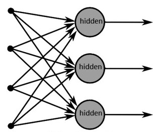
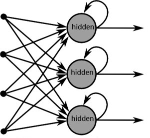
It is evident that a feed-forward neural network (FFNN) discriminatingly learns the patterns within the inputs, even from a low resource dataset [6]. But they are not designed to learn sequential relationships within the data. On the other side, deep neural networks like RNN has an inherent characteristic of learning and exploiting temporal relationships amongst the sequences [7, 8, 9], however RNN requires large training data to capture those correlations. Figure 1(a) shows the general architecture of a FFNN and Figure 1(b) shows the structure of a RNN. The essential difference between the two is the self loop within the hidden layer which is useful in capturing the unseen temporal relationship that might exist in the training data. The general structure of an FFNN as shown in Figure 1(a), consists of three layers i.e., input layer, hidden layer and output layer. The input data or features are fed to the input layer which pass through the hidden layer to the output layer. Here the input features or the posterior probabilities pass from the input layer to the hidden layer and then to the output layer but never in backward direction. Hence, the name feed-forward neural network. In a FFNN, a mapping is obtained between the input features and the output values in a supervised learning condition. By design in FFNN, no information regarding the sequence in which the inputs are fed to the network is captured. In FFNN, all the input data sequences are considered independent of each other. On the other hand a RNN network (see Figure 1(b)) is similar to FFNN except for the feedback loop in the hidden layer. This ensures the capture of temporal information in the sequence of inputs along with the mapping between the input and output is also captured.
In this paper we explore the use of knowledge regarding the temporal relationships within the sequence of training data while using a FFNN architecture for a limited resource scenario. Knowing that an RNN architecture is capable of inherently learning the temporal relationships that exist in the sequential data, we use RNN to automatically capture that information. However, this aspect of RNN is useful especially when there is no a priori knowledge about the temporal correlations within the data. But to learn temporal correlations automatically, substantial amount of training data are required.
What if a priori knowledge of the temporal relationships within the data sequences are known for limited samples, can a FFNN perform similar as an RNN?
In this work, a FFNN architecture which can use a priori knowledge of temporal correlationships has been explored, and we call it k-FFNN (short form of knowledge infused FFNN). In particular, we capture the relationship between FFNN and RNN, and then subsequently show through extensive experiments that the knowledge of temporal relationship can be infused to improve the performance of FFNN in a way that resembles RNN. Using MediaEval 2016 audio data (“Emotional Impact of Movies” task)[10]), we conduct several experiments to establish that the performance of k-FFNN is comparable to RNN and in some scenarios k-FFNN outperform RNN. The main contributions of the paper are (a) incorporation of a priori temporal/sequential knowledge in FFNN to construct a k-FFNN and (b) experimentally showing that not only the performance of k-FFNN is as good as RNN, but also better when there is small amount of training data. The paper is organized as follows. Section 2 presents the hypothesis we make with some theoretical representations. In Section 3, we discuss the dataset used to validate our hypothesis. Section 4 describes the experiments conducted with an analysis. We conclude in Section 5.
2 Hypothesis
We start off with the hypothesis
FFNN infused with prior knowledge about temporal relationship between data is similar to RNN in terms of performance
As seen in Figure 1 the primary difference between an RNN and a FFNN is the presence of the hidden layer feedback self loop in RNN which adds memory to the RNN network over time. The question that we are addressing is if a regular FFNN fed with the sequence based a priori knowledge (i.e. k-FFNN) can perform as well as an RNN. In other words, if we had some a priori knowledge about the sequence can we use it without depending on RNN to learn it through its hidden layer feedback loop. This is very useful especially in the scenarios where the training data is sparse plus when we are aware of the sequential relationship between data a priori. We validate the hypothesis that the performance of k-FFNN and RNN are similar through an extensive experimentation using the MediaEval dataset.
2.1 Background
We validate our hypothesis by considering a simple network configuration and derive a set of expressions that show the relationship between k-FFNN and RNN. For sake of simplicity, we consider a (input-hidden-output nodes) network configuration. Additionally, we consider a data sequence of length 3. Consider the data shown in Table 1.
| Input | Output | ||
|---|---|---|---|
More elaborately, if each was of dimension then we would have Table 2 used as the input-output data to train RNN. We assume that there exists some temporal relationship between , , and , , , which can be captured as shown in Table 3 . Namely, the output associated with , , is actually , , instead of , , . This is the mode in which the a priori temporal knowledge existing between , , is infused into the training set. Note that a FFNN that uses training data as shown in Table 3 is what we call k-FFNN.
| Input | Output | |||
|---|---|---|---|---|
| - | ||||
| - | ||||
| - | ||||
| - | ||||
| Input | Output | |||
|---|---|---|---|---|
For a k-FFNN configuration, the model would be represented by a total of variables that represent the network. Namely, the weights connecting the input to the hidden layer and . While in case of RNN the model consists of not only the weights connecting the input to the hidden layer and the weights connecting the hidden and the output layer but also the feedback connection between the hidden layers. So in case of RNN, it is modeled by variable. The input data remaining the same, the differences in k-FFNN and RNN is captured in Table 4.
| Label | k-FFNN () | RNN () |
|---|---|---|
| Weights | - | |
| Output | - |
Assuming the same initial weights for both k-FFNN and RNN, we elaborate the process of how the weights (or the model) gets updated as it is trained. We assume the usual back-propagation based weights update.
In case of FFNN (see Figure 2), the output of the hidden node is given by
| (1) |
assuming the sigmoid to be the squashing transfer function and is the input and is a constant which determines the steepness of the sigmoid. Similarly the output would be
| (2) |
Now the error
| (3) |
is used to modify the weights () such that when the same input is given to k-FFNN it would reduce (called back propagation of error) generally using the steepest descent algorithm. The weight, for and the weight, for , for the hidden layer are modified as
| (4) |
where
| (5) |
| (6) |
The next input, namely , is passed through the network to obtain (1) and (2). Now is used to compute the error (3) followed by weight update (4). This continues for other inputs (Table 3) as shown in Algorithm 1 to complete an epoch. Generally the update happen over several epochs.
2.2 RNN
In RNNs, length of the input sequence (here ) apart from the values of the input sequence at each time instant is considered to train the networks. The output of the hidden layer in case of RNNs is given as
| (7) |
The output of RNN is given by
| (8) |
The error in the output estimation is
| (9) |
The error is backpropagated through the length of the sequence i.e., back propagation through time (BPTT) is used to modify the weights of RNN.
The weight modification of RNNs in general is
| (10) |
and
| (11) |
where is the activation function at the unit. So the weight modification for the output layer units is:
| (12) |
where
In the network architecture considered for this analysis, the output is available only at is an example. The weight modification at output layer gets modified as
| (13) |
The modification of the input to hidden layer weights is obtained as
| (14) |
and the recursive/hidden weights are modified as
| (15) |
here sigmoid activation function is considered for the hidden layers where is generally defined as
| (16) |
For the network architecture considered, the above equation gets modified as
| (17) |
and
| (18) |
So the weights are modified as
| (19) |
3 Working scenario and Dataset preparation
MediaEval 2016 dataset published for emotional impact of movies task is used in our analysis [10]. This dataset is part of the LIRIS-ACCEDE dataset [11, 12] and consists of video clips of duration - seconds which have been annotated by viewers for their perceived emotion, in terms of arousal and valance. Note that the perceived emotion annotation is for the entire video clip in terms of valance and arousal value in the range .
In this paper, to test our hypothesis, the problem of predicting the perceived valence (arousal) value of the viewer after watching the video is considered. Note that, as shown in Figure 3 the valence (arousal) value represent the emotional state of the viewer after having watched the video. It is not immediately clear if the perceived emotion annotated by the viewer is something that is perceived uniformly for the entire duration of the video clip or if the perceived emotion is based on a smaller segment which is the subset of the video clip. According to the [13, 12], each video clip in the dataset has a fade in at the beginning of the video clip and and a fade out at the end of the video clip. This implies that there is a priori knowledge in terms of how the emotion has a temporal relationship within the video clip. This aspect, namely the perceived emotion of a video clip has a fade in and fade out and is not uniform for the entire duration of the video clip motivates us to use MediaEval 2016 dataset to evaluate our hypothesis.
We created a dataset of smaller second video clips by segmenting the original video clip. Namely, a second original video clip produced second video clips, we retained the temporal relationship between the smaller video clips and the original video clip by naming the video clips appropriately. This enables us to incorporate the temporal correlations, in terms of the fade in and fade out, between the segments to test our hypothesis as mentioned in Section 2.

In our experiments we concentrate only on the audio obtained from video clips as the input and the corresponding annotated valence (arousal) values are the desired output. For testing the hypothesis, we first extracted the audio from the original video clip and then segmented the audio into smaller non-overlapping second duration, so a movie clip of seconds () duration, resulted in audio clips each of second duration. For example, if is the audio extracted from the original video then,
| (20) |
where represents the concatenation of the audio for . Note that there is a temporal relationship between ’s because they are in a time sequence and are from a single video clip. This construction (20) helps us in building a dataset that can be used to analyze our hypothesis, namely, a FFNN infused with temporal knowledge can work as well as a RNN in terms of its overall performance when used for predicting the estimated emotion of a movie clip.
Let be the input output pair; where can be either valence () or arousal () associated with the audio . As seen in Figure 4) the audio is made up of the audio sequence. So for a RNN we have the input as while the output is the associated (or ). However, since the input are temporally related, we assumed that the perceived valence (or arousal ) has a bearing on . Namely,
| (21) |
For example, could be a linear function,
such that and . Then each of the audio clips can be assigned a valence namely, , , , . Note that captures the known a priori temporal knowledge.

We use or equivalently to train RNN while we use , , , to train a FFNN. Notice that for both FFNN and RNN the input data is the same while the output in case of RNN is known (), we construct using the prior knowledge for use in FFNN.
4 Experimental Validation
In all our experiments, we used the audio extracted from video clips (MediaEval database) each of around () seconds duration [14]. The database has a valence (and arousal) value in the range for all the videos, namely for is available. We constructed each of second duration from of second duration for (see (20)). For each we extracted 384 features, which were used for Interspeech 2009 Emotion Challenge [15] using the openSMILE toolkit [16]. We used WEKA Toolkit [17] to reduce the feature dimension to using feature selection method.
If represent the extracted features from then the dataset used in our experiments for RNN training is shown in Table 5, and for FFNN set of experiments we constructed as mentioned in (21) resulting in a dataset as shown in Table 6. We used a variety of ’s to capture fade-in and fade-out in our experiments as shown in Table 7.
| Input | Output | |||
|---|---|---|---|---|
| Input | Output | Input | Output | Input | Output | |
|---|---|---|---|---|---|---|
| - | - | - | - | Type | ||||||
|---|---|---|---|---|---|---|---|---|---|---|
| 1 | 1 | 1 | 1 | 1 | 1 | 1 | 1 | 1 | 1 | FFNN |
| 0.75 | 0.9 | 1 | 1 | 1 | 1 | 1 | 1 | 0.9 | 0.75 | Fn1 |
| 0.3 | 0.6 | 1 | 1 | 1 | 1 | 1 | 1 | 0.6 | 0.3 | Fn2 |
| 0.1 | 0.2 | 1 | 1 | 1 | 1 | 1 | 1 | 0.2 | 0.1 | Fn3 |
4.1 Experimental Analysis

The performance of the proposed k-FFNN system is compared with the popular RNN architecture i.e., simple RNN, RNN with Long-short-term-memory (LSTM) units and bi-directional RNN with LSTM (BLSTM) units). In this analysis, all k-FFNN and RNN systems are implemented using Keras deep learning toolkit [18]. The architectures of the systems considered in this analysis are shown in Table 8. For all systems, only a single hidden layer is considered. The hidden layer size is selected by varying the number of units from 11 (half of the sum of number of input (i.e., 21) and output units (i.e., 1)) to 44 (twice the sum of number of input and output units) and selecting the number of nodes in the hidden layer which results in the best performance. Sigmoid (S in Table 8) is used as the non-linear activation function on the hidden units. The input layer has 21 linear (L) units and the output layer has a single linear (L) unit.
| Model Name | Architecture |
|---|---|
| k-FFNN (Fn1) | 21L 21S 1L |
| k-FFNN (Fn2) | 21L 21S 1L |
| k-FFNN (Fn3) | 21L 21S 1L |
| FFNN | 21L 22S 1L |
| RNN | 21L 21S 1L |
| LSTM | 21L 21S 1L |
| BLSTM | 21L 21S 1L |
The system performance is evaluated in terms of Mean Squared Error (MSE) and Pearson Correlation Coefficient (PCC). PCC along with MSE is used as a performance metric as PCC provides a better evaluation of the performance of the systems trained on datasets with output values arousal) distributed as shown in Figure 5. It can be observed from Figure 5 that the output values for arousal are concentrated more at a single value (at 1.5) compared to other values. For the considered metrics, lower the MSE values better is the performance of the system and higher the PCC values, better is the performance of the system.
The MSE and PCC values are computed at audio clip level for all the systems (k-FFNN and RNNs) to evaluate the performance. In case of RNNs, single output value is obtained for the given audio clip () containing the sequence . Subsequently, the computation of MSE and PCC is straight forward in case of RNNs. In case of a k-FFNN system (as shown in Table 6), for each subsegment corresponding to the audio clip , arousal/valence value are generated. To compute the MSE and PCC values for each audio clips , the output values obtained for each clips are scaled with a value depending on the function selected during training. Then the mean of the values obtained at all subsegments is computed and compared with the original value assigned to that audio clip to obtain the MSE and PCC values. If , , , , are the output obtained for all the audio segment corresponding to the audio clip , then
| (22) |
is the defined arousal/valence value of the audio clip .
The MSE and PCC values obtained by considering training sets of different sizes are shown in Figure 6 and Figure 7, respectively for different systems. It can be observed from Figure 6 that the MSE values obtained for k-FFNN (Fn1) is always lower or equal to that of the MSE values obtained for RNNs for all sizes of training set. k-FFNN system performs much better than RNN systems for smaller training dataset. It can be observed that there is a performance improvement of 0.05 (MSE) when 200 training samples are used. Note that the MSE of RNN is 0.977 compared to MSE of 0.927 for k-FFNN (for 200 training samples) with function Fn1. However the performance of k-FFNN closer to that of RNN when 6814 (90% of dataset) samples are used for training. The MSE values are lower for FFNN compared to RNN for smaller training sets but are higher when the training set size is increased (MSE is 0.940 for FFNN and 0.953 for RNN when 500 samples are considered and 0.847 for FFNN and 0.820 for RNN when 6814 samples are considered). This shows that the performance of k-FFNN in terms of MSE is better than FFNN and RNN, especially for smaller training set.

It can be observed from Figure 7 that the PCC values are consistently higher for k-FFNN when compared to RNNs. Similar to MSE, the variation in PCC values between k-FFNN and RNN is larger for smaller training sets (difference = 0.08 (0.079 for RNN and 0.16 for Fn1) when 200 train samples are considered) and gradually decreases when the size of the training set is increased (difference = 0.048 (0.226 for RNN and 0.274 for k-FFNN), when 6814 train samples are considered). The PCC values obtained for FFNN are lower compared to k-FFNN for all sizes of training set. The PCC values are higher for FFNN compared to RNNs for smaller training sets but are lower when size of the training set is increased (PCC is 0.093 for FFNN and 0.079 for RNN when 200 samples are considered and 0.191 for FFNN and 0.226 for RNN when 6814 samples are considered).

Table 10 shows the MSE and PCC values obtained on arousal values by considering different knowledge infused functions (shown in Table 7) to represent the temporal information. It can be observed from Table 9 that the performance of the k-FFNN system trained by considering Fn1 performs better than the systems trained using Fn2 and Fn3 (both in terms of MSE and PCC). It is to be observed that the performance of the k-FFNN systems developed by considering Fn2 and Fn3 is lower than FFNN. This shows that choosing a proper function (knowledge of sequential temporal correlations between data) to represent the temporal information is critical for the performance of the k-FFNN and any arbitrary function used to represent the temporal information will not improve the performance of k-FFNN but may even degrade the performance.
| Function | MSE | PCC |
|---|---|---|
| Fn1 | 0.820 | 0.274 |
| Fn2 | 0.871 | 0.185 |
| Fn3 | 1.55 | 0.059 |
Table 10 shows the MSE and PCC values obtained for the task of estimating the valence values for different systems. The MSE and PCC values are listed for systems trained on 6814 utterances. It can be observed that the performance of k-FFNN system (using Fn1) is better than RNN and FFNN systems. But the performance of k-FFNN systems (using Fn2 and Fn3) are lower than RNN and even FFNN. Hence the observations made from the prediction of arousal values is further supported by the results obtained for prediction of valence values.
| System | MSE | PCC |
|---|---|---|
| k-FFNN (Fn1) | 0.319 | 0.128 |
| k-FFNN (Fn2) | 0.454 | 0.029 |
| k-FFNN (Fn3) | 0.762 | -0.051 |
| RNN | 0.331 | 0.126 |
| LSTM | 0.327 | 0.124 |
| BLSTM | 0.329 | 0.122 |
| FFNN | 0.343 | 0.106 |
5 Conclusions
FFNN architecture does not consider the temporal relationship that exits in a data sequence as in case of a speech signal. RNN architecture by its design is able to implicitly learn the temporal correlations that exists between the data sequence. While RNNs are advantageous when (a) one is not explicitly aware of the temporal relationship between the sequential data and (b) when there is a large amount of training data. In this paper, we address the scenario when there is insufficient training data and when a priori temporal knowledge about the training data is explicitly known.
In this paper, we have shown how one can infuse explicitly known a priori temporal knowledge about the sequential data to enhance the performance of FFNN architecture. We first compared the differences between a simple RNN and a FFNN and showed that the a priori knowledge can in some sense compensate for the hidden layer feedback weights that contribute in capturing temporal relationship in the training data. This observation, leads us to construct k-FFNN, a knowledge infused FFNN which exploits the known a priori sequential knowledge in the training data. This is one of the main contributions of this paper. Based on this observation, we hypothesized that k-FFNN performs as well as an RNN because k-FFNN are able to infuse known knowledge in the data sequence into its architecture. We further showed, experimentally, that the performance of k-FFNN especially for smaller training datasets exceeds the performance of RNN both in terms of the MSE and PCC and the performance of both k-FFNN and RNN level out when amount of training data increases. These experiments validate the hypothesis FFNN infused with prior knowledge about temporal relationship between data is similar to RNN in terms of performance. The essential contribution of this paper is the incorporation of known knowledge, when available, to learn a FFNN without depending on a deep architecture like RNN that requires more samples for better training.
References
- [1] Teuvo Kohonen, “An introduction to neural computing,” Neural Networks, vol. 1, no. 1, pp. 3 – 16, 1988.
- [2] G. Hinton, L. Deng, D. Yu, G. E. Dahl, A. r. Mohamed, N. Jaitly, A. Senior, V. Vanhoucke, P. Nguyen, T. N. Sainath, and B. Kingsbury, “Deep neural networks for acoustic modeling in speech recognition: The shared views of four research groups,” IEEE Signal Processing Magazine, vol. 29, no. 6, pp. 82–97, Nov 2012.
- [3] A. Graves, A. r. Mohamed, and G. Hinton, “Speech recognition with deep recurrent neural networks,” in 2013 IEEE International Conference on Acoustics, Speech and Signal Processing, May 2013, pp. 6645–6649.
- [4] Alex Graves and Navdeep Jaitly, “Towards end-to-end speech recognition with recurrent neural networks.,” in ICML, 2014, vol. 14, pp. 1764–1772.
- [5] Felix Weninger, Fabien Ringeval, Erik Marchi, and Björn W. Schuller, “Discriminatively trained recurrent neural networks for continuous dimensional emotion recognition from audio,” in Proceedings of the Twenty-Fifth International Joint Conference on Artificial Intelligence, IJCAI 2016, New York, NY, USA, 9-15 July 2016, 2016, pp. 2196–2202.
- [6] Simon Haykin, Neural Networks: A Comprehensive Foundation (3rd Edition), Prentice-Hall, Inc., Upper Saddle River, NJ, USA, 2007.
- [7] David E. Rumelhart, Geoffrey E. Hinton, and Ronald J. Williams, “Neurocomputing: Foundations of research,” chapter Learning Representations by Back-propagating Errors, pp. 696–699. MIT Press, Cambridge, MA, USA, 1988.
- [8] Paul J. Werbos, “Generalization of backpropagation with application to a recurrent gas market model,” Neural Networks, vol. 1, no. 4, pp. 339 – 356, 1988.
- [9] Jeffrey L. Elman, “Finding structure in time,” Cognitive Science, vol. 14, no. 2, pp. 179–211, 1990.
- [10] “The 2016 emotional impact of movies task,” http://www.multimediaeval.org/mediaeval2016/emotionalimpact/index.html, 2016.
- [11] “Liris-accede database,” http://liris-accede.ec-lyon.fr/database.php, 2016.
- [12] Y. Baveye, E. Dellandréa, C. Chamaret, and L. Chen, “Liris-accede: A video database for affective content analysis,” IEEE Transactions on Affective Computing, vol. 6, no. 1, pp. 43–55, 2015.
- [13] Y. Baveye, E. Dellandréa, C. Chamaret, and L. Chen, “From crowdsourced rankings to affective ratings,” in 2014 IEEE International Conference on Multimedia and Expo Workshops (ICMEW), 2014, pp. 1–6.
- [14] “Mediaeval 2016 proceedings,” http://ceur-ws.org/Vol-1739/MediaEval_2016_paper_6.pdf, 2016.
- [15] Björn W. Schuller, Stefan Steidl, and Anton Batliner, “The INTERSPEECH 2009 emotion challenge,” in INTERSPEECH, 2009, pp. 312–315.
- [16] openSMILE, ,” http://www.audeering.com/research/opensmile, 2014.
- [17] Toolkit WEKA, ,” http://www.cs.waikato.ac.nz/ml/weka/, 2016.
- [18] “François chollet ”keras”,” https://github.com/fchollet/keras/, 2015.