跳到论文正文
W Papers独立论文阅读器 arXiv:1704.07035 论文正文 计算阅读时间 · 0%
引用这篇论文根据当前论文元数据生成,正式投稿前建议核对。


License: arXiv.org perpetual non-exclusive license
arXiv:1704.07035v2 [math-ph] 25 Oct 2017

Elliptic supersymmetric integrable model
and multivariable elliptic functions

Kohei Motegi ††thanks: E-mail: kmoteg0@kaiyodai.ac.jp Affiliation: Faculty of Marine Technology, Tokyo University of Marine Science and Technology, Affiliation: Etchujima 2-1-6, Koto-Ku, Tokyo, 135-8533, Japan
August 24, 2026
Abstract

We investigate the elliptic integrable model introduced by Deguchi and Martin, which is an elliptic extension of the Perk-Schultz model. We introduce and study a class of partition functions of the elliptic model by using the Izergin-Korepin analysis. We show that the partition functions are expressed as a product of elliptic factors and elliptic Schur-type symmetric functions. This result resembles the recent works by number theorists in which the correspondence between the partition functions of trigonometric models and the product of the deformed Vandermonde determinant and Schur functions were established.

1 Introduction

In statistical physics and field theory, integrable models [1, 2, 3, 4] play special roles not only because many physical quantities can be computed exactly but also because of its deep connections with mathematics. One of the highlights is the discovery of quantum groups [5, 6] through the investigations of the algebraic structure of the RR-matrix. From the point of view of integrable models, quantum groups are related with trigonometric models whose matrix elements are given in terms of trigonometric functions. There is also a class of elliptic integrable models whose matrix elements are given in terms of elliptic functions. The most famous one is the Baxter’s eight-vertex model [7]. Investigating the underlying algebraic structures, several versions of the elliptic quantum groups have been formulated and studied [8, 9, 10, 11, 12].

In statistical physics, the most important objects are partition functions. Partition functions of integrable models are global objects constructed from RR-matrices. By developing various methods such as the quantum inverse scattering method, there are now extensive studies on the partition functions of the elliptic eight-vertex solid-on-solid model [13, 14, 15, 16, 17, 18, 19, 20, 21], ranging from the domain wall boundary partition functions to the wavefunctions.

The elliptic model we mentioned above is the eight-vertex solid-on-solid model which is related with the Baxter’s eight-vertex model by the vertex-face transform. In this paper, we investigate another type of elliptic integrable model, which was introduced by Deguchi and Martin [22]. Deguchi and Martin introduced this elliptic model as an elliptic extension of the Perk-Schultz model [23]. The Perk-Schultz model is a trigonometric model, which was later found to have the quantum superalgebra structure [24]. Hence we sometimes call the Perk-Schultz model as supersymmetric integrable model.

The Deguchi-Martin model was constructed as an elliptic generalization of the face-type version of the Perk-Schultz model. The quantum supergroup structure seems not to be explored till now. For the case of the ordinary elliptic model, the elliptic quantum group structure is understood to be obtained by twisting the quantum group associated with the trigonometric models [12]. It might be possible to understand the underlying algebraic structure of the Deguchi-Martin model as an elliptic quantum supergroup obtained from a quasi-Hopf twist of the quantum supergroup of the trigonometric Perk-Schultz model.

The main motivation for studying elliptic versions of supersymmetric models in this paper comes from the previous works on the trigonometric version of the model. In recent years, trigonometric models were found to have connections with the field of algebraic combinatorics. Number theorists Bump-Brubaker-Friedberg [25] found that a class of partition functions of a free-fermion model in an external field gives rise to an integrable model realization of the Tokuyama formula for the Schur functions [26] (see also [27, 28, 29] for pioneering works on variations of the Tokuyama formula). Tokuyama formula is a one-parameter deformation of the Weyl character formula for the Schur functions. This fundamental result lead people to find generalizations and variations of the Tokuyama-type formula for various types of symmetric functions [30, 31, 32, 33, 34, 35, 36, 37, 38]. The latest topic is the introduction of the notion of the metaplectic ice, which is explicitly constructed in [36] by twisting the higher rank Perk-Schultz model.

As for the domain wall boundary partition function, the celebrated Izergin-Korepin analysis [39, 40] was performed, and factorization phenomena on the domain wall boundary partition functions was found for the Perk-Schultz model and the closely related Felderhof free-fermion model [41] in [42, 43] (see also [44] for an application to correlation functions). This factorization formula for the domain wall boundary partition functions cannot be observed in general for the case of the Uq​(s​l2)U_{q}(sl_{2}) six-vertex models. Instead, a determinant formula called as the Izergin-Korepin determinant was already obtained in 1980s [39, 40]. The factorization phenomena for the Perk-Schultz and Felderhof models was extended to the elliptic models [45, 46]. For example, an extensive study on the domain wall boundary partition functions of the Deguchi-Martin model was performed in the PhD thesis of Zuparic [46].

In this paper, focusing on the Deguchi-Martin model, we introduce and investigate the explicit forms of a more general class of partition functions which includes the domain wall boundary partition functions as a special case. We apply the Izergin-Korepin technique to study the partition functions which was recently applied to the Uq​(s​l2)U_{q}(sl_{2}) six-vertex model in [47].

By using the Izergin-Korepin technique, We prove that the partition functions are expressed as a certain multivariable elliptic functions. Let us briefly present this main result of this paper in some more detail. We denote the partition functions of the Deguchi-Martin model treated in this paper as WM,N(u1,…,uN|v1,…,vM|x1,…,xN|a12)W_{M,N}(u_{1},\dots,u_{N}|v_{1},\dots,v_{M}|x_{1},\dots,x_{N}|a_{12}). The precise definition will be given in Definition 2.2 in section 2. The partition functions are defined using the local elliptic weights of the Deguchi-Martin model, and are determined by the boundary conditions. Since the local weights of the Deguchi-Martin model will be described using spectral parameters and the state vectors, the partition functions depend on two classes of complex parameters u1,…,uNu_{1},\dots,u_{N}, v1,…,vMv_{1},\dots,v_{M} coming from the spectral parameters, and a complex parameter a12a_{12} coming from the state vectors. The partition functions we investigate in this paper also have dependence on boundary conditions, which are labelled using a sequence of integers x1,…,xNx_{1},\dots,x_{N} satisfying 1≤x1<⋯<xN≤M1\leq x_{1}<\cdots<x_{N}\leq M. The dependence on these parameters are why we denote the partition functions as WM,N(u1,…,uN|v1,…,vM|x1,…,xN|a12)W_{M,N}(u_{1},\dots,u_{N}|v_{1},\dots,v_{M}|x_{1},\dots,x_{N}|a_{12}).

The main result of this paper is Theorem 4.2 in section 4, which states that the partition functions is expressed as a product of elliptic factors and an elliptic version of the Schur functions as

WM,N(u1,…,uN|v1,…,vM|x1,…,xN|a12)\displaystyle W_{M,N}(u_{1},\dots,u_{N}|v_{1},\dots,v_{M}|x_{1},\dots,x_{N}|a_{12})
=\displaystyle= ∏1≤j<k≤N[1+uk−uj][1]​∏k=1N∏xk+1M−2≥j≥xkM[a12+j+N][a12+j+N−k]\displaystyle\prod_{1\leq j<k\leq N}\frac{[1+u_{k}-u_{j}]}{[1]}\prod_{k=1}^{N}\prod_{x_{k+1}^{M}-2\geq j\geq x_{k}^{M}}\frac{[a_{12}+j+N]}{[a_{12}+j+N-k]}
×∑σ∈SN∏1≤j<k≤N[1][uσ⁡(j)−uσ⁡(k)]​∏j=1N∏k=xj+1M[uσ⁡(j)−vk][1]\displaystyle\times\sum_{\sigma\in S_{N}}\prod_{1\leq j<k\leq N}\frac{[1]}{[u_{\sigma(j)}-u_{\sigma(k)}]}\prod_{j=1}^{N}\prod_{k=x_{j}+1}^{M}\frac{[u_{\sigma(j)}-v_{k}]}{[1]}
×∏j=1N[−uσ⁡(j)+vxj+a12+xj+N−2][a12+xj+N−2]​∏j=1N∏k=1xj−1[1+uσ⁡(j)−vk][1].\displaystyle\times\prod_{j=1}^{N}\frac{[-u_{\sigma(j)}+v_{x_{j}}+a_{12}+x_{j}+N-2]}{[a_{12}+x_{j}+N-2]}\prod_{j=1}^{N}\prod_{k=1}^{x_{j}-1}\frac{[1+u_{\sigma(j)}-v_{k}]}{[1]}. (1.1)

Here, [u]=H⁡(λ​u)[u]=H(\lambda u) where

H⁡(u)=2​q14​sin​(π​u2​K1)​∏n=1∞{1−2​q2​n​cos​(π​uK1)+q4​n}​{1−q2​n},\displaystyle H(u)=2q^{\frac{1}{4}}\mathrm{sin}\Bigg(\frac{\pi u}{2K_{1}}\Bigg)\prod_{n=1}^{\infty}\Bigg\{1-2q^{2n}\mathrm{cos}\Bigg(\frac{\pi u}{K_{1}}\Bigg)+q^{4n}\Bigg\}\{1-q^{2n}\}, (1.2)

is an elliptic theta function, and xkMx_{k}^{M}, k=1,…,N+1k=1,\dots,N+1 is defined as xN+1M=M+1x_{N+1}^{M}=M+1 and xkM=xkx_{k}^{M}=x_{k}, k=1,…,Nk=1,\dots,N.

The above result on the correspondence between the partition functions and elliptic multivariable functions resembles the one for the trigonometric model, whose partition functions were found to be given as the product of a one-parameter deformation of the Vandermonde determinant and the (factorial) Schur functions [25, 33], hence can be viewed as an elliptic analogue of the result for the trigonometric model.

This paper is organized as follows. In the next section, we first review the properties of elliptic functions, and introduce the Deguchi-Martin model and a class of partition functions of the model. We make the Izergin-Korepin analysis in section 3 and list the properties needed to uniquely determine the explicit form of the partition functions. In section 4, we present the main theorem of this paper, the explicit expression of the partition functions as a certain product of elliptic factors and elliptic symmetric functions. In section 5, we prove the main theorem by showing that the elliptic functions satisfies all the required properties in the Izergin-Korepin analysis which uniquely defines the partition functions. Section 6 is devoted to the conclusion of this paper.

2 Elliptic functions and Deguchi-Martin model

In this section, we first review the properties of elliptic functions. Next, we introduce the Deguchi-Martin model, following Deguchi-Martin [22] and the PhD thesis of Zuparic [46].

2.1 Elliptic functions

We first introduce elliptic functions and list the properties which we use in this paper. The half period magnitudes K1K_{1} and K2K_{2} are defined for elliptic nome qq (0<q<1)(0<q<1) as

K1\displaystyle K_{1} =12​π​∏n=1∞({1+q2​n−11−q2​n−1}​{1−q2​n1+q2​n})2,\displaystyle=\frac{1}{2}\pi\prod_{n=1}^{\infty}\Bigg(\Bigg\{\frac{1+q^{2n-1}}{1-q^{2n-1}}\Bigg\}\Bigg\{\frac{1-q^{2n}}{1+q^{2n}}\Bigg\}\Bigg)^{2}, (2.1)
K2\displaystyle K_{2} =−1π​K1​log​(q).\displaystyle=-\frac{1}{\pi}K_{1}\mathrm{log}(q). (2.2)

The theta functions H⁡(u)H(u) is defined using K1K_{1}, K2K_{2} and qq as

H⁡(u)=2​q14​sin​(π​u2​K1)​∏n=1∞{1−2​q2​n​cos​(π​uK1)+q4​n}​{1−q2​n}.\displaystyle H(u)=2q^{\frac{1}{4}}\mathrm{sin}\Bigg(\frac{\pi u}{2K_{1}}\Bigg)\prod_{n=1}^{\infty}\Bigg\{1-2q^{2n}\mathrm{cos}\Bigg(\frac{\pi u}{K_{1}}\Bigg)+q^{4n}\Bigg\}\{1-q^{2n}\}. (2.3)

The important properties of the theta functions are the following quasi-periodicities

H⁡(u+2​m​K1)\displaystyle H(u+2mK_{1}) =(−1)m​H​(u),\displaystyle=(-1)^{m}H(u), (2.4)
H⁡(u+2​i​n​K2)\displaystyle H(u+2inK_{2}) =(−1)n​q−n2​exp​(−i​n​π​uK1)​H​(u),\displaystyle=(-1)^{n}q^{-n^{2}}\mathrm{exp}\Bigg(-\frac{in\pi u}{K_{1}}\Bigg)H(u), (2.5)

for integers mm and nn. Note also that H⁡(u)H(u) is an odd function H⁡(−u)=−H⁡(u)H(-u)=-H(u).

In their work of the analysis on the domain wall boundary partition functions of elliptic integrable models, Pakuliak-Rubtsov-Silantyev [14] (see also Felder-Schorr [48]) used the following notions and properties of elliptic polynomials.

A character is a group homomorphism χ\chi from multiplicative groups Γ=𝐙+τ​𝐙\Gamma=\mathbf{Z}+\tau\mathbf{Z} to 𝐂×\mathbf{C}^{\times}. An NN-dimensional space ΘN​(χ)\Theta_{N}(\chi) is defined for each character χ\chi and positive integer NN, which consists of holomorphic functions ϕ⁡(y)\phi(y) on 𝐂\mathbf{C} satisfying the quasi-periodicities

ϕ⁡(y+1)\displaystyle\phi(y+1) =χ⁡(1)​ϕ​(y),\displaystyle=\chi(1)\phi(y), (2.6)
ϕ⁡(y+τ)\displaystyle\phi(y+\tau) =χ⁡(τ)​e−2​π​i​N​y−π​i​N​τ​ϕ​(y).\displaystyle=\chi(\tau)e^{-2\pi iNy-\pi iN\tau}\phi(y). (2.7)

The elements of the space ΘN​(χ)\Theta_{N}(\chi) are called elliptic polynomials. The space ΘN​(χ)\Theta_{N}(\chi) is NN-dimensional, and we use the following property for the elliptic polynomials.

Proposition 2.1.

[14, 48] Suppose there are two elliptic polynomials P⁡(y)P(y) and Q⁡(y)Q(y) in ΘN​(χ)\Theta_{N}(\chi), where χ⁡(1)=(−1)N\chi(1)=(-1)^{N}, χ⁡(τ)=(−1)N​eα\chi(\tau)=(-1)^{N}e^{\alpha}. If those two polynomials are equal P⁡(yj)=Q⁡(yj)P(y_{j})=Q(y_{j}) at NN points yjy_{j}, j=1,…,Nj=1,\dots,N satisfying yj−yk∉Γy_{j}-y_{k}\not\in\Gamma, ∑k=1Nyk−α∉Γ\sum_{k=1}^{N}y_{k}-\alpha\not\in\Gamma, then the two polynomials are exactly the same P⁡(y)=Q⁡(y)P(y)=Q(y).

The above proposition is an elliptic version of the fact that if P⁡(y)P(y) and Q⁡(y)Q(y) are polynomials of degree N−1N-1 in yy, and if these polynomials match at NN distinct points, then the two polynomials are exactly the same. This property was used for the analysis on the domain wall boundary partition functions of the eight-vertex solid-on-solid model [49], and we will also use this for the Izergin-Korepin anlaysis on the partition functions of the elliptic Deguchi-Martin model.

2.2 Deguchi-Martin model and Partition functions

We introduce the Deguchi-Martin (elliptic supersymmetric integrable) model. Deguchi-Martin model is a class of face model which is an elliptic generalization of the trigonometric Perk-Schultz vertex model. The vertex and face models both have the spectral parameters and inhomogeneous parameters. The face models have additional state variables coming from the state vectors. The state variables are functions of the state vectors of the face model. For the case of the Deguchi-Martin model treated in this paper, the state vectors are elements of 𝐙2\mathbf{Z}^{2}. Let us introduce two unit vectors e^1={1,0}\hat{e}_{1}=\{1,0\} and e^2={0,1}\hat{e}_{2}=\{0,1\} which form a basis of 𝐙2\mathbf{Z}^{2}. We also introduce an arbitrary complex variable ω12\omega_{12}, and define ω21\omega_{21} as ω12=−ω21\omega_{12}=-\omega_{21}. We also set ω11,ω22\omega_{11},\omega_{22},ϵ1\epsilon_{1},ϵ2\epsilon_{2} as ω11=ω22=0\omega_{11}=\omega_{22}=0, ϵ1=1\epsilon_{1}=1, ϵ2=−1\epsilon_{2}=-1 which we introduce for the purpose of defining the weights of the model.

Each face is labelled by the four state vectors associated with the four vertices around the face. To each face where the surrounding four state vectors are fixed, we assign a weight which depends on the spectral parameters and inhomogeneous parameters. One can think that the spectral and inhomogeneous parameters are carried by lines penetrating the vertical and horizontal edges. We denote the weights associated with the state vectors a→,b→,c→,d→\overrightarrow{a},\overrightarrow{b},\overrightarrow{c},\overrightarrow{d}, spectral parameter uu and inhomogeneous parameter vv by (Figure 1)

W⁡(a→b→c→d→​|u|​v).\displaystyle W\Bigg(\begin{array}[]{cc}\overrightarrow{a}&\overrightarrow{b}\\ \overrightarrow{c}&\overrightarrow{d}\end{array}\Bigg|u\Bigg|v\Bigg).

To define the weights of the Deguchi-Martin model, one introduces the following notation for convenience

[u]=H⁡(λ​u),\displaystyle[u]=H(\lambda u), (2.10)

for a fixed complex variable λ\lambda. In this notation, the quasi-periodicities are expressed as

[u+2​K1λ]\displaystyle\Bigg[u+\frac{2K_{1}}{\lambda}\Bigg] =−[u],\displaystyle=-[u], (2.11)
[u+2​i​K2λ]\displaystyle\Bigg[u+2i\frac{K_{2}}{\lambda}\Bigg] =−q−1​exp​(−i​π​λ​uK1)​[u].\displaystyle=-q^{-1}\mathrm{exp}\Bigg(-\frac{i\pi\lambda u}{K_{1}}\Bigg)[u]. (2.12)
Refer to caption
Figure 1: A graphical description of a face of the Deguchi-Martin model. The state vectors are associated at four vertices, and a spectral parameter uu and an inhomogenous parameter vv can be associated with integrable lattice models. To each face where the surrounding four state vectors are fixed, we associate a weight which we denote by (2.2).

The weights for the Deguchi-Martin model is defined as (Figure 2)

W⁡(a→a→+e^ja→+e^ja→+2​e^j​|u|​v)=\displaystyle W\Bigg(\begin{array}[]{cc}\overrightarrow{a}&\overrightarrow{a}+\hat{e}_{j}\\ \overrightarrow{a}+\hat{e}_{j}&\overrightarrow{a}+2\hat{e}_{j}\end{array}\Bigg|u\Bigg|v\Bigg)= [1+ϵj​(u−v)][1],j=1,2,\displaystyle\frac{[1+\epsilon_{j}(u-v)]}{[1]},\ \ \ j=1,2,
W⁡(a→a→+e^ka→+e^ja→+e^j+e^k​|u|​v)=\displaystyle W\Bigg(\begin{array}[]{cc}\overrightarrow{a}&\overrightarrow{a}+\hat{e}_{k}\\ \overrightarrow{a}+\hat{e}_{j}&\overrightarrow{a}+\hat{e}_{j}+\hat{e}_{k}\end{array}\Bigg|u\Bigg|v\Bigg)= [u−v]​[aj​k−1][1]​[aj​k],(j,k)=(1,2),(2,1),\displaystyle\frac{[u-v][a_{jk}-1]}{[1][a_{jk}]},\ \ \ (j,k)=(1,2),(2,1),
W⁡(a→a→+e^ja→+e^ja→+e^j+e^k​|u|​v)=\displaystyle W\Bigg(\begin{array}[]{cc}\overrightarrow{a}&\overrightarrow{a}+\hat{e}_{j}\\ \overrightarrow{a}+\hat{e}_{j}&\overrightarrow{a}+\hat{e}_{j}+\hat{e}_{k}\end{array}\Bigg|u\Bigg|v\Bigg)= [aj​k−(u−v)][aj​k],(j,k)=(1,2),(2,1),\displaystyle\frac{[a_{jk}-(u-v)]}{[a_{jk}]},\ \ \ (j,k)=(1,2),(2,1),

when the state vector on the top left corner vertex is a→∈𝐙2\overrightarrow{a}\in\mathbf{Z}^{2}. Here, aj​ka_{jk} is a function of a→=(a1,a2)\overrightarrow{a}=(a_{1},a_{2}) defined as aj​k=ϵj​aj−ϵk​ak+ωj​ka_{jk}=\epsilon_{j}a_{j}-\epsilon_{k}a_{k}+\omega_{jk}. Since we are dealing with the m=n=1m=n=1 case of the g​l​(m|n)gl(m|n) Deguchi-Martin model, the aj​ka_{jk}s appearing in this paper are a12=a1+a2+ω12a_{12}=a_{1}+a_{2}+\omega_{12} and a21=−a1−a2+ω21a_{21}=-a_{1}-a_{2}+\omega_{21}. Moreover, since ω12=−ω21\omega_{12}=-\omega_{21}, we have the constraint a12=−a21a_{12}=-a_{21}.

Refer to caption
Figure 2: The weights for the Deguchi-Martin model (2.2), (2.2), (2.2) associated with three types of the configurations of the state vectors.
Refer to caption
Figure 3: The face-type Yang-Baxter relation (star-triangle relation) (2.2). We take the sum over the inner state vectors.

All the other weights W⁡(a→b→c→d→​|u|​v)\displaystyle W\Bigg(\begin{array}[]{cc}\overrightarrow{a}&\overrightarrow{b}\\ \overrightarrow{c}&\overrightarrow{d}\end{array}\Bigg|u\Bigg|v\Bigg) where the tuple of the state vectors (a→,b→,c→,d→\overrightarrow{a},\overrightarrow{b},\overrightarrow{c},\overrightarrow{d}) cannot be written in the form of (2.2), (2.2), (2.2) are defined to be zero.

The weights (2.2), (2.2), (2.2) satisfy the face-type Yang-Baxter relation (star-triangle relation) (Figure 3)

∑g→∈𝐙2W⁡(f→g→a→b→​|u1|​u3)​W​(e→d→f→g→​|u2|​u3)​W​(d→c→g→b→​|u2|​u1)\displaystyle\sum_{\overrightarrow{g}\in\mathbf{Z}^{2}}W\Bigg(\begin{array}[]{cc}\overrightarrow{f}&\overrightarrow{g}\\ \overrightarrow{a}&\overrightarrow{b}\end{array}\Bigg|u_{1}\Bigg|u_{3}\Bigg)W\Bigg(\begin{array}[]{cc}\overrightarrow{e}&\overrightarrow{d}\\ \overrightarrow{f}&\overrightarrow{g}\end{array}\Bigg|u_{2}\Bigg|u_{3}\Bigg)W\Bigg(\begin{array}[]{cc}\overrightarrow{d}&\overrightarrow{c}\\ \overrightarrow{g}&\overrightarrow{b}\end{array}\Bigg|u_{2}\Bigg|u_{1}\Bigg)
=\displaystyle= ∑g→∈𝐙2W⁡(e→d→g→c→​|u1|​u3)​W​(g→c→a→b→​|u2|​u3)​W​(e→g→f→a→​|u2|​u1).\displaystyle\sum_{\overrightarrow{g}\in\mathbf{Z}^{2}}W\Bigg(\begin{array}[]{cc}\overrightarrow{e}&\overrightarrow{d}\\ \overrightarrow{g}&\overrightarrow{c}\end{array}\Bigg|u_{1}\Bigg|u_{3}\Bigg)W\Bigg(\begin{array}[]{cc}\overrightarrow{g}&\overrightarrow{c}\\ \overrightarrow{a}&\overrightarrow{b}\end{array}\Bigg|u_{2}\Bigg|u_{3}\Bigg)W\Bigg(\begin{array}[]{cc}\overrightarrow{e}&\overrightarrow{g}\\ \overrightarrow{f}&\overrightarrow{a}\end{array}\Bigg|u_{2}\Bigg|u_{1}\Bigg).

One next introduces the product of weights (Figure 4) as

TMj​(a0j→a1j→⋯aMj→b0j→b1j→⋯bMj→​|u|​v1,…,vM)\displaystyle T_{M}^{j}\Bigg(\begin{array}[]{cccc}\overrightarrow{a_{0}^{j}}&\overrightarrow{a_{1}^{j}}&\cdots&\overrightarrow{a_{M}^{j}}\\ \overrightarrow{b_{0}^{j}}&\overrightarrow{b_{1}^{j}}&\cdots&\overrightarrow{b_{M}^{j}}\end{array}\Bigg|u\Bigg|v_{1},\dots,v_{M}\Bigg)
=\displaystyle= W(a0j→a1j→b0j→b1j→|u|v1)W(a1j→a2j→b1j→b2j→|u|v2)⋯W(aM−1j→aMj→bM−1j→bMj→|u|vM).\displaystyle W\Bigg(\begin{array}[]{cc}\overrightarrow{a_{0}^{j}}&\overrightarrow{a_{1}^{j}}\\ \overrightarrow{b_{0}^{j}}&\overrightarrow{b_{1}^{j}}\end{array}\Bigg|u\Bigg|v_{1}\Bigg)W\Bigg(\begin{array}[]{cc}\overrightarrow{a_{1}^{j}}&\overrightarrow{a_{2}^{j}}\\ \overrightarrow{b_{1}^{j}}&\overrightarrow{b_{2}^{j}}\end{array}\Bigg|u\Bigg|v_{2}\Bigg)\cdots W\Bigg(\begin{array}[]{cc}\overrightarrow{a_{M-1}^{j}}&\overrightarrow{a_{M}^{j}}\\ \overrightarrow{b_{M-1}^{j}}&\overrightarrow{b_{M}^{j}}\end{array}\Bigg|u\Bigg|v_{M}\Bigg).

We are now in a position to define the partition functions of the Deguchi-Martin model which we investigate in this paper.

Definition 2.2.

We define the partition functions of the elliptic supersymmetric Deguchi-Martin model using the product of weights (2.2) as

WM,N(u1,…,uN|v1,…,vM|x1,…,xN|a12)=∑{b0→},{b1→},…,{bN−2→}\displaystyle W_{M,N}(u_{1},\dots,u_{N}|v_{1},\dots,v_{M}|x_{1},\dots,x_{N}|a_{12})=\sum_{\{\overrightarrow{b^{0}}\},\{\overrightarrow{b^{1}}\},\dots,\{\overrightarrow{b^{N-2}}\}}
TM0​(a12→a12→+e^1⋯a12→+(M−1)​e^1a12→+M​e^1a12→+e^1b10→⋯bM−10→a12→+M​e^1+e^2​|uN|​v1,…,vM)\displaystyle T_{M}^{0}\Bigg(\begin{array}[]{ccccc}\overrightarrow{a_{12}}&\overrightarrow{a_{12}}+\hat{e}_{1}&\cdots&\overrightarrow{a_{12}}+(M-1)\hat{e}_{1}&\overrightarrow{a_{12}}+M\hat{e}_{1}\\ \overrightarrow{a_{12}}+\hat{e}_{1}&\overrightarrow{b_{1}^{0}}&\cdots&\overrightarrow{b_{M-1}^{0}}&\overrightarrow{a_{12}}+M\hat{e}_{1}+\hat{e}_{2}\end{array}\Bigg|u_{N}\Bigg|v_{1},\dots,v_{M}\Bigg)
×∏j=1N−2\displaystyle\times\prod_{j=1}^{N-2} TMj​(a12→+j​e^1b1j−1→⋯bM−1j−1→a12→+M​e^1+j​e^2a12→+(j+1)​e^1b1j→⋯bM−1j→a12→+M​e^1+(j+1)​e^2​|uN−j|​v1,…,vM)\displaystyle T_{M}^{j}\Bigg(\begin{array}[]{ccccc}\overrightarrow{a_{12}}+j\hat{e}_{1}&\overrightarrow{b_{1}^{j-1}}&\cdots&\overrightarrow{b_{M-1}^{j-1}}&\overrightarrow{a_{12}}+M\hat{e}_{1}+j\hat{e}_{2}\\ \overrightarrow{a_{12}}+(j+1)\hat{e}_{1}&\overrightarrow{b_{1}^{j}}&\cdots&\overrightarrow{b_{M-1}^{j}}&\overrightarrow{a_{12}}+M\hat{e}_{1}+(j+1)\hat{e}_{2}\end{array}\Bigg|u_{N-j}\Bigg|v_{1},\dots,v_{M}\Bigg)
×\displaystyle\times TMN−1​(a12→+(N−1)​e^1b1N−2→⋯bM−1N−2→a12→+M​e^1+(N−1)​e^2c0N−1→c1N−1→⋯cM−1N−1→cMN−1→​|u1|​v1,…,vM),\displaystyle T_{M}^{N-1}\Bigg(\begin{array}[]{ccccc}\overrightarrow{a_{12}}+(N-1)\hat{e}_{1}&\overrightarrow{b_{1}^{N-2}}&\cdots&\overrightarrow{b_{M-1}^{N-2}}&\overrightarrow{a_{12}}+M\hat{e}_{1}+(N-1)\hat{e}_{2}\\ \overrightarrow{c_{0}^{N-1}}&\overrightarrow{c_{1}^{N-1}}&\cdots&\overrightarrow{c_{M-1}^{N-1}}&\overrightarrow{c_{M}^{N-1}}\end{array}\Bigg|u_{1}\Bigg|v_{1},\dots,v_{M}\Bigg),

where the state vectors c0N−1→,c1N−1→,…,cM−1N−1→,cMN−1→\overrightarrow{c_{0}^{N-1}},\overrightarrow{c_{1}^{N-1}},\dots,\overrightarrow{c_{M-1}^{N-1}},\overrightarrow{c_{M}^{N-1}} are fixed by the sequence of integers 1≤x1<x2<⋯<xN≤M1\leq x_{1}<x_{2}<\cdots<x_{N}\leq M as

c0N−1→,c1N−1→,…,cM−1N−1→,cMN−1→\displaystyle\overrightarrow{c_{0}^{N-1}},\overrightarrow{c_{1}^{N-1}},\dots,\overrightarrow{c_{M-1}^{N-1}},\overrightarrow{c_{M}^{N-1}}
=\displaystyle= a12→+N​e^1,…,a12→+(N+x1−1)​e^1,a12→+(N+x1−1)​e^1+e^2,\displaystyle\overrightarrow{a_{12}}+N\hat{e}_{1},\dots,\overrightarrow{a_{12}}+(N+x_{1}-1)\hat{e}_{1},\overrightarrow{a_{12}}+(N+x_{1}-1)\hat{e}_{1}+\hat{e}_{2},
a12→+(N+x1)​e^1+e^2,…,a12→+(N+x1+x2−3)​e^1+e^2,a12→+(N+x1+x2−3)​e^1+2​e^2,\displaystyle\overrightarrow{a_{12}}+(N+x_{1})\hat{e}_{1}+\hat{e}_{2},\dots,\overrightarrow{a_{12}}+(N+x_{1}+x_{2}-3)\hat{e}_{1}+\hat{e}_{2},\overrightarrow{a_{12}}+(N+x_{1}+x_{2}-3)\hat{e}_{1}+2\hat{e}_{2},
a12→+(N+x1+x2−2)​e^1+2​e^2,…,a12→+M​e^1+N​e^2.\displaystyle\overrightarrow{a_{12}}+(N+x_{1}+x_{2}-2)\hat{e}_{1}+2\hat{e}_{2},\dots,\overrightarrow{a_{12}}+M\hat{e}_{1}+N\hat{e}_{2}. (2.45)

The sequences of integers 1≤x1<x2<⋯<xN≤M1\leq x_{1}<x_{2}<\cdots<x_{N}\leq M label the positions of bottom edges of the partition functions where the difference of the state vectors of adjacent vertices differ by e^2\hat{e}_{2}.

The sum ∑{b0→},{b1→},…,{bN−2→}\displaystyle\sum_{\{\overrightarrow{b^{0}}\},\{\overrightarrow{b^{1}}\},\dots,\{\overrightarrow{b^{N-2}}\}} in (2.2) means that we take the sum over all inner state vectors bj0→,bj1→,…,bjN−2→\overrightarrow{b_{j}^{0}},\overrightarrow{b_{j}^{1}},\dots,\overrightarrow{b_{j}^{N-2}}, j=1,…,M−1j=1,\dots,M-1. We remark that from the definition of the weights (2.2),(2.2),(2.2), the dependence on the state vector a12→=(a1,a2)\overrightarrow{a_{12}}=(a_{1},a_{2}) in the top left corner vertex is reflected to the partition functions (2.2) in the form of the scalar quantity a12=a1+a2+ω12a_{12}=a_{1}+a_{2}+\omega_{12}, hence we write the partition functions as WM,N(u1,…,uN|v1,…,vM|x1,…,xN|a12)W_{M,N}(u_{1},\dots,u_{N}|v_{1},\dots,v_{M}|x_{1},\dots,x_{N}|a_{12}).

Refer to caption
Figure 4: The product of weights (2.2) associated with one row configurations.
Refer to caption
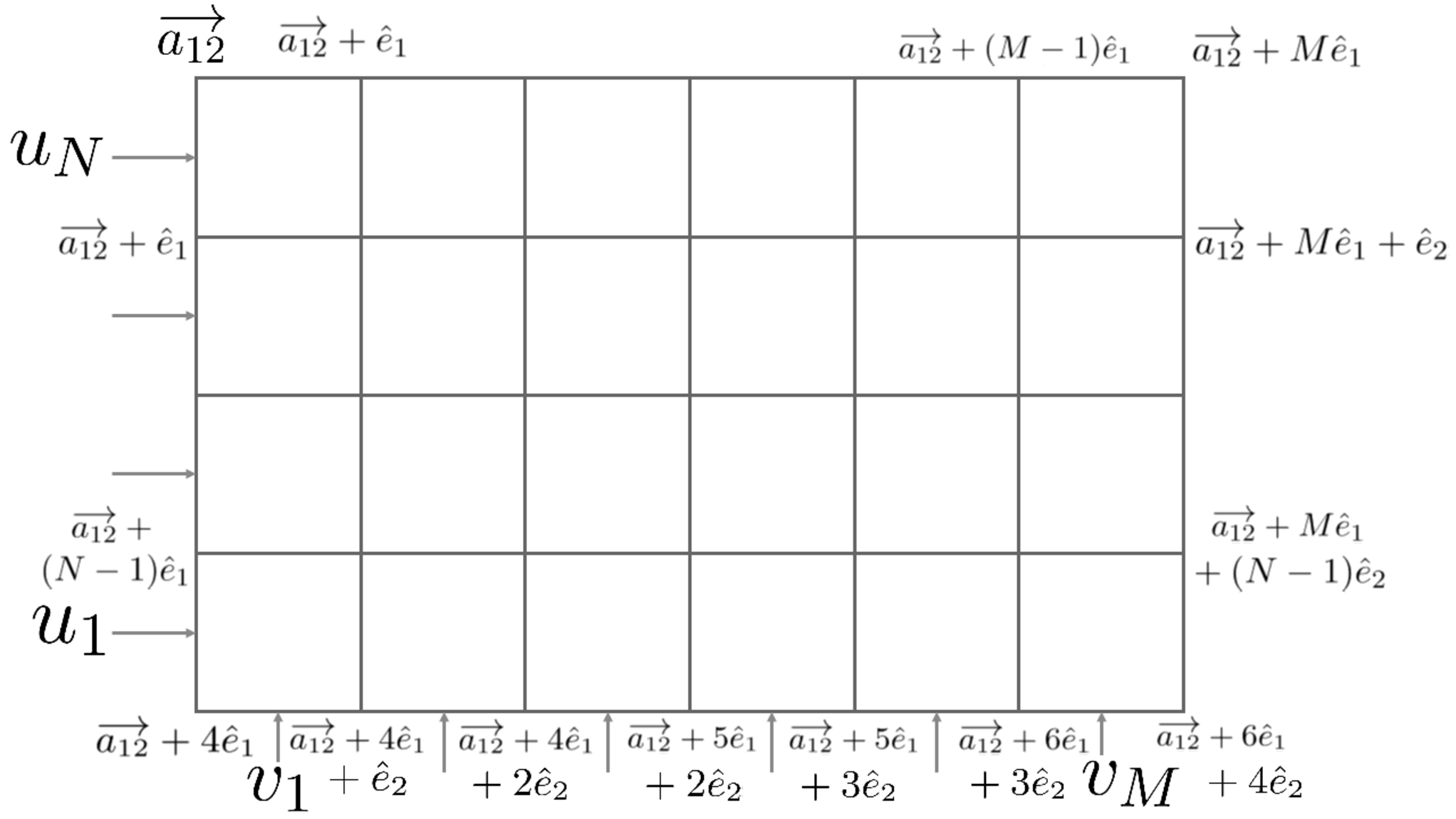
Figure 5: The partition functions WM,N(u1,…,uN|v1,…,vM|x1,…,xN|a12)W_{M,N}(u_{1},\dots,u_{N}|v_{1},\dots,v_{M}|x_{1},\dots,x_{N}|a_{12}) (2.2).
Refer to caption
Figure 6: An example W6,4(u1,…,u4|v1,…,v6|1,2,4,6|a12)W_{6,4}(u_{1},\dots,u_{4}|v_{1},\dots,v_{6}|1,2,4,6|a_{12}) of the partition functions (2.2). Note that x1=1x_{1}=1, x2=2x_{2}=2, x3=4x_{3}=4, x4=6x_{4}=6 labels the positions of the edges of the bottom part of the partition functions where the difference of the adjacent state vectors of the vertices is e^2\hat{e}_{2}.
Refer to caption
Figure 7: A graphical description of a summand in the decompostion of the partition functions (3.5). The unshaded part and the shaded part corresponds to Pj(u1,…,uN|v1,…,vM−1|x1,…,xN−1|a12)P_{j}(u_{1},\dots,u_{N}|v_{1},\dots,v_{M-1}|x_{1},\dots,x_{N-1}|a_{12}) (3) and W~j​(u1,…,uN​|vM|​a12)\widetilde{W}_{j}(u_{1},\dots,u_{N}|v_{M}|a_{12}) (3) , respectively.
Refer to caption
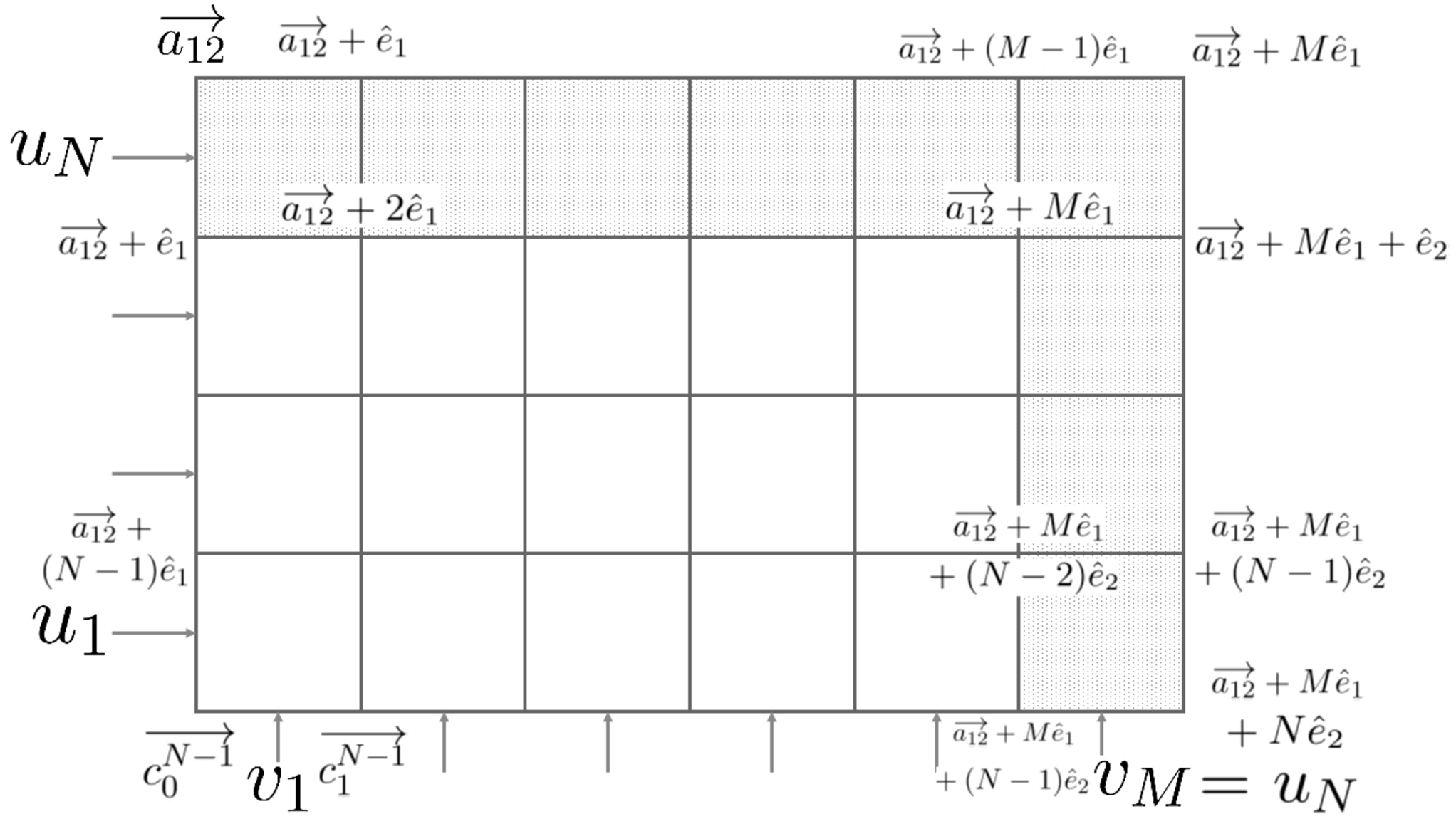
Figure 8: The recursion relation WM,N(u1,…,uN|v1,…,vM|x1,…,xN|a12)W_{M,N}(u_{1},\dots,u_{N}|v_{1},\dots,v_{M}|x_{1},\dots,x_{N}|a_{12}), xN=Mx_{N}=M evaluated at vM=uNv_{M}=u_{N} (3.2) . The states of the vertices around the shaded faces are freezed.
Refer to caption
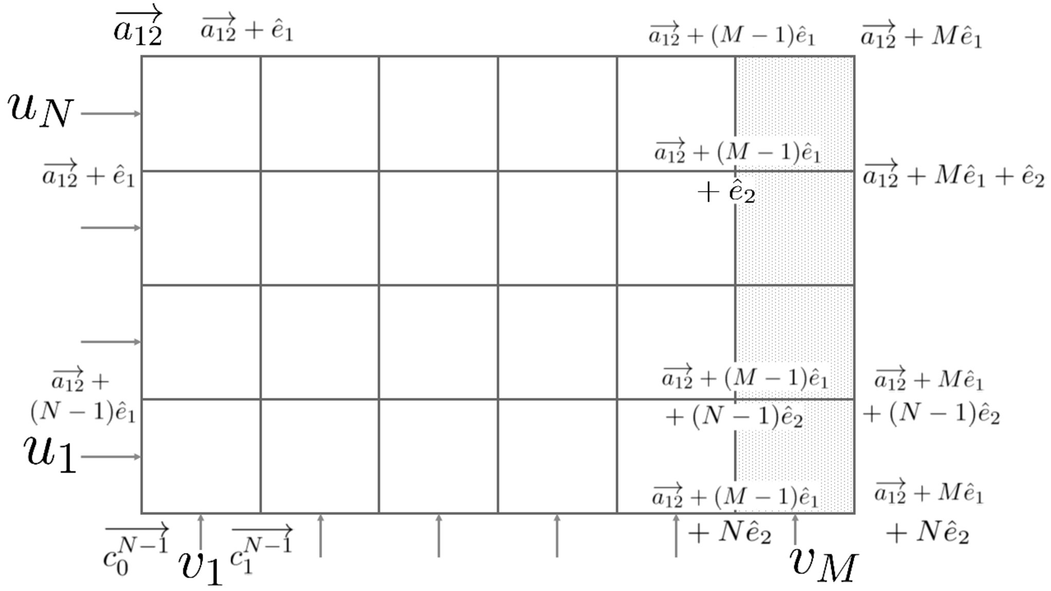
Figure 9: The factorization of WM,N(u1,…,uN|v1,…,vM|x1,…,xN|a12)W_{M,N}(u_{1},\dots,u_{N}|v_{1},\dots,v_{M}|x_{1},\dots,x_{N}|a_{12}), xN≠Mx_{N}\neq M (3.3) . The states of the vertices around the shaded faces are freezed.

See Figures 5 and 6 for pictorial descriptions of the definition and an example of the partition functions (2.2). In the next section, we examine the properties of the partition functions.

3 Izergin-Korepin analysis

In this section, we determine the properties of the partition functions of the elliptic supersymmetric face model WM,N(u1,…,uN|v1,…,vM|x1,…,xN|a12)W_{M,N}(u_{1},\dots,u_{N}|v_{1},\dots,v_{M}|x_{1},\dots,x_{N}|a_{12}) by extending the Izergin-Korepin analysis on the domain wall boundary partition functions [39, 40].

Proposition 3.1.

The partition functions WM,N(u1,…,uN|v1,…,vM|x1,…,xN|a12)W_{M,N}(u_{1},\dots,u_{N}|v_{1},\dots,v_{M}|x_{1},\dots,x_{N}|a_{12}) satisfies the following properties.

(1) When xN=Mx_{N}=M, the partition functions WM,N(u1,…,uN|v1,…,vM|x1,…,xN|a12)W_{M,N}(u_{1},\dots,u_{N}|v_{1},\dots,v_{M}|x_{1},\dots,x_{N}|a_{12}), regarded as a polynomial in yM:=λ2​K1​vM\displaystyle y_{M}:=\frac{\lambda}{2K_{1}}v_{M}, is an elliptic polynomial in ΘN​(χ)\Theta_{N}(\chi).
(2) The partition functions WM,N(uσ⁡(1),…,uσ⁡(N)|v1,…,vM|x1,…,xN|a12)W_{M,N}(u_{\sigma(1)},\dots,u_{\sigma(N)}|v_{1},\dots,v_{M}|x_{1},\dots,x_{N}|a_{12}) with the ordering of the spectral parameters permuted uσ⁡(1),…,uσ⁡(N)u_{\sigma(1)},\dots,u_{\sigma(N)}, σ∈SN\sigma\in S_{N} are related with the unpermuted one WM,N(u1,…,uN|v1,…,vM|x1,…,xN|a12)W_{M,N}(u_{1},\dots,u_{N}|v_{1},\dots,v_{M}|x_{1},\dots,x_{N}|a_{12}) by the following relation

∏1≤j<k≤Nσ⁡(j)>σ⁡(k)[1+uσ⁡(k)−uσ⁡(j)]WM,N(u1,…,uN|v1,…,vM|x1,…,xN|a12)\displaystyle\prod_{\begin{subarray}{c}1\leq j<k\leq N\\ \sigma(j)>\sigma(k)\end{subarray}}[1+u_{\sigma(k)}-u_{\sigma(j)}]W_{M,N}(u_{1},\dots,u_{N}|v_{1},\dots,v_{M}|x_{1},\dots,x_{N}|a_{12})
=\displaystyle= ∏1≤j<k≤Nσ⁡(j)>σ⁡(k)[1+uσ⁡(j)−uσ⁡(k)]WM,N(uσ⁡(1),…,uσ⁡(N)|v1,…,vM|x1,…,xN|a12).\displaystyle\prod_{\begin{subarray}{c}1\leq j<k\leq N\\ \sigma(j)>\sigma(k)\end{subarray}}[1+u_{\sigma(j)}-u_{\sigma(k)}]W_{M,N}(u_{\sigma(1)},\dots,u_{\sigma(N)}|v_{1},\dots,v_{M}|x_{1},\dots,x_{N}|a_{12}). (3.1)

(3) The following recursive relations between the partition functions hold if xN=Mx_{N}=M (Figure 8):

WM,N(u1,…,uN|v1,…,vM|x1,…,xN|a12)|vM=uN\displaystyle W_{M,N}(u_{1},\dots,u_{N}|v_{1},\dots,v_{M}|x_{1},\dots,x_{N}|a_{12})|_{v_{M}=u_{N}}
=\displaystyle= ∏j=1N−1[1−uj+uN][1]​∏j=1M−1[1+uN−vj][1]\displaystyle\prod_{j=1}^{N-1}\frac{[1-u_{j}+u_{N}]}{[1]}\prod_{j=1}^{M-1}\frac{[1+u_{N}-v_{j}]}{[1]}
×WM−1,N−1(u1,…,uN−1|v1,…,vM−1|x1,…,xN−1|a12+1).\displaystyle\times W_{M-1,N-1}(u_{1},\dots,u_{N-1}|v_{1},\dots,v_{M-1}|x_{1},\dots,x_{N-1}|a_{12}+1). (3.2)

If xN≠Mx_{N}\neq M, the following factorizations hold for the partition functions (Figure 9):

WM,N(u1,…,uN|v1,…,vM|x1,…,xN|a12)\displaystyle W_{M,N}(u_{1},\dots,u_{N}|v_{1},\dots,v_{M}|x_{1},\dots,x_{N}|a_{12})
=\displaystyle= [a21−M−N+1][a21−M+1]∏j=1N[uj−vM][1]WM−1,N(u1,…,uN|v1,…,vM−1|x1,…,xN|a12).\displaystyle\frac{[a_{21}-M-N+1]}{[a_{21}-M+1]}\prod_{j=1}^{N}\frac{[u_{j}-v_{M}]}{[1]}W_{M-1,N}(u_{1},\dots,u_{N}|v_{1},\dots,v_{M-1}|x_{1},\dots,x_{N}|a_{12}). (3.3)

(4) The following holds for the case N=1N=1, x1=Mx_{1}=M

WM,1​(u|v1,…,vM​|M|​a12)=[−u+vM+a12+M−1][a12+M−1]​∏k=1M−1[1+u−vk][1].\displaystyle W_{M,1}(u|v_{1},\dots,v_{M}|M|a_{12})=\frac{[-u+v_{M}+a_{12}+M-1]}{[a_{12}+M-1]}\prod_{k=1}^{M-1}\frac{[1+u-v_{k}]}{[1]}. (3.4)
Proof.

Properties (1), (2) and (3) for the case xN=Mx_{N}=M can be proved essentially in the same way with the domain wall boundary partition functions, which is given in the PhD thesis of Zuparic [46] (note there is a small difference in the setting. For example, the ordering of the spectral parameters is inverted). We just have to treat the case xN≠Mx_{N}\neq M separately, which is given as the factorization formula of the partition functions in Property (3).

To show Property (1), we first decompose the partition functions satisfying xN=Mx_{N}=M in the following form as we do for the case of vertex models. We split the partition functions as a sum of the products of the partition functions Pj(u1,…,uN|v1,…,vM−1|x1,…,xN−1|a12)P_{j}(u_{1},\dots,u_{N}|v_{1},\dots,v_{M-1}|x_{1},\dots,x_{N-1}|a_{12}) and one-column partition functions W~j​(u1,…,uN​|vM|​a12)\widetilde{W}_{j}(u_{1},\dots,u_{N}|v_{M}|a_{12}) (see Figure 7 for this decomposition)

WM,N(u1,…,uN|v1,…,vM|x1,…,xN|a12)\displaystyle W_{M,N}(u_{1},\dots,u_{N}|v_{1},\dots,v_{M}|x_{1},\dots,x_{N}|a_{12})
=\displaystyle= ∑j=0N−1Pj(u1,…,uN|v1,…,vM−1|x1,…,xN−1|a12)W~j(u1,…,uN|vM|a12).\displaystyle\sum_{j=0}^{N-1}P_{j}(u_{1},\dots,u_{N}|v_{1},\dots,v_{M-1}|x_{1},\dots,x_{N-1}|a_{12})\widetilde{W}_{j}(u_{1},\dots,u_{N}|v_{M}|a_{12}). (3.5)

Here, W~j​(u1,…,uN​|vM|​a12)\widetilde{W}_{j}(u_{1},\dots,u_{N}|v_{M}|a_{12}) are the one-column partition functions corresponding to the shaded part in Figure 7

W~j​(u1,…,uN​|vM|​a12)\displaystyle\widetilde{W}_{j}(u_{1},\dots,u_{N}|v_{M}|a_{12})
=\displaystyle= ∏k=0j−1W⁡(a12→+(M−1)​e^1+k​e^2a12→+M​e^1+k​e^2a12→+(M−1)​e^1+(k+1)​e^2a12→+M​e^1+(k+1)​e^2​|uN−k|​vM)\displaystyle\prod_{k=0}^{j-1}W\Bigg(\begin{array}[]{cc}\overrightarrow{a_{12}}+(M-1)\hat{e}_{1}+k\hat{e}_{2}&\overrightarrow{a_{12}}+M\hat{e}_{1}+k\hat{e}_{2}\\ \overrightarrow{a_{12}}+(M-1)\hat{e}_{1}+(k+1)\hat{e}_{2}&\overrightarrow{a_{12}}+M\hat{e}_{1}+(k+1)\hat{e}_{2}\end{array}\Bigg|u_{N-k}\Bigg|v_{M}\Bigg)
×W⁡(a12→+(M−1)​e^1+j​e^2a12→+M​e^1+j​e^2a12→+M​e^1+j​e^2a12→+M​e^1+(j+1)​e^2​|uN−j|​vM)\displaystyle\times W\Bigg(\begin{array}[]{cc}\overrightarrow{a_{12}}+(M-1)\hat{e}_{1}+j\hat{e}_{2}&\overrightarrow{a_{12}}+M\hat{e}_{1}+j\hat{e}_{2}\\ \overrightarrow{a_{12}}+M\hat{e}_{1}+j\hat{e}_{2}&\overrightarrow{a_{12}}+M\hat{e}_{1}+(j+1)\hat{e}_{2}\end{array}\Bigg|u_{N-j}\Bigg|v_{M}\Bigg)
×∏k=jN−2W⁡(a12→+M​e^1+k​e^2a12→+M​e^1+(k+1)​e^2a12→+M​e^1+(k+1)​e^2a12→+M​e^1+(k+2)​e^2​|uN−k−1|​vM).\displaystyle\times\prod_{k=j}^{N-2}W\Bigg(\begin{array}[]{cc}\overrightarrow{a_{12}}+M\hat{e}_{1}+k\hat{e}_{2}&\overrightarrow{a_{12}}+M\hat{e}_{1}+(k+1)\hat{e}_{2}\\ \overrightarrow{a_{12}}+M\hat{e}_{1}+(k+1)\hat{e}_{2}&\overrightarrow{a_{12}}+M\hat{e}_{1}+(k+2)\hat{e}_{2}\end{array}\Bigg|u_{N-k-1}\Bigg|v_{M}\Bigg).

The partition functions Pj(u1,…,uN|v1,…,vM−1|x1,…,xN−1|a12)P_{j}(u_{1},\dots,u_{N}|v_{1},\dots,v_{M-1}|x_{1},\dots,x_{N-1}|a_{12}) corresponding to the unshaded part in Figure 7 is explicitly written as

Pj(u1,…,uN|v1,…,vM−1|x1,…,xN−1|a12)=∑{b0→},{b1→},…,{bN−2→}\displaystyle P_{j}(u_{1},\dots,u_{N}|v_{1},\dots,v_{M-1}|x_{1},\dots,x_{N-1}|a_{12})=\sum_{\{\overrightarrow{b^{0}}\},\{\overrightarrow{b^{1}}\},\dots,\{\overrightarrow{b^{N-2}}\}}
TM−10​(a12→a12→+e^1⋯a12→+(M−2)​e^1a12→+(M−1)​e^1a12→+e^1b10→⋯bM−20→a12→+(M−1)​e^1+e^2|uN)\displaystyle T_{M-1}^{0}\Bigg(\begin{array}[]{ccccc}\overrightarrow{a_{12}}&\overrightarrow{a_{12}}+\hat{e}_{1}&\cdots&\overrightarrow{a_{12}}+(M-2)\hat{e}_{1}&\overrightarrow{a_{12}}+(M-1)\hat{e}_{1}\\ \overrightarrow{a_{12}}+\hat{e}_{1}&\overrightarrow{b_{1}^{0}}&\cdots&\overrightarrow{b_{M-2}^{0}}&\overrightarrow{a_{12}}+(M-1)\hat{e}_{1}+\hat{e}_{2}\end{array}\Bigg|u_{N}\Bigg)
×∏k=1j−1\displaystyle\times\prod_{k=1}^{j-1} TM−1k​(a12→+k​e^1b1k−1→⋯bM−2k−1→a12→+(M−1)​e^1+k​e^2a12→+(k+1)​e^1b1k→⋯bM−2k→a12→+(M−1)​e^1+(k+1)​e^2|uN−k)\displaystyle T_{M-1}^{k}\Bigg(\begin{array}[]{ccccc}\overrightarrow{a_{12}}+k\hat{e}_{1}&\overrightarrow{b_{1}^{k-1}}&\cdots&\overrightarrow{b_{M-2}^{k-1}}&\overrightarrow{a_{12}}+(M-1)\hat{e}_{1}+k\hat{e}_{2}\\ \overrightarrow{a_{12}}+(k+1)\hat{e}_{1}&\overrightarrow{b_{1}^{k}}&\cdots&\overrightarrow{b_{M-2}^{k}}&\overrightarrow{a_{12}}+(M-1)\hat{e}_{1}+(k+1)\hat{e}_{2}\end{array}\Bigg|u_{N-k}\Bigg)
×\displaystyle\times TM−1j​(a12→+j​e^1b1j−1→⋯bM−2j−1→a12→+(M−1)​e^1+j​e^2a12→+(j+1)​e^1b1j→⋯bM−2j→a12→+M​e^1+j​e^2|uN−j)\displaystyle T_{M-1}^{j}\Bigg(\begin{array}[]{ccccc}\overrightarrow{a_{12}}+j\hat{e}_{1}&\overrightarrow{b_{1}^{j-1}}&\cdots&\overrightarrow{b_{M-2}^{j-1}}&\overrightarrow{a_{12}}+(M-1)\hat{e}_{1}+j\hat{e}_{2}\\ \overrightarrow{a_{12}}+(j+1)\hat{e}_{1}&\overrightarrow{b_{1}^{j}}&\cdots&\overrightarrow{b_{M-2}^{j}}&\overrightarrow{a_{12}}+M\hat{e}_{1}+j\hat{e}_{2}\end{array}\Bigg|u_{N-j}\Bigg)
×∏k=j+1N−2\displaystyle\times\prod_{k=j+1}^{N-2} TM−1k​(a12→+k​e^1b1k−1→⋯bM−2k−1→a12→+M​e^1+(k−1)​e^2a12→+(k+1)​e^1b1k→⋯bM−2k→a12→+M​e^1+k​e^2|uN−k)\displaystyle T_{M-1}^{k}\Bigg(\begin{array}[]{ccccc}\overrightarrow{a_{12}}+k\hat{e}_{1}&\overrightarrow{b_{1}^{k-1}}&\cdots&\overrightarrow{b_{M-2}^{k-1}}&\overrightarrow{a_{12}}+M\hat{e}_{1}+(k-1)\hat{e}_{2}\\ \overrightarrow{a_{12}}+(k+1)\hat{e}_{1}&\overrightarrow{b_{1}^{k}}&\cdots&\overrightarrow{b_{M-2}^{k}}&\overrightarrow{a_{12}}+M\hat{e}_{1}+k\hat{e}_{2}\end{array}\Bigg|u_{N-k}\Bigg)
×\displaystyle\times TM−1N−1​(a12→+(N−1)​e^1b1N−2→⋯bM−2N−2→a12→+M​e^1+(N−2)​e^2d0N−1→d1N−1→⋯dM−2N−1→dM−1N−1→|u1),\displaystyle T_{M-1}^{N-1}\Bigg(\begin{array}[]{ccccc}\overrightarrow{a_{12}}+(N-1)\hat{e}_{1}&\overrightarrow{b_{1}^{N-2}}&\cdots&\overrightarrow{b_{M-2}^{N-2}}&\overrightarrow{a_{12}}+M\hat{e}_{1}+(N-2)\hat{e}_{2}\\ \overrightarrow{d_{0}^{N-1}}&\overrightarrow{d_{1}^{N-1}}&\cdots&\overrightarrow{d_{M-2}^{N-1}}&\overrightarrow{d_{M-1}^{N-1}}\end{array}\Bigg|u_{1}\Bigg),

where the state vectors d0N−1→,d1N−1→,…,dM−2N−1→,dM−1N−1→\overrightarrow{d_{0}^{N-1}},\overrightarrow{d_{1}^{N-1}},\dots,\overrightarrow{d_{M-2}^{N-1}},\overrightarrow{d_{M-1}^{N-1}} are fixed using the sequence of integers 1≤x1<x2<⋯<xN−1≤M−11\leq x_{1}<x_{2}<\cdots<x_{N-1}\leq M-1 as

d0N−1→,d1N−1→,…,dM−2N−1→,dM−1N−1→\displaystyle\overrightarrow{d_{0}^{N-1}},\overrightarrow{d_{1}^{N-1}},\dots,\overrightarrow{d_{M-2}^{N-1}},\overrightarrow{d_{M-1}^{N-1}}
=\displaystyle= a12→+N​e^1,…,a12→+(N+x1−1)​e^1,a12→+(N+x1−1)​e^1+e^2,\displaystyle\overrightarrow{a_{12}}+N\hat{e}_{1},\dots,\overrightarrow{a_{12}}+(N+x_{1}-1)\hat{e}_{1},\overrightarrow{a_{12}}+(N+x_{1}-1)\hat{e}_{1}+\hat{e}_{2},
a12→+(N+x1)​e^1+e^2,…,a12→+(N+x1+x2−3)​e^1+e^2,a12→+(N+x1+x2−3)​e^1+2​e^2,\displaystyle\overrightarrow{a_{12}}+(N+x_{1})\hat{e}_{1}+\hat{e}_{2},\dots,\overrightarrow{a_{12}}+(N+x_{1}+x_{2}-3)\hat{e}_{1}+\hat{e}_{2},\overrightarrow{a_{12}}+(N+x_{1}+x_{2}-3)\hat{e}_{1}+2\hat{e}_{2},
a12→+(N+x1+x2−2)​e^1+2​e^2,…,a12→+M​e^1+(N−1)​e^2.\displaystyle\overrightarrow{a_{12}}+(N+x_{1}+x_{2}-2)\hat{e}_{1}+2\hat{e}_{2},\dots,\overrightarrow{a_{12}}+M\hat{e}_{1}+(N-1)\hat{e}_{2}. (3.22)

We have omitted writing the dependence on the inhomogeneous parameters in TM−1kT_{M-1}^{k} in (3). It depends on v1,…,vM−1v_{1},\dots,v_{M-1}, but not on vMv_{M}. This means that (3) does not depend on the inhomogeneous parameter vMv_{M}, so we only have to examine the other parts (3) if one analyzes the partition functions as a function of vMv_{M}. From the definition of the weights (2.2), (2.2), (2.2), W~j​(u1,…,uN​|vM|​a12)\widetilde{W}_{j}(u_{1},\dots,u_{N}|v_{M}|a_{12}) is explicitly calculated as

W~j​(u1,…,uN​|vM|​a12)=[a12+M−1+j−uN−j+vM][a12+M−1+j]\displaystyle\widetilde{W}_{j}(u_{1},\dots,u_{N}|v_{M}|a_{12})=\frac{[a_{12}+M-1+j-u_{N-j}+v_{M}]}{[a_{12}+M-1+j]}
×\displaystyle\times ∏k=N−j+1N[uk−vM]​[a21−M+k−N][1]​[a21−M+1+k−N]​∏k=1N−j−1[1−uk+vM][1].\displaystyle\prod_{k=N-j+1}^{N}\frac{[u_{k}-v_{M}][a_{21}-M+k-N]}{[1][a_{21}-M+1+k-N]}\prod_{k=1}^{N-j-1}\frac{[1-u_{k}+v_{M}]}{[1]}. (3.23)

We then view W~j​(u1,…,uN​|vM|​a12)\widetilde{W}_{j}(u_{1},\dots,u_{N}|v_{M}|a_{12}) as a function of vMv_{M}. From its explicit form (3.23) and using (2.11) and (2.12), a12=−a21a_{12}=-a_{21} and [−u]=−[u][-u]=-[u], one easily calculates the quasi-periodicities of the function W~j​(u1,…,uN​|vM|​a12)\widetilde{W}_{j}(u_{1},\dots,u_{N}|v_{M}|a_{12})

W~j​(u1,…,uN​|vM+2​K1/λ|​a12)\displaystyle\widetilde{W}_{j}(u_{1},\dots,u_{N}|v_{M}+2K_{1}/\lambda|a_{12})
=\displaystyle= (−1)N​W~j​(u1,…,uN​|vM|​a12),\displaystyle(-1)^{N}\widetilde{W}_{j}(u_{1},\dots,u_{N}|v_{M}|a_{12}), (3.24)
W~j​(u1,…,uN​|vM+2​i​K2/λ|​a12)\displaystyle\widetilde{W}_{j}(u_{1},\dots,u_{N}|v_{M}+2iK_{2}/\lambda|a_{12})
=\displaystyle= (−q−1)N​exp​(−i​π​λK1​(N​vM−∑j=1Nuj+a12+N+M−2))​W~j​(u1,…,uN​|vM|​a12).\displaystyle(-q^{-1})^{N}\mathrm{exp}\Bigg(-\frac{i\pi\lambda}{K_{1}}\Bigg(Nv_{M}-\sum_{j=1}^{N}u_{j}+a_{12}+N+M-2\Bigg)\Bigg)\widetilde{W}_{j}(u_{1},\dots,u_{N}|v_{M}|a_{12}). (3.25)

From (3.24), (3.25) and (3.5), one finds the same quasi-periodicities as above also hold for the partition functions

WM,N(u1,…,uN|v1,…,vM+2K1/λ|x1,…,xN|a12)\displaystyle W_{M,N}(u_{1},\dots,u_{N}|v_{1},\dots,v_{M}+2K_{1}/\lambda|x_{1},\dots,x_{N}|a_{12})
=\displaystyle= (−1)NWM,N(u1,…,uN|v1,…,vM|x1,…,xN|a12),\displaystyle(-1)^{N}W_{M,N}(u_{1},\dots,u_{N}|v_{1},\dots,v_{M}|x_{1},\dots,x_{N}|a_{12}), (3.26)
WM,N(u1,…,uN|v1,…,vM+2iK2/λ|x1,…,xN|a12)\displaystyle W_{M,N}(u_{1},\dots,u_{N}|v_{1},\dots,v_{M}+2iK_{2}/\lambda|x_{1},\dots,x_{N}|a_{12})
=\displaystyle= (−q−1)N​exp​(−i​π​λK1​(N​vM−∑j=1Nuj+a12+N+M−2))\displaystyle(-q^{-1})^{N}\mathrm{exp}\Bigg(-\frac{i\pi\lambda}{K_{1}}\Bigg(Nv_{M}-\sum_{j=1}^{N}u_{j}+a_{12}+N+M-2\Bigg)\Bigg)
×WM,N(u1,…,uN|v1,…,vM|x1,…,xN|a12).\displaystyle\times W_{M,N}(u_{1},\dots,u_{N}|v_{1},\dots,v_{M}|x_{1},\dots,x_{N}|a_{12}). (3.27)

If we rescale the parameter from vMv_{M} to yM:=λ2​K1​vM\displaystyle y_{M}:=\frac{\lambda}{2K_{1}}v_{M}, and define ϕ⁡(yM)\phi(y_{M}) as

ϕ(yM)=WM,N(u1,…,uN|v1,…,vM|x1,…,xN|a12),\displaystyle\phi(y_{M})=W_{M,N}(u_{1},\dots,u_{N}|v_{1},\dots,v_{M}|x_{1},\dots,x_{N}|a_{12}), (3.28)

the quasi-periodicities (3.26) and (3.27) for WM,N(u1,…,uN|v1,…,vM|x1,…,xN|a12)W_{M,N}(u_{1},\dots,u_{N}|v_{1},\dots,v_{M}|x_{1},\dots,x_{N}|a_{12}) can be rewritten as a function ϕ⁡(yM)\phi(y_{M}) of yMy_{M} as

ϕ⁡(yM+1)\displaystyle\phi(y_{M}+1) =(−1)N​ϕ​(yM),\displaystyle=(-1)^{N}\phi(y_{M}), (3.29)
ϕ⁡(yM+τ)\displaystyle\phi(y_{M}+\tau) =(−1)N​exp​(π​λ​τK2​(∑j=1Nuj−a12−N−M+2))​e−2​π​i​N​yM−π​i​N​τ​ϕ​(yM),\displaystyle=(-1)^{N}\mathrm{exp}\Bigg(\frac{\pi\lambda\tau}{K_{2}}\Bigg(\sum_{j=1}^{N}u_{j}-a_{12}-N-M+2\Bigg)\Bigg)e^{-2\pi iNy_{M}-\pi iN\tau}\phi(y_{M}), (3.30)

where the nome τ\tau is given by τ=i​K2K1\displaystyle\tau=i\frac{K_{2}}{K_{1}}. These are exactly the quasi-periodicities (2.6), (2.7) with characters χ⁡(1)=(−1)N\chi(1)=(-1)^{N}, χ⁡(τ)=(−1)N​exp​(π​λ​τK2​(∑j=1Nuj−a12−N−M+2))\displaystyle\chi(\tau)=(-1)^{N}\mathrm{exp}\Bigg(\frac{\pi\lambda\tau}{K_{2}}\Bigg(\sum_{j=1}^{N}u_{j}-a_{12}-N-M+2\Bigg)\Bigg). Hence, it is an elliptic polynomial in ΘN​(χ)\Theta_{N}(\chi).

Property (2) can also be shown in a standard way. By attaching a face having the weight
W⁡(a12→+M​e^1+(N−j−1)​e^2a12→+M​e^1+(N−j)​e^2a12→+M​e^1+(N−j)​e^2a12→+M​e^1+(N−j+1)​e^2​|uj+1|​uj)W\Bigg(\begin{array}[]{cc}\overrightarrow{a_{12}}+M\hat{e}_{1}+(N-j-1)\hat{e}_{2}&\overrightarrow{a_{12}}+M\hat{e}_{1}+(N-j)\hat{e}_{2}\\ \overrightarrow{a_{12}}+M\hat{e}_{1}+(N-j)\hat{e}_{2}&\overrightarrow{a_{12}}+M\hat{e}_{1}+(N-j+1)\hat{e}_{2}\end{array}\Bigg|u_{j+1}\Bigg|u_{j}\Bigg) on the right side of the partition functions WM,N(u1,…,uN|v1,…,vM|x1,…,xN|a12)W_{M,N}(u_{1},\dots,u_{N}|v_{1},\dots,v_{M}|x_{1},\dots,x_{N}|a_{12}) and using the face-type Yang-Baxter relation (2.2) repeatedly, a face having the weight
W⁡(a12→+(N−j−1)​e^1a12→+(N−j)​e^1a12→+(N−j)​e^1a12→+(N−j+1)​e^1​|uj+1|​uj)W\Bigg(\begin{array}[]{cc}\overrightarrow{a_{12}}+(N-j-1)\hat{e}_{1}&\overrightarrow{a_{12}}+(N-j)\hat{e}_{1}\\ \overrightarrow{a_{12}}+(N-j)\hat{e}_{1}&\overrightarrow{a_{12}}+(N-j+1)\hat{e}_{1}\end{array}\Bigg|u_{j+1}\Bigg|u_{j}\Bigg) gets out of the left side of the partition functions. The ordering of the spectral parameters of the partition functions is now changed to WM,N(u1,…,uj+1,uj,…,uN|v1,…,vM|x1,…,xN|a12)W_{M,N}(u_{1},\dots,u_{j+1},u_{j},\dots,u_{N}|v_{1},\dots,v_{M}|x_{1},\dots,x_{N}|a_{12}), and we get

W⁡(a12→+M​e^1+(N−j−1)​e^2a12→+M​e^1+(N−j)​e^2a12→+M​e^1+(N−j)​e^2a12→+M​e^1+(N−j+1)​e^2​|uj+1|​uj)\displaystyle W\Bigg(\begin{array}[]{cc}\overrightarrow{a_{12}}+M\hat{e}_{1}+(N-j-1)\hat{e}_{2}&\overrightarrow{a_{12}}+M\hat{e}_{1}+(N-j)\hat{e}_{2}\\ \overrightarrow{a_{12}}+M\hat{e}_{1}+(N-j)\hat{e}_{2}&\overrightarrow{a_{12}}+M\hat{e}_{1}+(N-j+1)\hat{e}_{2}\end{array}\Bigg|u_{j+1}\Bigg|u_{j}\Bigg)
×\displaystyle\times WM,N(u1,…,uN|v1,…,vM|x1,…,xN|a12)\displaystyle W_{M,N}(u_{1},\dots,u_{N}|v_{1},\dots,v_{M}|x_{1},\dots,x_{N}|a_{12})
=\displaystyle= W⁡(a12→+(N−j−1)​e^1a12→+(N−j)​e^1a12→+(N−j)​e^1a12→+(N−j+1)​e^1​|uj+1|​uj)\displaystyle W\Bigg(\begin{array}[]{cc}\overrightarrow{a_{12}}+(N-j-1)\hat{e}_{1}&\overrightarrow{a_{12}}+(N-j)\hat{e}_{1}\\ \overrightarrow{a_{12}}+(N-j)\hat{e}_{1}&\overrightarrow{a_{12}}+(N-j+1)\hat{e}_{1}\end{array}\Bigg|u_{j+1}\Bigg|u_{j}\Bigg)
×\displaystyle\times WM,N(u1,…,uj+1,uj,…,uN|v1,…,vM|x1,…,xN|a12).\displaystyle W_{M,N}(u_{1},\dots,u_{j+1},u_{j},\dots,u_{N}|v_{1},\dots,v_{M}|x_{1},\dots,x_{N}|a_{12}). (3.35)

Simplifying the above equality, we have

[1+uj−uj+1]WM,N(u1,…,uN|v1,…,vM|x1,…,xN|a12)\displaystyle[1+u_{j}-u_{j+1}]W_{M,N}(u_{1},\dots,u_{N}|v_{1},\dots,v_{M}|x_{1},\dots,x_{N}|a_{12})
=\displaystyle= [1+uj+1−uj]WM,N(u1,…,uj+1,uj,…,uN|v1,…,vM|x1,…,xN|a12).\displaystyle[1+u_{j+1}-u_{j}]W_{M,N}(u_{1},\dots,u_{j+1},u_{j},\dots,u_{N}|v_{1},\dots,v_{M}|x_{1},\dots,x_{N}|a_{12}). (3.36)

The general case (3.1) can be obtained by using the commutation relation (3.36) repeatedly. For example, the case N=3N=3, σ=(3,1,2)\sigma=(3,1,2) can be shown as follows:

WM,3(u1,u2,u3|v1,…,vM|x1,x2,x3|a12)\displaystyle W_{M,3}(u_{1},u_{2},u_{3}|v_{1},\dots,v_{M}|x_{1},x_{2},x_{3}|a_{12})
=\displaystyle= [1+u3−u2][1+u2−u3]WM,3(u1,u3,u2|v1,…,vM|x1,x2,x3|a12)\displaystyle\frac{[1+u_{3}-u_{2}]}{[1+u_{2}-u_{3}]}W_{M,3}(u_{1},u_{3},u_{2}|v_{1},\dots,v_{M}|x_{1},x_{2},x_{3}|a_{12})
=\displaystyle= [1+u3−u2][1+u2−u3][1+u3−u1][1+u1−u3]WM,3(u3,u1,u2|v1,…,vM|x1,x2,x3|a12).\displaystyle\frac{[1+u_{3}-u_{2}]}{[1+u_{2}-u_{3}]}\frac{[1+u_{3}-u_{1}]}{[1+u_{1}-u_{3}]}W_{M,3}(u_{3},u_{1},u_{2}|v_{1},\dots,v_{M}|x_{1},x_{2},x_{3}|a_{12}). (3.37)

Let us show Property (3) for the case xN=Mx_{N}=M. Before showing this, we remark that from Property (1), the partition functions WM,N(u1,…,uN|v1,…,vM|x1,…,xN|a12)W_{M,N}(u_{1},\dots,u_{N}|v_{1},\dots,v_{M}|x_{1},\dots,x_{N}|a_{12}) is an elliptic polynomial of degree NN in vMv_{M}, and the properties of the elliptic polynomials listed in Proposition 2.1 allow us to use the Izergin-Korepin trick. If one relates the evaluations of the partition functions at NN distinct points in vMv_{M} with smaller ones, and if one can find the functions satisfying the same recursion, then the Izergin-Korepin method is successful. One should keep in mind that for the case of the partition functions, one has another case xN≠Mx_{N}\neq M, which must be taken into account. We also need Property (4) to assure the uniqueness, since this property corresponds to the initial condition of the recursion relation. (3.2) is the result of the evaluation of the partition functions at the point vM=uNv_{M}=u_{N}. The other (N−1)(N-1) points vM=ujv_{M}=u_{j}, j=1,…,N−1j=1,\dots,N-1 can be evaluated using Property (2), hence if one shows that certain explicit functions satisfy Property (2) and the evaluation at vM=uNv_{M}=u_{N}, the proof of the recursion relation for the case xN=Mx_{N}=M is succeeded. This will be performed in section 5.

One can show the recursion relation (3.2) by using the graphical representation of the partition functions WM,N(u1,…,uN|v1,…,vM|x1,…,xN|a12)W_{M,N}(u_{1},\dots,u_{N}|v_{1},\dots,v_{M}|x_{1},\dots,x_{N}|a_{12}) (see Figure 8). If one sets vM=uNv_{M}=u_{N} and use W⁡(a→a→+e^1a→+e^2a→+e^1+e^2​|uN|​vM)|vM=uN=0W\Bigg(\begin{array}[]{cc}\overrightarrow{a}&\overrightarrow{a}+\hat{e}_{1}\\ \overrightarrow{a}+\hat{e}_{2}&\overrightarrow{a}+\hat{e}_{1}+\hat{e}_{2}\end{array}\Bigg|u_{N}\Bigg|v_{M}\Bigg)\Bigg|_{v_{M}=u_{N}}=0, one first finds that the state vectors around the face of the top right corner freeze. Continuing graphical considerations, one finds that all the state vectors at the rightmost column and the top row freeze. One can also see that the state of the top left corner of remaining unfreezed part is now a12→+e^1\overrightarrow{a_{12}}+\hat{e}_{1}, thus the unfreezed part is the partition functions WM−1,N−1(u1,…,uN−1|v1,…,vM−1|x1,…,xN−1|a12+1)W_{M-1,N-1}(u_{1},\dots,u_{N-1}|v_{1},\dots,v_{M-1}|x_{1},\dots,x_{N-1}|a_{12}+1). Hence, the partition functions of the face model WM,N(u1,…,uN|v1,…,vM|x1,…,xN|a12)W_{M,N}(u_{1},\dots,u_{N}|v_{1},\dots,v_{M}|x_{1},\dots,x_{N}|a_{12}) evaluated at vM=uNv_{M}=u_{N} is given as the product of the weights of the freezed faces and a smaller partition functions WM−1,N−1(u1,…,uN−1|v1,…,vM−1|x1,…,xN−1|a12+1)W_{M-1,N-1}(u_{1},\dots,u_{N-1}|v_{1},\dots,v_{M-1}|x_{1},\dots,x_{N-1}|a_{12}+1), and we have the following relation

WM,N(u1,…,uN|v1,…,vM|x1,…,xN|a12)|vM=uN\displaystyle W_{M,N}(u_{1},\dots,u_{N}|v_{1},\dots,v_{M}|x_{1},\dots,x_{N}|a_{12})|_{v_{M}=u_{N}}
=\displaystyle= ∏j=1N−1[1−uj+uN][1]​∏j=1M−1[1+uN−vj][1]\displaystyle\prod_{j=1}^{N-1}\frac{[1-u_{j}+u_{N}]}{[1]}\prod_{j=1}^{M-1}\frac{[1+u_{N}-v_{j}]}{[1]}
×WM−1,N−1(u1,…,uN−1|v1,…,vM−1|x1,…,xN−1|a12+1).\displaystyle\times W_{M-1,N-1}(u_{1},\dots,u_{N-1}|v_{1},\dots,v_{M-1}|x_{1},\dots,x_{N-1}|a_{12}+1). (3.38)

Property (3) for the case xN≠Mx_{N}\neq M can also be easily shown from its graphical representation (Figure 9). In this case, one finds the rightmost column freeze, and the remaining unfreezed part is the partition functions WM−1,N(u1,…,uN|v1,…,vM−1|x1,…,xN|a12)W_{M-1,N}(u_{1},\dots,u_{N}|v_{1},\dots,v_{M-1}|x_{1},\dots,x_{N}|a_{12}). Thus, we find that the partition functions WM,N(u1,…,uN|v1,…,vM|x1,…,xN|a12)W_{M,N}(u_{1},\dots,u_{N}|v_{1},\dots,v_{M}|x_{1},\dots,x_{N}|a_{12}) is the product of a smaller partition functions WM−1,N(u1,…,uN|v1,…,vM−1|x1,…,xN|a12)W_{M-1,N}(u_{1},\dots,u_{N}|v_{1},\dots,v_{M-1}|x_{1},\dots,x_{N}|a_{12}) and the product of the weights of the freezed faces at the rightmost column

W⁡(a12→+(M−1)​e^1+(j−1)​e^2a12→+M​e^1+(j−1)​e^2a12→+(M−1)​e^1+j​e^2a12→+M​e^1+j​e^2​|uN+1−j|​vM)\displaystyle W\Bigg(\begin{array}[]{cc}\overrightarrow{a_{12}}+(M-1)\hat{e}_{1}+(j-1)\hat{e}_{2}&\overrightarrow{a_{12}}+M\hat{e}_{1}+(j-1)\hat{e}_{2}\\ \overrightarrow{a_{12}}+(M-1)\hat{e}_{1}+j\hat{e}_{2}&\overrightarrow{a_{12}}+M\hat{e}_{1}+j\hat{e}_{2}\end{array}\Bigg|u_{N+1-j}\Bigg|v_{M}\Bigg)
=\displaystyle= [uN+1−j−vM]​[a21−(M−1)−j][1]​[a21−(M−1)−j+1],j=1,…,N,\displaystyle\frac{[u_{N+1-j}-v_{M}][a_{21}-(M-1)-j]}{[1][a_{21}-(M-1)-j+1]},\ \ \ j=1,\dots,N, (3.41)

and we get the following factorization

WM,N(u1,…,uN|v1,…,vM|x1,…,xN|a12)\displaystyle W_{M,N}(u_{1},\dots,u_{N}|v_{1},\dots,v_{M}|x_{1},\dots,x_{N}|a_{12})
=\displaystyle= ∏j=1N[uN+1−j−vM]​[a21−(M−1)−j][1]​[a21−(M−1)−j+1]WM−1,N(u1,…,uN|v1,…,vM−1|x1,…,xN)\displaystyle\prod_{j=1}^{N}\frac{[u_{N+1-j}-v_{M}][a_{21}-(M-1)-j]}{[1][a_{21}-(M-1)-j+1]}W_{M-1,N}(u_{1},\dots,u_{N}|v_{1},\dots,v_{M-1}|x_{1},\dots,x_{N})
=\displaystyle= [a21−M−N+1][a21−M+1]∏j=1N[uj−vM][1]WM−1,N(u1,…,uN|v1,…,vM−1|x1,…,xN|a12).\displaystyle\frac{[a_{21}-M-N+1]}{[a_{21}-M+1]}\prod_{j=1}^{N}\frac{[u_{j}-v_{M}]}{[1]}W_{M-1,N}(u_{1},\dots,u_{N}|v_{1},\dots,v_{M-1}|x_{1},\dots,x_{N}|a_{12}). (3.42)

This shows Property (3) for the case xN≠Mx_{N}\neq M.

Property (4) can also be proved in the same way with Property (3). One immediately sees that all the state vectors freeze, and multiplying all the weights of the freezed faces gives

WM,1​(u|v1,…,vM​|M|​a12)=[−u+vM+a12+M−1][a12+M−1]​∏k=1M−1[1+u−vk][1].\displaystyle W_{M,1}(u|v_{1},\dots,v_{M}|M|a_{12})=\frac{[-u+v_{M}+a_{12}+M-1]}{[a_{12}+M-1]}\prod_{k=1}^{M-1}\frac{[1+u-v_{k}]}{[1]}. (3.43)

∎

4 Partition functions and Elliptic multivariable functions

In this section, we introduce the elliptic Schur-type symmetric function. The elliptic symmetric function, together with the elliptic factors represents the partition functions of the elliptic supersymmetric integrable model.

Definition 4.1.

We define the following elliptic symmetric function
EM,N(u1,…,uN|v1,…,vM|x1,…,xN|a12)E_{M,N}(u_{1},\dots,u_{N}|v_{1},\dots,v_{M}|x_{1},\dots,x_{N}|a_{12}) which depends on the symmetric variables
u1,…,uNu_{1},\dots,u_{N}, complex parameters v1,…,vMv_{1},\dots,v_{M}, a complex parameter a12a_{12} and integers x1,…,xNx_{1},\dots,x_{N} satisfying 1≤x1<⋯<xN≤M1\leq x_{1}<\cdots<x_{N}\leq M,

EM,N(u1,…,uN|v1,…,vM|x1,…,xN|a12)\displaystyle E_{M,N}(u_{1},\dots,u_{N}|v_{1},\dots,v_{M}|x_{1},\dots,x_{N}|a_{12})
=\displaystyle= ∏k=1N∏xk+1M−2≥j≥xkM[a12+j+N][a12+j+N−k]​∑σ∈SN∏1≤j<k≤N[1][uσ⁡(j)−uσ⁡(k)]​∏j=1N∏k=xj+1M[uσ⁡(j)−vk][1]\displaystyle\prod_{k=1}^{N}\prod_{x_{k+1}^{M}-2\geq j\geq x_{k}^{M}}\frac{[a_{12}+j+N]}{[a_{12}+j+N-k]}\sum_{\sigma\in S_{N}}\prod_{1\leq j<k\leq N}\frac{[1]}{[u_{\sigma(j)}-u_{\sigma(k)}]}\prod_{j=1}^{N}\prod_{k=x_{j}+1}^{M}\frac{[u_{\sigma(j)}-v_{k}]}{[1]}
×∏j=1N[−uσ⁡(j)+vxj+a12+xj+N−2][a12+xj+N−2]​∏j=1N∏k=1xj−1[1+uσ⁡(j)−vk][1].\displaystyle\times\prod_{j=1}^{N}\frac{[-u_{\sigma(j)}+v_{x_{j}}+a_{12}+x_{j}+N-2]}{[a_{12}+x_{j}+N-2]}\prod_{j=1}^{N}\prod_{k=1}^{x_{j}-1}\frac{[1+u_{\sigma(j)}-v_{k}]}{[1]}. (4.1)

Here, xkMx_{k}^{M}, k=1,…,N+1k=1,\dots,N+1 is defined as xN+1M=M+1x_{N+1}^{M}=M+1 and xkM=xkx_{k}^{M}=x_{k}, k=1,…,Nk=1,\dots,N.

One notes that the expression of the multivariable elliptic function (4.1) can also be written in the Schur-like determinant form

EM,N(u1,…,uN|v1,…,vM|x1,…,xN|a12)\displaystyle E_{M,N}(u_{1},\dots,u_{N}|v_{1},\dots,v_{M}|x_{1},\dots,x_{N}|a_{12})
=\displaystyle= ∏k=1N∏xk+1M−2≥j≥xkM[a12+j+N][a12+j+N−k]​∏1≤j<k≤N[1][uj−uk]​detN​(fxj​(uk|v1,…,vM)),\displaystyle\prod_{k=1}^{N}\prod_{x_{k+1}^{M}-2\geq j\geq x_{k}^{M}}\frac{[a_{12}+j+N]}{[a_{12}+j+N-k]}\prod_{1\leq j<k\leq N}\frac{[1]}{[u_{j}-u_{k}]}\mathrm{det}_{N}(f_{x_{j}}(u_{k}|v_{1},\dots,v_{M})), (4.2)
fx​(u|v1,…,vM)=[−u+vx+a12+x+N−2][a12+x+N−2]​∏k=1x−1[1+u−vk][1]​∏k=x+1M[u−vk][1].\displaystyle f_{x}(u|v_{1},\dots,v_{M})=\frac{[-u+v_{x}+a_{12}+x+N-2]}{[a_{12}+x+N-2]}\prod_{k=1}^{x-1}\frac{[1+u-v_{k}]}{[1]}\prod_{k=x+1}^{M}\frac{[u-v_{k}]}{[1]}. (4.3)

We now state the main theorem of this paper.

Theorem 4.2.

The partition functions of the elliptic supersymmetric integrable model
WM,N(u1,…,uN|v1,…,vM|x1,…,xN|a12)W_{M,N}(u_{1},\dots,u_{N}|v_{1},\dots,v_{M}|x_{1},\dots,x_{N}|a_{12}) is explicitly expressed as the product of elliptic factors ∏1≤j<k≤N[1+uk−uj][1]\displaystyle\prod_{1\leq j<k\leq N}\frac{[1+u_{k}-u_{j}]}{[1]} and the elliptic symmetric function
EM,N(u1,…,uN|v1,…,vM|x1,…,xN|a12)E_{M,N}(u_{1},\dots,u_{N}|v_{1},\dots,v_{M}|x_{1},\dots,x_{N}|a_{12})

WM,N(u1,…,uN|v1,…,vM|x1,…,xN|a12)\displaystyle W_{M,N}(u_{1},\dots,u_{N}|v_{1},\dots,v_{M}|x_{1},\dots,x_{N}|a_{12})
=\displaystyle= ∏1≤j<k≤N[1+uk−uj][1]EM,N(u1,…,uN|v1,…,vM|x1,…,xN|a12).\displaystyle\prod_{1\leq j<k\leq N}\frac{[1+u_{k}-u_{j}]}{[1]}E_{M,N}(u_{1},\dots,u_{N}|v_{1},\dots,v_{M}|x_{1},\dots,x_{N}|a_{12}). (4.4)

We give the proof of Theorem 4.2 in the next section. The correspondence between the partition functions of integrable models and the product of factors and symmetric functions was first obtained for the trigonometric free-fermionic vertex models by Bump-Brubaker-Friedberg [25] and Bump-McNamara-Nakasuji [33]. They showed that the partition functions are given as the product of the deformed Vandermonde determinant and (factorial) Schur functions, from which the Tokuyama formula was realized in the language of integrable vertex models. Theorem 4.2 can be regarded as an elliptic analog of the correspondence in some sense.

To explain the meaning of this, let us apply the idea of Bump-Brubaker-Friedberg [25] and Bump-McNamara-Nakasuji [33]. The idea goes as follows. First, we will show in the next section that the partition functions WM,N(u1,…,uN|v1,…,vM|x1,…,xN|a12)W_{M,N}(u_{1},\dots,u_{N}|v_{1},\dots,v_{M}|x_{1},\dots,x_{N}|a_{12}) are expressed using elliptic Vandermonde determinants and elliptic Schur functions as (4.4).

On the other hand, there is a direct way to evaluate the partition functions from its definition (Definition 2.2). For example, when we directly compute the partition function
W3,2(u1,u2,u3|v1,v2|1,3|a12)W_{3,2}(u_{1},u_{2},u_{3}|v_{1},v_{2}|1,3|a_{12}) from its definition, we find that there are exactly three inner states making non-zero contributions to the partition function, and we have

W3,2(u1,u2,u3|v1,v2|1,3|a12)\displaystyle W_{3,2}(u_{1},u_{2},u_{3}|v_{1},v_{2}|1,3|a_{12})
=\displaystyle= [1+u2−v1][1]​[1+u2−v2][1]​[a12+2−u2+v3][a12+2]\displaystyle\frac{[1+u_{2}-v_{1}]}{[1]}\frac{[1+u_{2}-v_{2}]}{[1]}\frac{[a_{12}+2-u_{2}+v_{3}]}{[a_{12}+2]}
×\displaystyle\times [a12+1−u1+v1][a12+1]​[u1−v2]​[−a12−3][1]​[−a12−2]​[1−u1+v3][1]\displaystyle\frac{[a_{12}+1-u_{1}+v_{1}]}{[a_{12}+1]}\frac{[u_{1}-v_{2}][-a_{12}-3]}{[1][-a_{12}-2]}\frac{[1-u_{1}+v_{3}]}{[1]}
+\displaystyle+ [1+u2−v1][1]​[a12+1−u2+v2][a12+1]​[u2−v3]​[−a12−3][1]​[−a12−2]\displaystyle\frac{[1+u_{2}-v_{1}]}{[1]}\frac{[a_{12}+1-u_{2}+v_{2}]}{[a_{12}+1]}\frac{[u_{2}-v_{3}][-a_{12}-3]}{[1][-a_{12}-2]}
×\displaystyle\times [a12+1−u1+v1][a12+1]​[−a12−2−u1+v2][−a12−2]​[a12+3−u1+v3][a12+3]\displaystyle\frac{[a_{12}+1-u_{1}+v_{1}]}{[a_{12}+1]}\frac{[-a_{12}-2-u_{1}+v_{2}]}{[-a_{12}-2]}\frac{[a_{12}+3-u_{1}+v_{3}]}{[a_{12}+3]}
+\displaystyle+ [a12−u2+v1][a12]​[u2−v2]​[−a12−2][1]​[−a12−1]​[u2−v3]​[−a12−3][1]​[−a12−2]\displaystyle\frac{[a_{12}-u_{2}+v_{1}]}{[a_{12}]}\frac{[u_{2}-v_{2}][-a_{12}-2]}{[1][-a_{12}-1]}\frac{[u_{2}-v_{3}][-a_{12}-3]}{[1][-a_{12}-2]}
×\displaystyle\times [u1−v1]​[a12][1]​[a12+1]​[1+u1−v2][1]​[a12+3−u1+v3][a12+3].\displaystyle\frac{[u_{1}-v_{1}][a_{12}]}{[1][a_{12}+1]}\frac{[1+u_{1}-v_{2}]}{[1]}\frac{[a_{12}+3-u_{1}+v_{3}]}{[a_{12}+3]}. (4.5)

Combining (4.4) and (4.5), we get an expansion expression for the product of elliptic factors ∏1≤j<k≤3[1+uk−uj][1]\displaystyle\prod_{1\leq j<k\leq 3}\frac{[1+u_{k}-u_{j}]}{[1]} and the elliptic symmetric function E3,2(u1,u2,u3|v1,v2|1,3|a12)E_{3,2}(u_{1},u_{2},u_{3}|v_{1},v_{2}|1,3|a_{12})

∏1≤j<k≤3[1+uk−uj][1]E3,2(u1,u2,u3|v1,v2|1,3|a12)\displaystyle\prod_{1\leq j<k\leq 3}\frac{[1+u_{k}-u_{j}]}{[1]}E_{3,2}(u_{1},u_{2},u_{3}|v_{1},v_{2}|1,3|a_{12})
=\displaystyle= [1+u2−v1][1]​[1+u2−v2][1]​[a12+2−u2+v3][a12+2]\displaystyle\frac{[1+u_{2}-v_{1}]}{[1]}\frac{[1+u_{2}-v_{2}]}{[1]}\frac{[a_{12}+2-u_{2}+v_{3}]}{[a_{12}+2]}
×\displaystyle\times [a12+1−u1+v1][a12+1]​[u1−v2]​[−a12−3][1]​[−a12−2]​[1−u1+v3][1]\displaystyle\frac{[a_{12}+1-u_{1}+v_{1}]}{[a_{12}+1]}\frac{[u_{1}-v_{2}][-a_{12}-3]}{[1][-a_{12}-2]}\frac{[1-u_{1}+v_{3}]}{[1]}
+\displaystyle+ [1+u2−v1][1]​[a12+1−u2+v2][a12+1]​[u2−v3]​[−a12−3][1]​[−a12−2]\displaystyle\frac{[1+u_{2}-v_{1}]}{[1]}\frac{[a_{12}+1-u_{2}+v_{2}]}{[a_{12}+1]}\frac{[u_{2}-v_{3}][-a_{12}-3]}{[1][-a_{12}-2]}
×\displaystyle\times [a12+1−u1+v1][a12+1]​[−a12−2−u1+v2][−a12−2]​[a12+3−u1+v3][a12+3]\displaystyle\frac{[a_{12}+1-u_{1}+v_{1}]}{[a_{12}+1]}\frac{[-a_{12}-2-u_{1}+v_{2}]}{[-a_{12}-2]}\frac{[a_{12}+3-u_{1}+v_{3}]}{[a_{12}+3]}
+\displaystyle+ [a12−u2+v1][a12]​[u2−v2]​[−a12−2][1]​[−a12−1]​[u2−v3]​[−a12−3][1]​[−a12−2]\displaystyle\frac{[a_{12}-u_{2}+v_{1}]}{[a_{12}]}\frac{[u_{2}-v_{2}][-a_{12}-2]}{[1][-a_{12}-1]}\frac{[u_{2}-v_{3}][-a_{12}-3]}{[1][-a_{12}-2]}
×\displaystyle\times [u1−v1]​[a12][1]​[a12+1]​[1+u1−v2][1]​[a12+3−u1+v3][a12+3].\displaystyle\frac{[u_{1}-v_{1}][a_{12}]}{[1][a_{12}+1]}\frac{[1+u_{1}-v_{2}]}{[1]}\frac{[a_{12}+3-u_{1}+v_{3}]}{[a_{12}+3]}. (4.6)

We remark that the original Tokuyama formula is an expansion formula for the product of a one-parameter deformation of the factorization of the Vandermonde determinant, whereas a free deformation parameter is absent in the elliptic Vandermonde determinant ∏1≤j<k≤N[1+uk−uj][1]\displaystyle\prod_{1\leq j<k\leq N}\frac{[1+u_{k}-u_{j}]}{[1]} in the partition functions of the elliptic Deguchi-Martin model.

5 Proof of Theorem 4.2

We give the proof of Theorem 4.2 in this section.
Let us denote the right hand side of (4.4) as GM,N(u1,…,uN|v1,…,vM|x1,…,xN|a12)G_{M,N}(u_{1},\dots,u_{N}|v_{1},\dots,v_{M}|x_{1},\dots,x_{N}|a_{12})

GM,N(u1,…,uN|v1,…,vM|x1,…,xN|a12)\displaystyle G_{M,N}(u_{1},\dots,u_{N}|v_{1},\dots,v_{M}|x_{1},\dots,x_{N}|a_{12})
:⁣=\displaystyle:= ∏1≤j<k≤N[1+uk−uj][1]EM,N(u1,…,uN|v1,…,vM|x1,…,xN|a12)\displaystyle\prod_{1\leq j<k\leq N}\frac{[1+u_{k}-u_{j}]}{[1]}E_{M,N}(u_{1},\dots,u_{N}|v_{1},\dots,v_{M}|x_{1},\dots,x_{N}|a_{12})
=\displaystyle= ∏1≤j<k≤N[1+uk−uj][1]​∏k=1N∏xk+1M−2≥j≥xkM[a12+j+N][a12+j+N−k]\displaystyle\prod_{1\leq j<k\leq N}\frac{[1+u_{k}-u_{j}]}{[1]}\prod_{k=1}^{N}\prod_{x_{k+1}^{M}-2\geq j\geq x_{k}^{M}}\frac{[a_{12}+j+N]}{[a_{12}+j+N-k]}
×∑σ∈SN∏1≤j<k≤N[1][uσ⁡(j)−uσ⁡(k)]​∏j=1N∏k=xj+1M[uσ⁡(j)−vk][1]\displaystyle\times\sum_{\sigma\in S_{N}}\prod_{1\leq j<k\leq N}\frac{[1]}{[u_{\sigma(j)}-u_{\sigma(k)}]}\prod_{j=1}^{N}\prod_{k=x_{j}+1}^{M}\frac{[u_{\sigma(j)}-v_{k}]}{[1]}
×∏j=1N[−uσ⁡(j)+vxj+a12+xj+N−2][a12+xj+N−2]​∏j=1N∏k=1xj−1[1+uσ⁡(j)−vk][1].\displaystyle\times\prod_{j=1}^{N}\frac{[-u_{\sigma(j)}+v_{x_{j}}+a_{12}+x_{j}+N-2]}{[a_{12}+x_{j}+N-2]}\prod_{j=1}^{N}\prod_{k=1}^{x_{j}-1}\frac{[1+u_{\sigma(j)}-v_{k}]}{[1]}. (5.1)

We prove Theorem 4.2 by showing that GM,N(u1,…,uN|v1,…,vM|x1,…,xN|a12)G_{M,N}(u_{1},\dots,u_{N}|v_{1},\dots,v_{M}|x_{1},\dots,x_{N}|a_{12}) satisfies all the four Properties in Proposition 3.1 obtained from the Izergin-Korepin analysis.

Lemma 5.1.

GM,N(u1,…,uN|v1,…,vM|x1,…,xN|a12)G_{M,N}(u_{1},\dots,u_{N}|v_{1},\dots,v_{M}|x_{1},\dots,x_{N}|a_{12}) satisfies Property (1) in Proposition 3.1.

Proof.

We first collect all the factors which depend on vMv_{M} in
GM,N(u1,…,uN|v1,…,vM|x1,…,xN|a12)G_{M,N}(u_{1},\dots,u_{N}|v_{1},\dots,v_{M}|x_{1},\dots,x_{N}|a_{12}) when xN=Mx_{N}=M. For each summand, we find the factors are ∏j=1N−1[uσ⁡(j)−vM]\displaystyle\prod_{j=1}^{N-1}[u_{\sigma(j)}-v_{M}] and [−uσ⁡(N)+vM+a12+N+M−2]\displaystyle[-u_{\sigma(N)}+v_{M}+a_{12}+N+M-2]. Let us denote the product of the factors as fσ​(vM)f_{\sigma}(v_{M}):

fσ​(vM)=[−uσ⁡(N)+vM+a12+N+M−2]​∏j=1N−1[uσ⁡(j)−vM].\displaystyle f_{\sigma}(v_{M})=[-u_{\sigma(N)}+v_{M}+a_{12}+N+M-2]\prod_{j=1}^{N-1}[u_{\sigma(j)}-v_{M}]. (5.2)

Using (2.11) and (2.12), we can calculate the quasi-periodicities of the function fσ​(vM)f_{\sigma}(v_{M})

fσ​(vM+2​K1/λ)\displaystyle f_{\sigma}(v_{M}+2K_{1}/\lambda) =(−1)N​fσ​(vM),\displaystyle=(-1)^{N}f_{\sigma}(v_{M}), (5.3)
fσ​(vM+2​i​K2/λ)\displaystyle f_{\sigma}(v_{M}+2iK_{2}/\lambda) =(−q−1)N​exp​(−i​π​λK1​(N​vM−∑j=1Nuj+a12+N+M−2))​fσ​(vM).\displaystyle=(-q^{-1})^{N}\mathrm{exp}\Bigg(-\frac{i\pi\lambda}{K_{1}}\Bigg(Nv_{M}-\sum_{j=1}^{N}u_{j}+a_{12}+N+M-2\Bigg)\Bigg)f_{\sigma}(v_{M}). (5.4)

The quasi-periodicities (5.3) and (5.4) do not depend on the permutation σ\sigma, hence all the summands of GM,N(u1,…,uN|v1,…,vM|x1,…,xN|a12)G_{M,N}(u_{1},\dots,u_{N}|v_{1},\dots,v_{M}|x_{1},\dots,x_{N}|a_{12}) have the same quasi-periodicities, and we get the quasi-periodicities for GM,N(u1,…,uN|v1,…,vM|x1,…,xN|a12)G_{M,N}(u_{1},\dots,u_{N}|v_{1},\dots,v_{M}|x_{1},\dots,x_{N}|a_{12})

GM,N(u1,…,uN|v1,…,vM+2K1/λ|x1,…,xN|a12)\displaystyle G_{M,N}(u_{1},\dots,u_{N}|v_{1},\dots,v_{M}+2K_{1}/\lambda|x_{1},\dots,x_{N}|a_{12})
=\displaystyle= (−1)NGM,N(u1,…,uN|v1,…,vM|x1,…,xN|a12),\displaystyle(-1)^{N}G_{M,N}(u_{1},\dots,u_{N}|v_{1},\dots,v_{M}|x_{1},\dots,x_{N}|a_{12}), (5.5)
GM,N(u1,…,uN|v1,…,vM+2iK2/λ|x1,…,xN|a12)\displaystyle G_{M,N}(u_{1},\dots,u_{N}|v_{1},\dots,v_{M}+2iK_{2}/\lambda|x_{1},\dots,x_{N}|a_{12})
=\displaystyle= (−q−1)N​exp​(−i​π​λK1​(N​vM−∑j=1Nuj+a12+N+M−2))\displaystyle(-q^{-1})^{N}\mathrm{exp}\Bigg(-\frac{i\pi\lambda}{K_{1}}\Bigg(Nv_{M}-\sum_{j=1}^{N}u_{j}+a_{12}+N+M-2\Bigg)\Bigg)
×GM,N(u1,…,uN|v1,…,vM|x1,…,xN|a12).\displaystyle\times G_{M,N}(u_{1},\dots,u_{N}|v_{1},\dots,v_{M}|x_{1},\dots,x_{N}|a_{12}). (5.6)

The quasi-periodicities (5.5) and (5.6) for GM,N(u1,…,uN|v1,…,vM|x1,…,xN|a12)G_{M,N}(u_{1},\dots,u_{N}|v_{1},\dots,v_{M}|x_{1},\dots,x_{N}|a_{12}) are exactly the same with the quasi-periodicities (3.26) and (3.27) for the partition functions
WM,N(u1,…,uN|v1,…,vM|x1,…,xN|a12)W_{M,N}(u_{1},\dots,u_{N}|v_{1},\dots,v_{M}|x_{1},\dots,x_{N}|a_{12}), hence Property (1) is proved.

∎

Lemma 5.2.

GM,N(u1,…,uN|v1,…,vM|x1,…,xN|a12)G_{M,N}(u_{1},\dots,u_{N}|v_{1},\dots,v_{M}|x_{1},\dots,x_{N}|a_{12}) satisfies Property (2) in Proposition 3.1.

Proof.

One first notes by its definition (4.1) that EM,N(u1,…,uN|v1,…,vM|x1,…,xN|a12)E_{M,N}(u_{1},\dots,u_{N}|v_{1},\dots,v_{M}|x_{1},\dots,x_{N}|a_{12}), which consists a part of GM,N(u1,…,uN|v1,…,vM|x1,…,xN|a12)G_{M,N}(u_{1},\dots,u_{N}|v_{1},\dots,v_{M}|x_{1},\dots,x_{N}|a_{12}), is a symmetric function of u1,…,uNu_{1},\dots,u_{N} which means

EM,N(u1,…,uN|v1,…,vM|x1,…,xN|a12)\displaystyle E_{M,N}(u_{1},\dots,u_{N}|v_{1},\dots,v_{M}|x_{1},\dots,x_{N}|a_{12})
=\displaystyle= EM,N(uσ⁡(1),…,uσ⁡(N)|v1,…,vM|x1,…,xN|a12).\displaystyle E_{M,N}(u_{\sigma(1)},\dots,u_{\sigma(N)}|v_{1},\dots,v_{M}|x_{1},\dots,x_{N}|a_{12}). (5.7)

Next, looking at the other factor ∏1≤j<k≤N[1+uk−uj][1]\displaystyle\prod_{1\leq j<k\leq N}\frac{[1+u_{k}-u_{j}]}{[1]} constructing the function
GM,N(u1,…,uN|v1,…,vM|x1,…,xN|a12)G_{M,N}(u_{1},\dots,u_{N}|v_{1},\dots,v_{M}|x_{1},\dots,x_{N}|a_{12}), we easily find the following equality

∏1≤j<k≤Nσ⁡(j)>σ⁡(k)[1+uσ⁡(k)−uσ⁡(j)]​∏1≤j<k≤N[1+uk−uj][1]\displaystyle\prod_{\begin{subarray}{c}1\leq j<k\leq N\\ \sigma(j)>\sigma(k)\end{subarray}}[1+u_{\sigma(k)}-u_{\sigma(j)}]\prod_{1\leq j<k\leq N}\frac{[1+u_{k}-u_{j}]}{[1]}
=\displaystyle= ∏1≤j<k≤Nσ⁡(j)>σ⁡(k)[1+uσ⁡(j)−uσ⁡(k)]​∏1≤j<k≤N[1+uσ⁡(k)−uσ⁡(j)][1].\displaystyle\prod_{\begin{subarray}{c}1\leq j<k\leq N\\ \sigma(j)>\sigma(k)\end{subarray}}[1+u_{\sigma(j)}-u_{\sigma(k)}]\prod_{1\leq j<k\leq N}\frac{[1+u_{\sigma(k)}-u_{\sigma(j)}]}{[1]}. (5.8)

Since GM,N(u1,…,uN|v1,…,vM|x1,…,xN|a12)G_{M,N}(u_{1},\dots,u_{N}|v_{1},\dots,v_{M}|x_{1},\dots,x_{N}|a_{12}) is defined as the product of
∏1≤j<k≤N[1+uk−uj][1]\displaystyle\prod_{1\leq j<k\leq N}\frac{[1+u_{k}-u_{j}]}{[1]} and EM,N(u1,…,uN|v1,…,vM|x1,…,xN|a12)E_{M,N}(u_{1},\dots,u_{N}|v_{1},\dots,v_{M}|x_{1},\dots,x_{N}|a_{12}), one has the following relation as a combination of (5.7) and (5.8)

∏1≤j<k≤Nσ⁡(j)>σ⁡(k)[1+uσ⁡(k)−uσ⁡(j)]GM,N(u1,…,uN|v1,…,vM|x1,…,xN|a12)\displaystyle\prod_{\begin{subarray}{c}1\leq j<k\leq N\\ \sigma(j)>\sigma(k)\end{subarray}}[1+u_{\sigma(k)}-u_{\sigma(j)}]G_{M,N}(u_{1},\dots,u_{N}|v_{1},\dots,v_{M}|x_{1},\dots,x_{N}|a_{12})
=\displaystyle= ∏1≤j<k≤Nσ⁡(j)>σ⁡(k)[1+uσ⁡(j)−uσ⁡(k)]GM,N(uσ⁡(1),…,uσ⁡(N)|v1,…,vM|x1,…,xN|a12).\displaystyle\prod_{\begin{subarray}{c}1\leq j<k\leq N\\ \sigma(j)>\sigma(k)\end{subarray}}[1+u_{\sigma(j)}-u_{\sigma(k)}]G_{M,N}(u_{\sigma(1)},\dots,u_{\sigma(N)}|v_{1},\dots,v_{M}|x_{1},\dots,x_{N}|a_{12}). (5.9)

Thus, the multivariable functions GM,N(u1,…,uN|v1,…,vM|x1,…,xN|a12)G_{M,N}(u_{1},\dots,u_{N}|v_{1},\dots,v_{M}|x_{1},\dots,x_{N}|a_{12}) and the partition functions WM,N(u1,…,uN|v1,…,vM|x1,…,xN|a12)W_{M,N}(u_{1},\dots,u_{N}|v_{1},\dots,v_{M}|x_{1},\dots,x_{N}|a_{12}) satisfy the same exchange relation, hence Property (2) is proved.

∎

Lemma 5.3.

GM,N(u1,…,uN|v1,…,vM|x1,…,xN|a12)G_{M,N}(u_{1},\dots,u_{N}|v_{1},\dots,v_{M}|x_{1},\dots,x_{N}|a_{12}) satisfies Property (3) in Proposition 3.1.

Proof.

We first treat the case xN=Mx_{N}=M. We show that the function
GM,N(u1,…,uN|v1,…,vM|x1,…,xN|a12)G_{M,N}(u_{1},\dots,u_{N}|v_{1},\dots,v_{M}|x_{1},\dots,x_{N}|a_{12}) satisfies (3.2). First, one notes that the expression of the factor

∏j=1N∏k=xj+1M[uσ⁡(j)−vk][1],\displaystyle\prod_{j=1}^{N}\prod_{k=x_{j}+1}^{M}\frac{[u_{\sigma(j)}-v_{k}]}{[1]}, (5.10)

in each summand is redundant when xN=Mx_{N}=M. It is essentially

∏j=1N−1∏k=xj+1M[uσ⁡(j)−vk][1].\displaystyle\prod_{j=1}^{N-1}\prod_{k=x_{j}+1}^{M}\frac{[u_{\sigma(j)}-v_{k}]}{[1]}. (5.11)

Looking at the part ∏j=1N−1[uσ⁡(j)−vM][1]\displaystyle\prod_{j=1}^{N-1}\frac{[u_{\sigma(j)}-v_{M}]}{[1]} in (5.11), one finds this factor vanishes unless σ\sigma satisfies σ⁡(N)=N\sigma(N)=N if one substitutes vM=uNv_{M}=u_{N}.

Therefore, only the summands satisfying σ⁡(N)=N\sigma(N)=N in (4.1) survive after the substitution vM=uNv_{M}=u_{N}. Note also that the factor

∏k=1N∏xk+1M−2≥j≥xkM[a12+j+N][a12+j+N−k],\displaystyle\prod_{k=1}^{N}\prod_{x_{k+1}^{M}-2\geq j\geq x_{k}^{M}}\frac{[a_{12}+j+N]}{[a_{12}+j+N-k]}, (5.12)

is essentially

∏k=1N−1∏xk+1M−2≥j≥xkM[a12+j+N][a12+j+N−k],\displaystyle\prod_{k=1}^{N-1}\prod_{x_{k+1}^{M}-2\geq j\geq x_{k}^{M}}\frac{[a_{12}+j+N]}{[a_{12}+j+N-k]}, (5.13)

for the case xN=Mx_{N}=M since xN+1M=M+1x_{N+1}^{M}=M+1 and xNM=Mx_{N}^{M}=M.

From the above considerations, we find that we can rewrite the multivariable function GM,N(u1,…,uN|v1,…,vM|x1,…,xN|a12)G_{M,N}(u_{1},\dots,u_{N}|v_{1},\dots,v_{M}|x_{1},\dots,x_{N}|a_{12}) evaluated at vM=uNv_{M}=u_{N} by using the symmetric group SN−1S_{N-1} where every σ′∈SN−1\sigma^{\prime}\in S_{N-1} satisfies {σ′​(1),⋯,σ′​(N−1)}={1,⋯,N−1}\{\sigma^{\prime}(1),\cdots,\sigma^{\prime}(N-1)\}=\{1,\cdots,N-1\} as follows:

GM,N(u1,…,uN|v1,…,vM|x1,…,xN|a12)|vM=uN\displaystyle G_{M,N}(u_{1},\dots,u_{N}|v_{1},\dots,v_{M}|x_{1},\dots,x_{N}|a_{12})|_{v_{M}=u_{N}}
=\displaystyle= ∏1≤j<k≤N−1[1+uk−uj][1]​∏j=1N−1[1+uN−uj][1]​∏k=1N−1∏xk+1M−2≥j≥xkM[a12+j+N][a12+j+N−k]\displaystyle\prod_{1\leq j<k\leq N-1}\frac{[1+u_{k}-u_{j}]}{[1]}\prod_{j=1}^{N-1}\frac{[1+u_{N}-u_{j}]}{[1]}\prod_{k=1}^{N-1}\prod_{x_{k+1}^{M}-2\geq j\geq x_{k}^{M}}\frac{[a_{12}+j+N]}{[a_{12}+j+N-k]}
×∑σ′∈SN−1∏1≤j<k≤N−1[1][uσ′​(j)−uσ′​(k)]​∏j=1N−1[1][uσ′​(j)−uN]\displaystyle\times\sum_{\sigma^{\prime}\in S_{N-1}}\prod_{1\leq j<k\leq N-1}\frac{[1]}{[u_{\sigma^{\prime}(j)}-u_{\sigma^{\prime}(k)}]}\prod_{j=1}^{N-1}\frac{[1]}{[u_{\sigma^{\prime}(j)}-u_{N}]}
×∏j=1N−1∏k=xj+1M−1[uσ′​(j)−vk][1]​∏j=1N−1[uσ′​(j)−uN][1]\displaystyle\times\prod_{j=1}^{N-1}\prod_{k=x_{j}+1}^{M-1}\frac{[u_{\sigma^{\prime}(j)}-v_{k}]}{[1]}\prod_{j=1}^{N-1}\frac{[u_{\sigma^{\prime}(j)}-u_{N}]}{[1]}
×∏j=1N−1[−uσ′​(j)+vxj+(a12+1)+xj+(N−1)−2][(a12+1)+xj+(N−1)−2]\displaystyle\times\prod_{j=1}^{N-1}\frac{[-u_{\sigma^{\prime}(j)}+v_{x_{j}}+(a_{12}+1)+x_{j}+(N-1)-2]}{[(a_{12}+1)+x_{j}+(N-1)-2]}
×∏j=1N−1∏k=1xj−1[1+uσ′​(j)−vk][1]​∏k=1M−1[1+uN−vk][1].\displaystyle\times\prod_{j=1}^{N-1}\prod_{k=1}^{x_{j}-1}\frac{[1+u_{\sigma^{\prime}(j)}-v_{k}]}{[1]}\prod_{k=1}^{M-1}\frac{[1+u_{N}-v_{k}]}{[1]}. (5.14)

Rewriting a factor in (5.14) as

∏k=1N−1∏xk+1M−2≥j≥xkM[a12+j+N][a12+j+N−k]=∏k=1N−1∏xk+1M−1−2≥j≥xkM−1[(a12+1)+j+(N−1)][(a12+1)+j+(N−1)−k],\displaystyle\prod_{k=1}^{N-1}\prod_{x_{k+1}^{M}-2\geq j\geq x_{k}^{M}}\frac{[a_{12}+j+N]}{[a_{12}+j+N-k]}=\prod_{k=1}^{N-1}\prod_{x_{k+1}^{M-1}-2\geq j\geq x_{k}^{M-1}}\frac{[(a_{12}+1)+j+(N-1)]}{[(a_{12}+1)+j+(N-1)-k]}, (5.15)

and cancelling same factors appearing in the denominator and numerator, one finds that (5.14) can be further simplified as

GM,N(u1,…,uN|v1,…,vM|x1,…,xN|a12)|vM=uN\displaystyle G_{M,N}(u_{1},\dots,u_{N}|v_{1},\dots,v_{M}|x_{1},\dots,x_{N}|a_{12})|_{v_{M}=u_{N}}
=\displaystyle= ∏j=1N−1[1+uN−uj][1]​∏k=1M−1[1+uN−vk][1]\displaystyle\prod_{j=1}^{N-1}\frac{[1+u_{N}-u_{j}]}{[1]}\prod_{k=1}^{M-1}\frac{[1+u_{N}-v_{k}]}{[1]}
×∏1≤j<k≤N−1[1+uk−uj][1]​∏k=1N−1∏xk+1M−1−2≥j≥xkM−1[(a12+1)+j+(N−1)][(a12+1)+j+(N−1)−k]\displaystyle\times\prod_{1\leq j<k\leq N-1}\frac{[1+u_{k}-u_{j}]}{[1]}\prod_{k=1}^{N-1}\prod_{x_{k+1}^{M-1}-2\geq j\geq x_{k}^{M-1}}\frac{[(a_{12}+1)+j+(N-1)]}{[(a_{12}+1)+j+(N-1)-k]}
×∑σ′∈SN−1∏1≤j<k≤N−1[1][uσ′​(j)−uσ′​(k)]​∏j=1N−1∏k=xj+1M−1[uσ′​(j)−vk][1]\displaystyle\times\sum_{\sigma^{\prime}\in S_{N-1}}\prod_{1\leq j<k\leq N-1}\frac{[1]}{[u_{\sigma^{\prime}(j)}-u_{\sigma^{\prime}(k)}]}\prod_{j=1}^{N-1}\prod_{k=x_{j}+1}^{M-1}\frac{[u_{\sigma^{\prime}(j)}-v_{k}]}{[1]}
×∏j=1N−1[−uσ′​(j)+vxj+(a12+1)+xj+(N−1)−2][(a12+1)+xj+(N−1)−2]​∏j=1N−1∏k=1xj−1[1+uσ′​(j)−vk][1].\displaystyle\times\prod_{j=1}^{N-1}\frac{[-u_{\sigma^{\prime}(j)}+v_{x_{j}}+(a_{12}+1)+x_{j}+(N-1)-2]}{[(a_{12}+1)+x_{j}+(N-1)-2]}\prod_{j=1}^{N-1}\prod_{k=1}^{x_{j}-1}\frac{[1+u_{\sigma^{\prime}(j)}-v_{k}]}{[1]}. (5.16)

Finally, noting

∏1≤j<k≤N−1[1+uk−uj][1]​∏k=1N−1∏xk+1M−1−2≥j≥xkM−1[(a12+1)+j+(N−1)][(a12+1)+j+(N−1)−k]\displaystyle\prod_{1\leq j<k\leq N-1}\frac{[1+u_{k}-u_{j}]}{[1]}\prod_{k=1}^{N-1}\prod_{x_{k+1}^{M-1}-2\geq j\geq x_{k}^{M-1}}\frac{[(a_{12}+1)+j+(N-1)]}{[(a_{12}+1)+j+(N-1)-k]}
×∑σ′∈SN−1∏1≤j<k≤N−1[1][uσ′​(j)−uσ′​(k)]​∏j=1N−1∏k=xj+1M−1[uσ′​(j)−vk][1]\displaystyle\times\sum_{\sigma^{\prime}\in S_{N-1}}\prod_{1\leq j<k\leq N-1}\frac{[1]}{[u_{\sigma^{\prime}(j)}-u_{\sigma^{\prime}(k)}]}\prod_{j=1}^{N-1}\prod_{k=x_{j}+1}^{M-1}\frac{[u_{\sigma^{\prime}(j)}-v_{k}]}{[1]}
×∏j=1N−1[−uσ′​(j)+vxj+(a12+1)+xj+(N−1)−2][(a12+1)+xj+(N−1)−2]​∏j=1N−1∏k=1xj−1[1+uσ′​(j)−vk][1]\displaystyle\times\prod_{j=1}^{N-1}\frac{[-u_{\sigma^{\prime}(j)}+v_{x_{j}}+(a_{12}+1)+x_{j}+(N-1)-2]}{[(a_{12}+1)+x_{j}+(N-1)-2]}\prod_{j=1}^{N-1}\prod_{k=1}^{x_{j}-1}\frac{[1+u_{\sigma^{\prime}(j)}-v_{k}]}{[1]}
=\displaystyle= GM−1,N−1(u1,…,uN−1|v1,…,vM−1|x1,…,xN−1|a12+1),\displaystyle G_{M-1,N-1}(u_{1},\dots,u_{N-1}|v_{1},\dots,v_{M-1}|x_{1},\dots,x_{N-1}|a_{12}+1), (5.17)

one finds that (5.16) is exactly the following recursion relation for the function
GM,N(u1,…,uN|v1,…,vM|x1,…,xN|a12)G_{M,N}(u_{1},\dots,u_{N}|v_{1},\dots,v_{M}|x_{1},\dots,x_{N}|a_{12})

GM,N(u1,…,uN|v1,…,vM|x1,…,xN|a12)|vM=uN\displaystyle G_{M,N}(u_{1},\dots,u_{N}|v_{1},\dots,v_{M}|x_{1},\dots,x_{N}|a_{12})|_{v_{M}=u_{N}}
=\displaystyle= ∏j=1N−1[1+uN−uj][1]​∏k=1M−1[1+uN−vk][1]\displaystyle\prod_{j=1}^{N-1}\frac{[1+u_{N}-u_{j}]}{[1]}\prod_{k=1}^{M-1}\frac{[1+u_{N}-v_{k}]}{[1]}
×GM−1,N−1(u1,…,uN−1|v1,…,vM−1|x1,…,xN−1|a12+1).\displaystyle\times G_{M-1,N-1}(u_{1},\dots,u_{N-1}|v_{1},\dots,v_{M-1}|x_{1},\dots,x_{N-1}|a_{12}+1). (5.18)

Thus we have shown that the functions GM,N(u1,…,uN|v1,…,vM|x1,…,xN|a12)G_{M,N}(u_{1},\dots,u_{N}|v_{1},\dots,v_{M}|x_{1},\dots,x_{N}|a_{12}) satisfy the same relation (3.2) with the partition functions WM,N(u1,…,uN|v1,…,vM|x1,…,xN|a12)W_{M,N}(u_{1},\dots,u_{N}|v_{1},\dots,v_{M}|x_{1},\dots,x_{N}|a_{12}), hence Property (3) for the case xN=Mx_{N}=M is shown.

Next, we examine the case xN≠Mx_{N}\neq M. This can be shown in a much simpler way. We rewrite GM,N(u1,…,uN|v1,…,vM|x1,…,xN|a12)G_{M,N}(u_{1},\dots,u_{N}|v_{1},\dots,v_{M}|x_{1},\dots,x_{N}|a_{12}) as

GM,N(u1,…,uN|v1,…,vM|x1,…,xN|a12)\displaystyle G_{M,N}(u_{1},\dots,u_{N}|v_{1},\dots,v_{M}|x_{1},\dots,x_{N}|a_{12})
=\displaystyle= ∏1≤j<k≤N[1+uk−uj][1]​[a12+M−1+N][a12+M−1]​∏k=1N∏xk+1M−1−2≥j≥xkM−1[a12+j+N][a12+j+N−k]\displaystyle\prod_{1\leq j<k\leq N}\frac{[1+u_{k}-u_{j}]}{[1]}\frac{[a_{12}+M-1+N]}{[a_{12}+M-1]}\prod_{k=1}^{N}\prod_{x_{k+1}^{M-1}-2\geq j\geq x_{k}^{M-1}}\frac{[a_{12}+j+N]}{[a_{12}+j+N-k]}
×∑σ∈SN∏1≤j<k≤N[1][uσ⁡(j)−uσ⁡(k)]​∏j=1N∏k=xj+1M−1[uσ⁡(j)−vk][1]​∏j=1N[uσ⁡(j)−vM][1]\displaystyle\times\sum_{\sigma\in S_{N}}\prod_{1\leq j<k\leq N}\frac{[1]}{[u_{\sigma(j)}-u_{\sigma(k)}]}\prod_{j=1}^{N}\prod_{k=x_{j}+1}^{M-1}\frac{[u_{\sigma(j)}-v_{k}]}{[1]}\prod_{j=1}^{N}\frac{[u_{\sigma(j)}-v_{M}]}{[1]}
×∏j=1N[−uσ⁡(j)+vxj+a12+xj−N−2][a12+xj+N−2]​∏j=1N∏k=1xj−1[1+uσ⁡(j)−vk][1].\displaystyle\times\prod_{j=1}^{N}\frac{[-u_{\sigma(j)}+v_{x_{j}}+a_{12}+x_{j}-N-2]}{[a_{12}+x_{j}+N-2]}\prod_{j=1}^{N}\prod_{k=1}^{x_{j}-1}\frac{[1+u_{\sigma(j)}-v_{k}]}{[1]}. (5.19)

We next use the obvious identity

∏j=1N[uσ⁡(j)−vM][1]=∏j=1N[uj−vM][1],\displaystyle\displaystyle\prod_{j=1}^{N}\frac{[u_{\sigma(j)}-v_{M}]}{[1]}=\prod_{j=1}^{N}\frac{[u_{j}-v_{M}]}{[1]}, (5.20)

to get this factor out of the sum in (5.19), and we find

GM,N(u1,…,uN|v1,…,vM|x1,…,xN|a12)\displaystyle G_{M,N}(u_{1},\dots,u_{N}|v_{1},\dots,v_{M}|x_{1},\dots,x_{N}|a_{12})
=\displaystyle= [a21−M−N+1][a21−M+1]​∏j=1N[uj−vM][1]\displaystyle\frac{[a_{21}-M-N+1]}{[a_{21}-M+1]}\prod_{j=1}^{N}\frac{[u_{j}-v_{M}]}{[1]}
×∏1≤j<k≤N[1+uk−uj][1]​∏k=1N∏xk+1M−1−2≥j≥xkM−1[a12+j+N][a12+j+N−k]\displaystyle\times\prod_{1\leq j<k\leq N}\frac{[1+u_{k}-u_{j}]}{[1]}\prod_{k=1}^{N}\prod_{x_{k+1}^{M-1}-2\geq j\geq x_{k}^{M-1}}\frac{[a_{12}+j+N]}{[a_{12}+j+N-k]}
×∑σ∈SN∏1≤j<k≤N[1][uσ⁡(j)−uσ⁡(k)]​∏j=1N∏k=xj+1M−1[uσ⁡(j)−vk][1]\displaystyle\times\sum_{\sigma\in S_{N}}\prod_{1\leq j<k\leq N}\frac{[1]}{[u_{\sigma(j)}-u_{\sigma(k)}]}\prod_{j=1}^{N}\prod_{k=x_{j}+1}^{M-1}\frac{[u_{\sigma(j)}-v_{k}]}{[1]}
×∏j=1N[−uσ⁡(j)+vxj+a12+xj−N−2][a12+xj+N−2]​∏j=1N∏k=1xj−1[1+uσ⁡(j)−vk][1]\displaystyle\times\prod_{j=1}^{N}\frac{[-u_{\sigma(j)}+v_{x_{j}}+a_{12}+x_{j}-N-2]}{[a_{12}+x_{j}+N-2]}\prod_{j=1}^{N}\prod_{k=1}^{x_{j}-1}\frac{[1+u_{\sigma(j)}-v_{k}]}{[1]}
=\displaystyle= [a21−M−N+1][a21−M+1]∏j=1N[uj−vM][1]GM−1,N(u1,…,uN|v1,…,vM−1|x1,…,xN|a12).\displaystyle\frac{[a_{21}-M-N+1]}{[a_{21}-M+1]}\prod_{j=1}^{N}\frac{[u_{j}-v_{M}]}{[1]}G_{M-1,N}(u_{1},\dots,u_{N}|v_{1},\dots,v_{M-1}|x_{1},\dots,x_{N}|a_{12}). (5.21)

Note here that we have also used a12=−a21a_{12}=-a_{21} and [−u]=−[u][-u]=-[u]. (5.21) is the exactly the same recursion relation for the partition functions WM,N(u1,…,uN|v1,…,vM|x1,…,xN|a12)W_{M,N}(u_{1},\dots,u_{N}|v_{1},\dots,v_{M}|x_{1},\dots,x_{N}|a_{12}) must satisfy for the case xN≠Mx_{N}\neq M.

∎

Lemma 5.4.

GM,N(u1,…,uN|v1,…,vM|x1,…,xN|a12)G_{M,N}(u_{1},\dots,u_{N}|v_{1},\dots,v_{M}|x_{1},\dots,x_{N}|a_{12}) satisfies Property (4) in Proposition 3.1.

Proof.

It is trivial to check from the definition of GM,N(u1,…,uN|v1,…,vM|x1,…,xN|a12)G_{M,N}(u_{1},\dots,u_{N}|v_{1},\dots,v_{M}|x_{1},\dots,x_{N}|a_{12}) (4.1). ∎

Proof of Theorem 4.2. From Lemmas 5.1, 5.2, 5.3 and 5.4, we find the elliptic function GM,N(u1,…,uN|v1,…,vM|x1,…,xN|a12)G_{M,N}(u_{1},\dots,u_{N}|v_{1},\dots,v_{M}|x_{1},\dots,x_{N}|a_{12}) satisfies all the Properties (1), (2), (3) and (4) in Proposition 3.1, which means that it is nothing but the explicit form of the partition functions
WM,N(u1,…,uN|v1,…,vM|x1,…,xN|a12)=GM,N(u1,…,uN|v1,…,vM|x1,…,xN|a12)W_{M,N}(u_{1},\dots,u_{N}|v_{1},\dots,v_{M}|x_{1},\dots,x_{N}|a_{12})=G_{M,N}(u_{1},\dots,u_{N}|v_{1},\dots,v_{M}|x_{1},\dots,x_{N}|a_{12}).
□\Box

6 Conclusion

In this paper, we introduced and investigated the partition functions of the Deguchi-Martin model by using the Izergin-Korepin analysis. We viewed the partition functions as an elliptic polynomial and determined the properties the partition functions. We next proved that the partition functions are expressed as a product of elliptic factors and elliptic Schur-type symmetric functions. This result resembles the ones for the trigonometric model whose partition functions are proved by Bump-Brubaker-Friedberg in [25] and by Bump-McNamara-Nakasuji in [33] to be given as the product of a one-parameter deformation of the Vandermonde determinant and the Schur functions and factorial Schur functions, respectively. The result obtained in this paper can be viewed as an elliptic analogue of their results. The result obtained in this paper can be used to construct new algebraic identities for elliptic multivariable functions which will be reported elsewhere. To explore the connections with number theory seems to be an interesting topic.

It is also interesting to extend the study of partition functions of the elliptic Deguchi-Martin model to other boundary conditions. For example, if one changes the boundary condition of the free-fermionic model to the reflecting boundary condition, other types of symmetric functions such as the symplectic Schur functions [30, 31, 38] appear. Therefore, one can expect that elliptic analogues of the symplectic Schur functions appear by generalizing the models from trigonometric to elliptic ones.

Acknowledgements

The author thanks Prof. Korepin for discussions about the Izergin-Korepin method and warm encouragement. The author also expresses his sincere gratitude to the referee for numerous valuable suggestions to improve the manuscript. This work was partially supported by grant-in-Aid for Scientific Research (C) No. 16K05468.

References

  • [1] Bethe, H. Z. Phys., 71, 205 (1931)
  • [2] Faddeev, L.D. Sklyanin, E.K, and Takhtajan, L.A. Theor. Math. Phys. 40, 194 (1979)
  • [3] Baxter, R.J. Exactly Solved Models in Statistical Mechanics (Academic Press, London) (1982)
  • [4] Korepin, V.E. Bogoliubov, N.M. and Izergin, A.G. Quantum Inverse Scattering Method and Correlation functions (Cambridge University Press, Cambridge) (1993)
  • [5] Drinfeld, V. Sov. Math. Dokl. 32, 254 (1985)
  • [6] Jimbo, M. Lett. Math. Phys. 10, 63 (1985)
  • [7] Baxter, R.J. Ann. Phys. 70, 193 (1972)
  • [8] Felder, G. Proceedings of the XIth International Congress of Mathematical Physics (Paris, 1994) pp. 211-218 (International Press, Boston) (1995)
  • [9] Felder, G. and Varchenko, V. Commun. Math. Phys. 181, 741 (1996)
  • [10] Konno, H. Commun. Math. Phys. 195, 373 (1998)
  • [11] Konno, H. J. Geom. Phys. 59, 1485 (2009)
  • [12] Jimbo, M. Konno, H. Odake, S. and Shiraishi, J. Trans. Groups 4, 303 (1999)
  • [13] Rosengren, H. Adv. Appl. Math. 43, 137 (2009)
  • [14] Pakuliak, S. Rubtsov, V. and Silantyev, A. J. Phys. A:Math. Theor. 41, 295204 (2008)
  • [15] Filali, F. and Kitanine, N. J. Stat. Mech. L06001 (2010)
  • [16] Yang, W-L. and Zhang, Y-Z. J. Math. Phys. 50, 083518 (2009)
  • [17] Yang, W-L. Chen, X. Feng, J. Hao, K. Shi, K-J. Sun, C-Y. Yang, Z-Y. and Zhang, Y-Z. Nucl. Phys. B 847, 367 (2011)
  • [18] Yang, W-L. Chen, X. Feng, J. Hao, K. Wu, K. Yang, Z-Y. and Zhang, Y-Z. Nucl. Phys. B 848, 523 (2011)
  • [19] Galleas, W. Nucl. Phys. B 858, 117 (2012)
  • [20] Galleas, W. Nucl. Phys. B 867, 855 (2013)
  • [21] Borodin, A. Symmetric elliptic functions, IRF models, and dynamic exclusion processes, arXiv:1701.05239
  • [22] Deguchi, T. and Martin, P. Int. J. Mod. Phys. A 7, Suppl. 1A, 165 (1992)
  • [23] Perk, J-H-H. and Schultz, C.L. Phys. Lett. A 84, 407 (1981)
  • [24] Yamane, H. Publ. Res. Inst. Math. Sci. 35, 321 (1999)
  • [25] Brubaker, B. Bump, D. and Friedberg, S. Commun. Math. Phys. 308, 281 (2011)
  • [26] Tokuyama, T. J. Math. Soc. Japan 40, 671 (1988)
  • [27] Okada, S. J. Algebraic Comb. 2, 155 (1993)
  • [28] Hamel, A. and King, R.C. J. Algebraic Comb. 16, 269 (2002)
  • [29] Hamel, A. and King, R.C. J. Algebraic Comb. 21, 395 (2005)
  • [30] Ivanov, D. Symplectic Ice. in: Multiple Dirichlet series, LL-functions and automorphic forms, vol 300 of Progr. Math. Birkhäuser/Springer, New York, 205-222 (2012)
  • [31] Brubaker, B. Bump, D. Chinta, G. and Gunnells, P.E. Metaplectic Whittaker Functions and Crystals of Type B. in: Multiple Dirichlet series, LL-functions and automorphic forms, vol 300 of Progr. Math. Birkhäuser/Springer, New York, 93-118 (2012)
  • [32] Tabony, S.J. Deformations of characters, metaplectic Whittaker functions and the Yang-Baxter equation, PhD. Thesis, Massachusetts Institute of Technology, USA (2011)
  • [33] Bump, D, McNamara, P. and Nakasuji, M. Comm. Math. Univ. St. Pauli 63, 23 (2014)
  • [34] Hamel, A.M. and King, R.C. Elect. J. Comb. 22, 2, P2.42 (2015)
  • [35] Brubaker, B. and Schultz, A. J. Alg. Comb. 42, 917 (2015)
  • [36] Brubaker, B. Buciumas, V. and Bump, D. A Yang-Baxter equation for metaplectic ice, arXiv:1604.02206
  • [37] Motegi, K. Lett. Math. Phys. 107, 1235 (2017)
  • [38] Motegi, K. Dual wavefunction of the symplectic ice, arXiv:1703.01395
  • [39] Korepin, V.E. Commun. Math. Phys. 86, 391 (1982)
  • [40] Izergin, A. Sov. Phys. Dokl. 32, 878 (1987)
  • [41] Felderhof, B. Physica 65, 421 (1973)
  • [42] Zhao, S-Y. and Zhang, Y-Z. J. Math. Phys. 48, 023504 (2007)
  • [43] Foda, O. Caradoc, A.D. Wheeler, M. and Zuparic, M.L. J. Stat. Mech. 0703, P03010 (2007)
  • [44] Zhao, S-Y. Yang, W-L. and Zhang, Y-Z. J. Math. Phys. 47, 013302 (2006)
  • [45] Foda, O. Wheeler, M. and Zuparic, M. J. Stat. Mech. P02001 (2008)
  • [46] Zuparic, M. Studies in Integrable Quantum Lattice Models and Classical Hierarchies PhD Thesis, Department of Mathematics and Statistics, The University of Melbourne, arXiv:0908.3936
  • [47] Motegi, K. Symmetric functions and wavefunctions of the six-vertex model by Izergin-Korepin analysis, arXiv:1703.07924
  • [48] Felder, G. and Schorr, A. J. Phys. A: Math.Gen. 32, 8001 (1999)
  • [49] Andrews, G.E. Baxter, R.J. and Forrester, P.J. J. Stat. Phys. 35, 193 (1984)