Adaptive Estimation in Structured Factor Models with Applications to Overlapping Clustering

Xin Bing Florentina Bunea Yang Ning Marten Wegkamp

This work introduces a novel estimation method, called LOVE, of the entries and structure of a loading matrix $A$ in a latent factor model $X=AZ+E$ , for an observable random vector $X\in\mathbb{R}^{p}$ , with correlated unobservable factors $Z\in\mathbb{R}^{K}$ , with $K$ unknown, and uncorrelated noise $E$ . Each row of $A$ is scaled, and allowed to be sparse. In order to identify the loading matrix $A$ we require the existence of pure variables, which are components of $X$ that are associated, via $A$ , with one and only one latent factor. Despite the fact that the number of factors $K$ , the number of the pure variables, and their location are all unknown, we only require a mild condition on the covariance matrix of $Z$ , and a minimum of only two pure variables per latent factor to show that $A$ is uniquely defined, up to signed permutations. Our proofs for model identifiability are constructive, and lead to our novel estimation method of the number of factors and of the set of pure variables, from a sample of size $n$ of observations on $X$ . This is the first step of our LOVE algorithm, which is optimization-free, and has low computational complexity of order $p^{2}$ . The second step of LOVE is an easily implementable linear program that estimates $A$ . We prove that the resulting estimator is near minimax rate optimal for $A$ , with respect to the $\|\ \|_{\infty,q}$ loss, for $q\geq 1$ , up to logarithmic factors in $p$ , and that it can be minimax-rate optimal in many cases of interest.

The model structure is motivated by the problem of overlapping variable clustering, ubiquitous in data science. We define the population level clusters as groups of those components of $X$ that are associated, via the matrix $A$ , with the same unobservable latent factor, and multi-factor association is allowed. Clusters are respectively anchored by the pure variables, and form overlapping sub-groups of the $p$ -dimensional random vector $X$ . The Latent model approach to OVErlapping clustering is reflected in the name of our algorithm, LOVE.

The third step of LOVE estimates the clusters from the support of the columns of the estimated $A$ . We guarantee cluster recovery with zero false positive proportion, and with false negative proportion control. The practical relevance of LOVE is illustrated through the analysis of an RNA-seq data set, devoted to determining the functional annotation of genes with unknown function.

and and and

Cornell University

1 Introduction

In this work we consider the problem of estimating the $p\times K$ , possibly sparse, loading matrix $A$ that parametrizes the factorization of a zero-mean observable random vector, $X\in\mathbb{R}^{p}$ as

X=AZ+E

(1.1)

from $n$ i.i.d. realizations of $X$ . The zero mean random vector $Z\in\mathbb{R}^{K}$ is unobservable, and can be viewed as a latent factor vector. $E\in\mathbb{R}^{p}$ is a zero-mean, unobservable random noise vector, with uncorrelated entries. The number of factors $K$ is not known, and both $p$ and $K$ are allowed to grow, and be larger, than $n$ . Factor models have been used as dimension reduction devices in virtually any scientific discipline for nearly a century, and generated an enormous amount of literature. We refer to the classical monographs of Bollen (1989) and Anderson (2003) for earlier work, and to Izenman (2008) for a more recent survey and applications.

In this work, we revisit some of the open problems in factor model definition and estimation, and also consider one of their much less explored applications, to overlapping clustering. For the latter, we deem two components $X_{i}$ and $X_{j}$ of $X$ similar if they have non-zero association, via the matrix $A$ , with the same latent factor $Z_{a}$ . Similar variables are placed in the same cluster, $G_{a}$ :

G_{a}:=\bigl\{j\in\{1,\ldots,p\}:\ A_{ja}\neq 0\bigr\},\quad\text{for each }a\in\{1,\ldots,K\}.

(1.2)

Since each $X_{j}$ can be associated with multiple latent factors, the clusters will overlap. The problem of overlapping clustering is of wide-spread interest in virtually any scientific area, for instance in neuroscience (Craddock et al., 2012; Craddock et al., 2013) and genetics (Jiang, Tang and Zhang, 2004; Wiwie, Baumbach and Röttger, 2015), to give a very limited number of examples. The solutions are typically algorithmic in nature, and their quality is assessed against a ground scientific truth or via extensive simulation studies, for instance Krishnapuram et al. (2001); Bezdek (2013), among many others. These problems have not received a systematic analysis in the statistical literature and, in particular, the problem of estimating overlapping clusters of variables, with theoretical guarantees, remains largely unexplored.

In this work, we propose model-based clustering via $A$ . However, $A$ cannot be uniquely defined in (1.1), without further restrictions, a phenomenon well understood over six decades ago. Most notably, Anderson and Rubin (1956) provided an in-depth analysis of this problem, and proved that in the absence of conditions on $A$ and $C:=\text{Cov}(Z)$ , $A$ is not identifiable in model (1.1). We revisit some of these conditions here, with a view towards our application to overlapping clustering. We defer a detailed literature review of related identifiability conditions for model (1.1) to Section 4.4.

Using overlapping clustering as motivation, we formalize our first modeling assumption on $A$ . We consider models (1.1) in which each row of $A$ is scaled, to avoid scale ambiguities. Specifically, we assume that:

(i)

$\sum_{a=1}^{K}|A_{ja}|\leq 1$ .

The inequality in (i) allows for $\sum_{a}|A_{ja}|=0$ , which renders more flexibility to model (1.1), relative to the more commonly used equality conditions. If $\sum_{a}|A_{ja}|=0$ , then $X_{j}=E_{j}$ , and $X_{j}$ is not associated with any of the latent factors, via this model. The interpretation to clustering is that the corresponding $X_{j}=E_{j}$ does not belong to any cluster given by this model, which is a desired feature in many practical applications, including the one presented in this paper in Section 6. Furthermore, in order to use the model for clustering, we need to avoid the trivial situation in which each component $X_{j}$ is associated with all latent factors. From this perspective, we allow the rows $A_{j\cdot}:=(A_{j1},\ldots,A_{jK})$ to be sparse, for $j\in\{1,\ldots,p\}$ , but this property is not required for the identifiability of $A$ .

Condition (i) alone cannot ensure that $A$ in model (1.1) is uniquely defined, as one can still construct an invertible matrix $Q$ such that $AZ=AQQ^{-1}Z$ , with both $A$ and $AQ$ satisfying (i). Moreover, when $A$ is sparse, $A$ and $AQ$ may not have the same sparsity pattern, creating ambiguity in the cluster definition. We introduce below two additional requirements that allow us to show, in Section 2 below, that $A$ is identifiable.

We call (ii) given below the pure variable assumption. Informally, it postulates the existence of at least two pure variables $X_{j}$ , which are components of $X$ associated with one and only one latent factor. In Section 2 we provide examples that show that if pure variables do no exist, $A$ in (1.1) is not uniquely defined.

(ii)

For every $a\in\{1,\ldots,K\}$ , there exist at least two indices $j\in\{1,\ldots,p\}$ such that $|A_{ja}|=1$ and $A_{jb}=0$ for all $b\neq a$ .

We note that in the very particular case of known $\Gamma:=\text{Cov}(E)$ , only one pure variable per group is required for identifiability, which follows from the proof of Theorem 2 in Section A.1. The pure variable assumption has an immediate practical implication to variable clustering. Since clusters $G_{a}$ given by (1.2) are defined relative to the unobservable factor $Z_{a}$ , a pure variable $X_{j}$ is an observable proxy of $Z_{a}$ , and that helps explain the otherwise unclear nature of $G_{a}$ .

For future reference, we let $I$ denote the index set corresponding to pure variables. In psychology, these variables are called factorially simple items (McDonald (1999)). A similar condition can be traced back to the econometrics literature, and an early reference is Koopmans and Reiersol (1950), further discussed in Anderson and Rubin (1956), who called it “zero elements in specified positions”. These works prove that (ii) corresponding to a known set $I$ is a sufficient condition for identifying $A$ , for latent factors with arbitrary correlations. However, full generality on the positive definite covariance matrix $C$ of the latent factors comes at the steep price of knowing $I$ a priori, which is often unrealistic in practice. Appropriate conditions on $C$ that guarantee identifiability of $I$ in (ii), in the general case when $I$ is not known and, moreover, $K$ is unknown, have not been investigated for the general model (1.1), to the best of our knowledge. To this end, we introduce the following condition on the covariance matrix $C$ .

(iii)

$\Delta(C):=\min_{a\neq b}\left(C_{aa}\wedge C_{bb}-|C_{ab}|\right)>0$ and $C$ positive definite,

where $a\wedge b:=\min(a,b)$ . If (iii) holds, then $\text{Cov}(Z_{a}\pm Z_{b})=\text{Var}(Z_{a})+\text{Var}(Z_{b})\pm 2\cdot\text{Cov}(Z_{a},Z_{b})\geq C_{aa}+C_{bb}-2|C_{ab}|>0,$ which implies that the latent factors are different, up to signs, that is $|Z_{a}|\neq|Z_{b}|$ a.s. for any $a\neq b$ .

Condition (iii) holds trivially under the much stronger assumption that the latent factors are independent, or have a slight departure from independence, corresponding to diagonal dominance in $C$ . These type of assumptions are commonly made in latent factor models, but may often be unrealistic, see, for instance, Anderson and Rubin (1956); Anderson (2003); Bollen (1989); Everitt (1984); Izenman (2008) and our discussion in Section 4.4. Condition (iii) therefore relaxes the independent factor assumption, and we comment further on it below.

Condition (iii) is a companion of our Conditions (i) and (ii). When the last two are being made, Condition (iii) admits relaxations, which have been established only in special set-ups.

Under the pure variable assumption (ii), if $I$ is known in advance, the arguments employed in the proof of our Theorem 2 of Section 2 show that (iii) is not required, and the assumption that $C$ is a positive definite covariance matrix suffices. This is consistent with the classical literature on general latent models, see, for instance, Anderson and Rubin (1956).

Identifiability results corresponding to the realistic situation when $I$ is not known are scarce, and correspond to particular instances of the model we consider in this work. In the limit case of our model, when all $p$ variables are pure variables, which corresponds to non-overlapping clustering, Bunea et al. (2018) showed that, once again, $C$ being positive definite suffices for identifiability.

The problem of identifying $A$ under (ii), with $I$ unknown, has been revived more recently, in the particular case of modeling random vectors $X$ with only non-negative values, when $A$ and $Z$ also have only non-negative entries. This set-up corresponds to the area known as non-negative matrix factorization (NMF), in which one studies positive matrix factorizations of the type ${\bm{X}}=A{\bm{Z}}+{\bm{E}}$ , where the observed data ${\bm{X}}$ is a $p\times n$ matrix, ${\bm{Z}}$ is the $K\times n$ unobservable matrix of the latent vectors, and ${\bm{E}}$ is the $p\times n$ noise matrix. In this context, when ${\bm{E}}=0$ , and conditioning on ${\bm{Z}}$ , Donoho and Stodden (2004) was among the first works to propose a condition similar to (ii), with $I$ unknown, coupled with appropriate conditions on ${\bm{Z}}$ , leading to an NMF decomposition with unique factors. Moreover, the unique determination of $I$ under (ii), for $\bm{E}\neq 0$ , but with very small component-wise variances, was solved in Bittorf et al. (2012), for known $K$ , and for scaled NMF models, in which the columns of ${\bm{X}},{\bm{Z}}$ and $A$ sum up to 1. These results were proved under their that no row of a scaled version of ${\bm{Z}}$ is a convex combination of the other rows. Conditioning on $Z$ , this requirement is weaker than our Condition (iii), should we impose it on $n^{-1}{\bm{Z}}{\bm{Z}}^{T}$ , but it is not readily generalizable outside the NMF framework.

In light of this discussion, our Condition (iii) on $C$ is a key ingredient in the identification of $I$ , in the context of the more general model (1.1), when $E$ is not negligible, and $K$ is not known. The details are given in Section 2 below. If all the latent variables have the same variance, then Condition (iii) becomes the very mild requirement that the correlations between pairs of latent variables are strictly less than 1, $\text{Cor}(Z_{i},Z_{j})<1$ , for $1\leq i<j\leq K$ . When the factors have unequal variances, Condition (iii) may still hold, but it becomes stronger. We view this as the price to pay for the identifiability of $I$ , and consequently of $A$ in the general model (1.1).

Summarizing, this work is devoted to estimation in model (1.1) with $A,C$ satisfying (i) - (iii). The number of factors $K$ is not known, and both $K$ and $p$ are allowed to grow and be larger than $n$ . In Section 1.1 below we present our contributions and the structure of this paper. A detailed contrast with existing literature is presented in Section 4.4.

1.1 Our contributions

1. Identifiability of the allocation matrix $A$ in sparse latent models with pure variables

We show, in Proposition 2 of Section 2, that the allocation matrix $A$ , which is allowed to have entries of arbitrary signs, is uniquely defined, up to trivial orthogonal transformations, namely signed permutation matrices. This is a consequence of one of our main results, Theorem 1 of Section 2. In this result we highlight and resolve the main difficulty in this problem, that of distinguishing between the pure variables and the non-pure variables. Both proofs are constructive, and show that the pure variable set $I$ and allocation matrix $A$ can be determined uniquely from $\Sigma:=\textrm{Cov}(X)$ . Moreover, the number of factors $K$ is not assumed to be known, and its determination is also a consequence of Theorem 1. To the best of our knowledge, these are new results in both the latent factors literature and other related matrix factorization literature. We comment on connections to related results in Section 4.4.

2. Estimation of the allocation matrix $A$ and of the overlapping clusters. The LOVE algorithm

We provide an estimator $\widehat{A}$ of the sparse and structured matrix $A$ that is tailored to our model specifications. Our approach follows the constructive techniques used in our identifiability proofs. We first construct $\widehat{I}$ , an estimator of the pure variable set $I$ , and $\widehat{K}$ , an estimator of the number of clusters, $K$ . These are used to estimate the rows in $A$ corresponding to pure variables. The remaining rows of $A$ are estimated via an easily implementable linear program that is tailored to this problem. As part of our procedure, we also develop a novel estimator (3.7) and (3.8) of a precision matrix, $C^{-1}$ . Our procedure is presented in Sections 3.1, 3.2 and 3.3, respectively. To the best of our knowledge, our estimation strategy is new, and complements the large body of literature in factor models. In particular, we do not resort to optimizing a complicated quasi likelihood function via computationally demanding EM algorithms. These algorithms require, in addition, a notoriously delicate initialization, especially in high dimensions, and typically only convergence to a stationary point can be guaranteed, see Rubin and Thayer (1982). Moreover, as our procedure is not Bayesian, we do not employ distributional assumptions to construct our estimator. In Section 3.4, we build a collection of overlapping clusters $\widehat{\mathcal{G}}$ , using the estimated allocation matrix $\widehat{A}$ . The combined procedure is summarized in a new algorithm, LOVE, highlighting our Latent model approach to OVErlapping clustering.

3. Statistical guarantees

Our estimation procedure does not depend on distributional assumptions, but for the purpose of our statistical analysis, and in particular our minimax analysis, we assume that $X\in\mathbb{R}^{p}$ has a sub-Gaussian distribution with $\log p=o(n)$ as $n\rightarrow\infty$ . LOVE, for appropriate choices of tuning parameters, recovers the population level clusters with a zero false positive proportion and generally low false negative proportion, with high probability, and under a mild condition on the cluster separation as measured by the quantity $\Delta(C)$ . This is a direct consequence of a number of results regarding estimation of identifiable loading matrices in factor models satisfying (i) - (iii) and, to the best of our knowledge, they are all new.

(1)

Consistent estimation of the number of factors $K$ ;
(2)

Control of the relationship between $\widehat{I}$ and $I$ for $A$ with entries of arbitrary strength. In particular, we show $I\subseteq\widehat{I}\subseteq I\cup J_{1}$ , where we carefully define and characterize $J_{1}$ as the set of quasi-pure variables.
(3)

Minimax lower bounds on the norms $L_{q}(\widehat{A},A)$ , defined below, for all $q\geq 1$ , in particular for $q=+\infty$ , for $A$ given by model (1.1) under (i) - (iii).
(4)

Attainment of these bounds, showing that our procedure is minimax optimal and adaptive.
(5)

Control of the relationship between the support of $A$ and the support of $\widehat{A}$ .
(6)

Control of cluster recovery.

The details are given in Sections 4.2 and 4.3. In particular, we emphasize that (2) above, proved in Theorem 3 of Section 4.1, guarantees recovery of $I$ with minimal mistakes. This result does not require the necessary, yet unpleasant, signal strength restrictions encountered in the typical exact support recovery literature. However, under such restrictions, we also obtain $\widehat{I}=I$ , with high probability, in Remark 3 of Section 4.1. Since placing restrictions on the entries in $A$ reduces the number of configurations of interest, the more general result (2) is a new and practically relevant result for pure variable recovery.

Results (3) and (4) are given in Theorems 4, 5 and 6 of Section 4.2. We consider the loss function

L_{q}(\widehat{A},A):=\min_{P}\|\widehat{A}P-A\|_{\infty,q},\quad 1\leq q\leq\infty,

with the minimum taken over all $K\times K$ signed permutation matrices $P$ and

\|A\|_{\infty,q}:=\max_{1\leq i\leq p}\left\|A_{i\cdot}\right\|_{q}=\max_{1\leq i\leq p}\left(\sum_{j=1}^{K}|A_{ij}|^{q}\right)^{1/q},

is the maximum $\ell_{q}$ norm of the rows of $A$ . We let $s=\max_{i\in[p]}\|A_{i\cdot}\|_{0}$ be the row-sparsity index.

We show that the error of estimation with respect to the $L_{q}$ loss function, for each $q$ , is proportional to $s^{1/q}n^{-1/2}$ , multiplied by $\|C^{-1}\|_{\infty,1}$ . This is consistent with the most recent results regarding error rates expressed in terms of the $\ell_{q}$ -sensitivity of $C$ in Gautier and Tsybakov (2011) and Belloni, Rosenbaum and Tsybakov (2017), as discussed in Section 4.2. The results hold up to logarithmic factors in $p$ and $s$ .

Results (5) and (6) are presented in Theorem 7 of Section 4.3. Moreover, we can further partition the variables in each cluster into two signed sub-groups consistently. In our model formulation, $A$ is allowed to have positive and negative entries. Since $A$ can only be identified up to signed permutations, one cannot expect sign consistency for $\widehat{A}$ . However, we can identify consistently the two sub-groups of each cluster that contain variables that are associated with the common latent factor in the same direction, although the direction itself is not identifiable. These results are presented in Section 4.3.

We conduct an extensive simulation study in Section 5 to assess the numerical performance of our proposed strategy. The study confirms our theoretical findings. We conclude the validation of our approach with a data analysis, devoted to determining the functional annotation of genes with unknown function. Our analysis confirms existing biological ground truths, as our procedure tends to cluster together genes with the same Gene Ontology (GO) biological process, molecular function, or cellular component terms.

We summarize our contributions in the table below, restricting attention to estimation in general latent models (1.1) under (i) - (iii), without any further restrictions on the signs or scales of $X$ and $Z$ .

Model (1.1) under (i) - (iii)	Our results	Existing results in comparable factor models
Identifiability Conditions	Existence of $I$ with $I$ and $K$ unknown. $C$ is positive definite and satisfies (iii).	Existence of known $I$ and $K$ . $C$ is positive definite.
Estimation: $I$	Runs in $O(p^{2})$ time; optimization-free.	$\times$
Estimation: $A$	Not MLE-based approach. Unique solution. Linear program; runs in $O(p^{2}+pK)$ .	MLE-based approach. Multiple solutions. EM algorithm; computationally involved.
Guarantees: $I$	Recovered	$\times$
Guarantees: $A$	Finite sample $\\|\ \\|_{\infty,q}$ lower bounds. Adaptive finite sample upper bounds. Both $p$ and $K$ can grow with n.	Row-wise asymptotic normality of MLE. Only $p$ can grow with $n$ and $K$ is fixed.
Cluster recovery	Guaranteed	$\times$

In Section 4.4 we discuss our results further, and provide a detailed comparison between our work and related contributions. All proofs are deferred to Section A of Supplementary Material.

1.2 Notation

We use the following notation throughout this paper. For the $n$ consecutive integer set starting from $1$ , we write $[n]=\{1,\ldots,n\}$ . The sign of any generic number $N$ is denoted by $\textrm{sign}(N)$ . For any $m\times d$ matrix $M$ and index sets $I\subseteq\{1,\ldots,m\}$ and $J\subseteq\{1,\ldots,d\}$ , we write $M_{I}$ to denote the $|I|\times d$ submatrix $(M_{ij})_{i\in I,1\leq j\leq d}$ of $M$ consisting of the rows in the index set $I$ , while we denote by $M_{IJ}$ the $|I|\times|J|$ submatrix with entries $M_{ij}$ , $i\in I$ and $j\in J$ . The $i$ th row of $M$ is denoted by $M_{i\cdot}$ , and the $j$ th column of $M$ is denoted by $M_{\cdot j}$ . Let $\|M\|_{\infty}=\max_{1\leq j\leq m,1\leq k\leq d}|M_{jk}|$ , $\|M\|_{1}=\sum_{1\leq j\leq m,1\leq k\leq d}|M_{jk}|$ , $\|M\|_{F}=(\sum_{j=1}^{m}\sum_{k=1}^{d}M_{jk}^{2})^{1/2}$ , $\|M\|_{{{\infty,1}}}=\max_{1\leq j\leq m}\sum_{k=1}^{d}|M_{jk}|$ and $\|M\|_{{{1,\infty}}}=\max_{1\leq k\leq d}\sum_{j=1}^{m}|M_{jk}|$ denote the matrix max norm, matrix $\ell_{1}$ norm, matrix Frobenius norm, matrix $1$ norm and matrix $\infty$ norm. We denote by $\langle\ \cdot\ \rangle$ the Frobenius scalar product. For a vector $v\in\mathbb{R}^{d}$ , define $\|v\|_{q}=(\sum_{i=1}^{d}|v_{j}|^{q})^{1/q}$ for $1\leq q<\infty$ , $\|v\|_{\infty}=\max_{1\leq j\leq d}|v_{j}|$ and $\|v\|_{0}=|\textrm{supp}(v)|$ , where $\textrm{supp}(v)=\{j:v_{j}\neq 0\}$ and $|S|$ is the cardinality of the set $S$ . For a vector $v\in\mathbb{R}^{d}$ , we denote by $v_{S}$ the vector $w\in\mathbb{R}^{d}$ that has the same coordinates $w_{i}=v_{i}$ as $v$ on the index set $S\subseteq\{1,\ldots,d\}$ and zero coordinates otherwise ( $w_{i}=0$ for all $i\in\bar{S}:=[d]\setminus S$ ). We write $M^{T}$ for the transpose of $M$ and $\text{diag}(m_{1},\ldots,m_{d})$ for the $d\times d$ diagonal matrix with elements $m_{1},\ldots,m_{d}$ on its diagonal, while $\text{diag}(M)$ is the diagonal matrix obtained from the diagonal elements of a square matrix $M$ . The identity matrix in $\mathbb{R}^{d\times d}$ is denoted by $\bm{I}_{d}$ , the vector in $\mathbb{R}^{d}$ with all entries equal to one is denoted by $\bm{1}_{d}$ and a vector/matrix with all zero entries is denoted by $\bm{0}$ whose dimension might vary line by line. We use $c_{0},c_{1},\ldots$ to denote generic constants. Finally, a signed permutation matrix is an orthogonal matrix that permutes the index and switches the sign within each column. We write $\mathcal{H}_{K}$ as the hyperoctahedral group of $K\times K$ signed permutation matrices.

2 Identifiability

In this section we show that the allocation matrix $A$ given by Model (1.1) and (i) - (iii) is identifiable, up to multiplication with a signed permutation matrix.

For any $A\in\mathbb{R}^{p\times K}$ which satisfies Model (1.1), we can partition the set $[p]=\{1,\ldots,p\}$ into two disjoint parts: $I$ and its complement $J:=[p]\setminus I$ such that for each row $A_{i\cdot}$ of $A_{I}$ , there exists only one $a\in[K]$ such that $|A_{ia}|=1$ . We name $I$ the pure variable set and $J$ the non-pure variable set. Specifically, for any given $A$ , the pure variable set $I$ is defined as

I(A):=\bigcup_{a=1}^{K}I_{a},\quad I_{a}:=\left\{i\in[p]:|A_{ia}|=1,A_{ib}=0,\text{ for any }b\neq a\right\}.

(2.1)

We write $I(A)$ in (2.1) to emphasize that the pure variable set is defined relative to $A$ . In the following, we will not write this explicitly when there is no confusion. We also note that the sets $\{I_{a}\}_{1\leq a\leq K}$ form a partition of $I$ .

To show the identifiability of $A$ , it suffices to show that $A_{I}$ and $A_{J}$ are identifiable, respectively, up to signed permutation matrices. By the definition of $A_{I}$ , this matrix is identifiable provided the partition of the pure variable set $I$ is. The identifiability of $I$ , and thus the problem of distinguishing between the sets $I$ and $J$ , on the basis of the distribution of $X$ alone, is the central challenge in this problem. We meet this challenge in Theorem 1 below: part (a) offers a necessary and sufficient characterization of $I$ ; part (b) shows that, as a consequence, $I$ and its partition $\mathcal{I}:=\{I_{a}\}_{1\leq a\leq K}$ are identifiable. Let

M_{i}:=\max_{j\in[p]\setminus\{i\}}|\Sigma_{ij}|

(2.2)

be the largest absolute value of the entries of row $i$ of $\Sigma$ excluding $|\Sigma_{ii}|$ . Let $S_{i}$ be the set of indices for which $M_{i}$ is attained:

S_{i}:=\bigl\{j\in[p]\setminus\{i\}:|\Sigma_{ij}|=M_{i}\bigr\}.

(2.3)

Theorem 1.

Assume that model (1.1) and (i) - (iii) hold. Then:

(a)

$i\in I\quad\Longleftrightarrow\quad M_{i}=M_{j}~~\text{for all }j\in S_{i}.$
(b)

The pure variable set $I$ can be determined uniquely from $\Sigma:=\text{Cov}(X)$ . Moreover, its partition $\mathcal{I}:=\{I_{a}\}_{1\leq a\leq K}$ is unique and can be determined from $\Sigma$ up to label permutations.

The identifiability of the allocation matrix $A$ and that of the collection of clusters $\mathcal{G}=\{G_{1},\ldots,G_{k}\}$ in (1.2) use the results from Theorem 1 in crucial ways. We state the result in Theorem 2 below.

Theorem 2.

Assume that Model (1.1) with (i) - (iii) holds. Then, there exists a unique matrix $A$ , up to a signed permutation, such that $X=AZ+E$ . This implies that the associated overlapping clusters $G_{a}$ , for $1\leq a\leq K$ , are identifiable, up to label switching.

Remark 1.

We show below that the pure variable assumption (ii) is needed for the identifiability of $A$ , up to a signed permutation. Assume that $X=AZ+E$ satisfies (i) and (iii), but not (ii). We construct an example in which $X$ can also be written as $X=\tilde{A}\tilde{Z}+E$ , where $\tilde{A}$ and $\tilde{Z}$ satisfy the same conditions (i) and (iii), respectively, but $\tilde{A}\neq AP$ for any $K\times K$ signed permutation matrix $P$ and $\tilde{A}$ may have a sparsity pattern different from $A$ . To this end, we construct $\tilde{A}$ and $\tilde{Z}$ such that $\tilde{A}\tilde{Z}=AZ$ . Let $\tilde{A}=AQ$ and $\tilde{Z}=Q^{-1}Z$ , for some $K\times K$ invertible matrix $Q$ to be chosen such that Cov $(\widetilde{Z})=Q^{-1}C(Q^{-1})^{T}$ satisfies (iii). In addition, we need to guarantee that $\tilde{A}=AQ$ satisfies (i). For simplicity, we set $K=3$ . The following example satisfies all our requirements:

C=\begin{bmatrix}1&0&0\\ 0&2&0\\ 0&0&3\end{bmatrix},\qquad Q=\begin{bmatrix}1&1/3&0\\ 1/3&2&1/2\\ 0&1/2&2\end{bmatrix}.

It is easy to verify that Cov $(\widetilde{Z})=Q^{-1}C(Q^{-1})^{T}$ satisfies (iii). For any $1\leq j\leq p$ , consider

A_{j\cdot}^{T}=(1/8,-3/8,0)

then

\widetilde{A}_{j\cdot}^{T}=A_{j\cdot}^{T}Q=(0,-17/24,-3/16)

which also satisfies condition (i). However, $A_{j\cdot}$ and $\widetilde{A}_{j\cdot}$ have different sparsity patterns. Thus, if the matrix $A$ does not satisfy (ii), $A$ is generally not identifiable.

3 Estimation

We develop estimators from the observed data, which is assumed to be a sample of $n$ i.i.d. copies $X^{(1)},\ldots,X^{(n)}$ of $X\in\mathbb{R}^{p}$ , where $p$ is allowed to be larger than $n$ . Our estimation procedure consists of the following four steps:
(1) Estimate the pure variable set $I$ , the number of clusters $K$ and the partition $\mathcal{I}$ ;
(2) Estimate $A_{I}$ , the submatrix of $A$ with rows $A_{i\cdot}$ that correspond to $i\in I$ ;
(3) Estimate $A_{J}$ , the submatrix of $A$ with rows $A_{j\cdot}$ that correspond to $j\in J$ ;
(4) Estimate the overlapping clusters $\mathcal{G}=\{G_{1},\ldots,G_{K}\}$ .

3.1 Estimation of $I$ and $\mathcal{I}$

Given the different nature of their entries, we estimate the submatrices $A_{I}$ and $A_{J}$ separately. For the former, we first estimate $I$ and its partition $\mathcal{I}=\{I_{1},\ldots,I_{K}\}$ , which can be both uniquely constructed from $\Sigma$ , as shown by Theorem 1. We use the constructive proof of Theorem 1 for this step, replacing the unknown $\Sigma$ by the sample covariance matrix

\widehat{\Sigma}=\frac{1}{n}\sum_{i=1}^{n}X^{(i)}(X^{(i)})^{T}.

Specifically, we iterate through the index set $\{1,2,\ldots,p\}$ , and use the sample version of part $({\bf a})$ of Theorem 1 to decide whether an index $i$ is pure. If it is not deemed to be pure, we add it to the set that estimates $J$ . Otherwise, we retain the estimated index set $\widehat{S}_{i}$ of $S_{i}$ defined in (2.3), which corresponds to an estimator of $M_{i}$ given by (2.2). We then use the constructive proof of part $({\bf b})$ of Theorem 1 to declare $\widehat{S}_{i}\cup\{i\}:=\widehat{I}^{(i)}$ as an estimator of one of the partition sets of $\mathcal{I}$ . The resulting procedure has complexity $O(p^{2})$ , and we give all the specifics in Algorithm 1 of Section 3.5. The algorithm requires the specification of a tuning parameter $\delta$ , which will be discussed in Section 5.1.

3.2 Estimation of the allocation submatrix $A_{I}$

Given the estimators $\widehat{I}$ , $\widehat{K}$ and $\widehat{\mathcal{I}}=\{\widehat{I}_{1},\ldots,\widehat{I}_{\widehat{K}}\}$ from Algorithm 1, we estimate the matrix $A_{I}$ by a $|\widehat{I}|\times{\widehat{K}}$ matrix with rows $i\in\widehat{I}$ consisting of ${\widehat{K}}-1$ zeros and one entry equal to either $+1$ or $-1$ as follows. For each $a\in[\widehat{K}]$ ,

(1)

Pick an element $i\in\widehat{I}_{a}$ at random, and set $\widehat{A}_{ia}=1$ . Note that $\widehat{A}_{ia}$ can only be $+1$ or $-1$ by the definition of a pure variable.
(2)

For the remaining $j\in\widehat{I}_{a}\setminus\{i\}$ , we set $\widehat{A}_{ja}=\mathop{\mathrm{sign}}(\widehat{\Sigma}_{ij})$ .

This procedure induces a partition of $\widehat{I}_{a}=\widehat{I}_{a}^{1}\cup\widehat{I}_{a}^{2}$ , where $\widehat{I}_{a}^{1}$ and $\widehat{I}_{a}^{2}$ are defined below:

\left\{\begin{array}[]{ll}\widehat{A}_{ka}=\widehat{A}_{la},&\text{ for }k,l\in\widehat{I}_{a}^{1}\text{ or }k,l\in\widehat{I}_{a}^{2}\\ \widehat{A}_{ka}\neq\widehat{A}_{la},&\text{ for }k\in\widehat{I}_{a}^{1}\text{ and }l\in\widehat{I}_{a}^{2}\end{array}\right..

(3.1)

3.3 Estimation of the allocation submatrix $A_{J}$

We continue by estimating the matrix $A_{J}$ , row by row. To motivate our procedure, we begin by highlighting the structure of each row $A_{j\cdot}$ of $A_{J}$ , for $j\in J$ . We recall that $A_{j\cdot}$ is sparse, with $\|A_{j\cdot}\|_{1}\leq 1$ , for each $j\in J$ , as specified by assumption (i). In addition, model (1.1) subsumes a further constraint on each row $A_{j\cdot}$ of $A$ , as explained below. To facilitate notation, we rearrange $\Sigma$ , $A$ and $\Gamma$ as follows:

\Sigma=\begin{bmatrix}\Sigma_{II}&\Sigma_{IJ}\\ \Sigma_{JI}&\Sigma_{JJ}\end{bmatrix},\quad A=\begin{bmatrix}A_{I}\\ A_{J}\end{bmatrix}\quad\text{and}\quad\Gamma=\begin{bmatrix}\Gamma_{II}&0\\ 0&\Gamma_{JJ}\end{bmatrix}.

Model (1.1) implies the following decomposition of the covariance matrix $\Sigma$ of $X$ :

\Sigma=\begin{bmatrix}\Sigma_{II}&\Sigma_{IJ}\\ \Sigma_{JI}&\Sigma_{JJ}\end{bmatrix}=\begin{bmatrix}A_{I}CA_{I}^{T}&A_{I}CA_{J}^{T}\\ A_{J}CA_{I}^{T}&A_{J}CA_{J}^{T}\end{bmatrix}+\begin{bmatrix}\Gamma_{II}&0\\ 0&\Gamma_{JJ}\end{bmatrix}.

In particular, $\Sigma_{IJ}=A_{I}CA_{J}^{T}$ . Thus, for each $i\in I_{a}$ with some $a\in[K]$ and $j\in J$ , we have

A_{ia}\Sigma_{ij}=A_{ia}^{2}\sum_{b=1}^{K}A_{jb}C_{ab}=\sum_{b=1}^{K}A_{jb}C_{ab}=C_{a\cdot}^{T}A_{j\cdot}.

(3.2)

Averaging display (3.2) over all $i\in I_{a}$ yields

\frac{1}{|I_{a}|}\sum_{i\in I_{a}}A_{ia}\Sigma_{ij}=C_{a\cdot}^{T}A_{j\cdot},\quad\text{for each }a\in[K].

(3.3)

For each $j\in J$ , we let

\beta^{j}:=A_{j\cdot}

and

\theta^{j}=\left(\frac{1}{|I_{1}|}\sum_{i\in I_{1}}A_{i1}\Sigma_{ij},\ldots,\frac{1}{|I_{K}|}\sum_{i\in I_{K}}A_{iK}\Sigma_{ij}\right)^{T}.

(3.4)

Since $A_{ia}\in\{-1,1\}$ , for each $i\in I_{a}$ and $a\in[K]$ , the entries of $\theta^{j}$ are respective averages of the sign corrected entries of $\Sigma$ corresponding to the partition of the pure variable set. Summarizing, modeling assumption (i) and equation (3.3) above show that the estimation of $A_{J}$ reduces to estimating, for each $j\in J$ , a $K$ -dimensional vector $\beta^{j}$ that is sparse, with norm $\|\beta^{j}\|_{1}\leq 1$ , and that satisfies the equation

\theta^{j}=C\beta^{j}.

Both $C$ and $\theta^{j}$ , for each $j\in J$ , can be estimated directly from the data as follows. For each $j\in\widehat{J}$ , we estimate the $a$ -th entry of $\theta^{j}$ by

\widehat{\theta}_{a}^{j}=\frac{1}{|\widehat{I}_{a}|}\sum_{i\in\widehat{I}_{a}}\widehat{A}_{ia}\widehat{\Sigma}_{ij},\ a\in[\widehat{K}],

(3.5)

and compute

\widehat{C}_{aa}=\frac{1}{|\widehat{I}_{a}|(|\widehat{I}_{a}|-1)}\!\sum_{i,j\in\widehat{I}_{a},i\neq j}\!\!\!|\widehat{\Sigma}_{ij}|,\quad\widehat{C}_{ab}=\frac{1}{|\widehat{I}_{a}||\widehat{I}_{b}|}\!\sum_{i\in\widehat{I}_{a},j\in\widehat{I}_{b}}\!\!\!\widehat{A}_{ia}\widehat{A}_{ib}\widehat{\Sigma}_{ij},

(3.6)

for each $a\in[\widehat{K}]$ and $b\in[\widehat{K}]\setminus\{a\}$ to form the estimator $\widehat{C}$ of $C$ . The estimates (3.5) and (3.6) rely crucially on having first estimated the pure variables and their partition, according to the steps described in Sections 3.1 and 3.2 above.

We have developed a computationally efficient method to estimate $\beta^{j}$ . We exploit the fact that the square matrix $C$ is invertible and take the equation $\beta^{j}=C^{-1}\theta^{j}$ as our starting point. The idea is to first construct a pre-estimator $\bar{\beta}^{j}=\widehat{\Omega}\widehat{\theta}^{j}$ , based on an appropriate estimator $\widehat{\Omega}$ of the precision matrix $\Omega:=C^{-1}$ , followed by a sparse projection of $\bar{\beta}^{j}$ . Alternatively, and recommended to speed up the computation, we could use a simple hard threshold operation in the second step as described in Remark 5.4. We first motivate our proposed estimator of $\Omega$ . From the decomposition

	$\displaystyle\bar{\beta}^{j}-\beta^{j}$	$\displaystyle=$	$\displaystyle\widehat{\Omega}(\widehat{\theta}^{j}-\theta^{j})+(\widehat{\Omega}-\Omega)\theta^{j}$		(3.7)
		$\displaystyle=$	$\displaystyle\widehat{\Omega}(\widehat{\theta}^{j}-\theta^{j})+(\widehat{\Omega}C-I)\beta^{j},$		(3.7)

we immediately have

\displaystyle\|\bar{\beta}^{j}-\beta^{j}\|_{\infty}

\displaystyle\leq

\displaystyle\|\widehat{\Omega}\|_{\infty,1}\|\widehat{\theta}^{j}-\theta^{j}\|_{\infty}+\|\widehat{\Omega}C-I\|_{\infty}\|\beta^{j}\|_{1}.

(3.8)

Since we can show, in Lemma 12 of the supplementary material, that $\|\widehat{\theta}^{j}-\theta^{j}\|_{\infty}$ has optimal convergence rate, and since $\|\beta^{j}\|_{1}\leq 1$ under our model, our estimator $\widehat{\Omega}$ should ideally render values for $\|\widehat{\Omega}\|_{\infty,1}$ and $\|\widehat{\Omega}C-I\|_{\infty}$ that are as small as possible. With this in mind, we propose the linear program

(\widehat{\Omega},\widehat{t}\ )=\arg\min\limits_{t\in\mathbb{R}^{+},\ \Omega\in\mathbb{R}^{\widehat{K}\times\widehat{K}}}t

(3.9)

subject to

\Omega=\Omega^{T},\quad\|\Omega\widehat{C}-I\|_{\infty}\leq\lambda t,\quad\|\Omega\|_{\infty,1}\leq t,

(3.10)

with tuning parameter $\lambda$ . This linear programming problem is clearly tailored to our purpose, and its optimal solution $\widehat{\Omega}$ adds a novel estimator for $C^{-1}$ to the rich literature on precision matrix estimation (Meinshausen and Bühlmann (2006); Yuan and Lin (2007); Friedman, Hastie and Tibshirani (2008); Cai, Liu and Luo (2011); Cai, Liu and Zhou (2016), to name a few). Its novelty consists in (a) the usage of the matrix $\|\cdot\|_{\infty,1}$ norm, instead of the commonly used matrix $\|\cdot\|_{1}$ norm, and (b) the fact that this norm appears in the upper bound of the restriction (3.10). After we compute $\bar{\beta}^{j}=\widehat{\Omega}\widehat{\theta}^{j}$ , for each $j\in\widehat{J}$ , we solve the following optimization problem

\widehat{\beta}^{j}=\arg\min_{\beta\in\mathbb{R}^{\widehat{K}}}\|\beta\|_{1}

(3.11)

subject to

\|\beta-\bar{\beta}^{j}\|_{\infty}\leq\mu,

(3.12)

for some tuning parameter $\mu$ that is proportional to $\|C^{-1}\|_{\infty,1}$ , to obtain our final estimate $\widehat{\beta}^{j}$ as the optimal solution of this linear program. This solution is also sparse and properly scaled, in accordance to our model specification (i). Then, $\widehat{A}_{\widehat{J}}$ is the matrix with rows $\widehat{\beta}^{j}$ , for $j\in\widehat{J}$ . Our final estimator $\widehat{A}$ of $A$ is obtained by concatenating $\widehat{A}_{\widehat{I}}$ and $\widehat{A}_{\widehat{J}}$ . Its statistical property is analyzed in Section 4, along with precise forms of the tuning parameters needed for its construction.

An alternative way to estimate $\beta^{j}$ is by the following Dantzig-type estimator. Starting with the equation $\theta^{j}=C\beta^{j}$ , we can consider, for each $j\in\widehat{J}$ , the linear program

\min_{\beta\in\mathbb{R}^{\widehat{K}}}\|\beta\|_{1}

(3.13)

subject to

\|\widehat{C}\beta-\widehat{\theta}^{j}\|_{\infty}\leq\lambda^{\prime},

(3.14)

with tuning parameter $\lambda^{\prime}$ . The solution is sparse and properly scaled, in accordance to our model specification (i). Our final goal of support recovery of $\beta^{j}$ still requires an additional hard thresholding step of the solution of this linear program. In this case, the appropriate threshold $\mu$ is proportional to the $\ell_{\infty}$ -sensitivity of the matrix $C$ , introduced by Gautier and Tsybakov (2011). The latter quantity depends on the unknown support of the different rows $\theta^{j}$ , but can be upper bounded by $\|C^{-1}\|_{\infty,1}$ . The statistical properties of this procedure are analyzed in Section 4 as well.

Both procedures require, in practice, the estimation of the quantity $\|C^{-1}\|_{\infty,1}$ . The procedure in (3.11) - (3.12) recovers the support of $\beta$ automatically while the procedure in (3.13) - (3.14), even though it renders a sparse solution, requires a further hard-thresholding step for the support recovery.

3.4 Estimation of the overlapping groups

Recalling the definition of groups in (1.2), the overlapping groups are estimated by

\widehat{\mathcal{G}}=\bigl\{\widehat{G}_{1},\ldots,\widehat{G}_{\widehat{K}}\bigr\},\quad\widehat{G}_{a}=\bigl\{i\in[p]:\widehat{A}_{ia}\neq 0\bigr\},\text{ for each $a\in[\widehat{K}]$}.

(3.15)

Variables $X_{i}$ that are associated (via $\widehat{A}$ ) with the same latent factor $Z_{a}$ are therefore placed in the same group $\widehat{G}_{a}$ . To accommodate potential pure noise variables, we further define

G_{0}:=\bigl\{j\in\{1,\ldots,p\}:\ A_{ja}=0,\text{ for all }a\in\{1,\ldots,K\}\bigr\}

(3.16)

as the pure noise cluster. We can estimate $G_{0}$ in (3.16) by

\widehat{G}_{0}=\bigl\{i\in[p]:\widehat{A}_{ia}=0,\text{ for all $a\in[\widehat{K}]$}\bigr\}.

(3.17)

However, our main focus is on $\mathcal{G}$ because it completely determines $G_{0}$ .

In many applications, it may be of interest to identify the sub-groups of variables that are all either positively or negatively associated with the same latent factor. To this end, we define

	$\displaystyle\mathcal{G}^{s}$	$\displaystyle:=\bigl\{G^{s}_{1},\ldots,G_{K}^{s}\bigr\},$		(3.18)
	$\displaystyle G_{a}^{s}$	$\displaystyle:=\bigl\{G_{a}^{1},G_{a}^{2}\bigr\}:=\Bigl\{\bigl\{i\in G_{a}:A_{ia}>0\bigr\},\bigl\{i\in G_{a}:A_{ia}<0\bigr\}\Bigr\},$

for each $a\in[K]$ , and they are estimated by

	$\displaystyle\widehat{\mathcal{G}}^{s}$	$\displaystyle=\bigl\{\widehat{G}^{s}_{1},\ldots,\widehat{G}_{\widehat{K}}^{s}\bigr\},$		(3.19)
	$\displaystyle\widehat{G}_{a}^{s}$	$\displaystyle=\Bigl\{\bigl\{i\in\widehat{G}_{a}:\widehat{A}_{ia}>0\bigr\},\bigl\{i\in\widehat{G}_{a}:\widehat{A}_{ia}<0\bigr\}\Bigr\},$

for each $a\in[\widehat{K}]$ . The fact that $A$ is only identifiable up to a signed permutation matrix, has the repercussion that the labels of the two sub-groups in $G_{a}^{s}$ are not identifiable. Thus, variables placed in the subgroups $G_{a}^{1}$ and $G_{a}^{2}$ are, respectively, associated with $Z_{a}$ in the same direction. The directions between two sub-groups, henceforth called direction sub-groups, are opposite. This can be identified, although the direction itself cannot. We show in Section 4 that the direction sub-groups can be identified, and well estimated.

3.5 LOVE: A Latent variable model approach for OVErlapping clustering.

We give below the specifics of Algorithm 1, motivated in Section 3.1, and summarize our final algorithm, LOVE in Algorithm 2.

Algorithm 1 Estimate the partition of the pure variables

\mathcal{I}

\widehat{\mathcal{I}}

1: procedure PureVar(

\widehat{\Sigma}

\delta

)

\widehat{\mathcal{I}}\leftarrow\varnothing

3: for all

i\in[p]

\widehat{I}^{(i)}\leftarrow\bigl\{l\in[p]\setminus\{i\}:\max_{j\in[p]\setminus\{i\}}|\widehat{\Sigma}_{ij}|\leq|\widehat{\Sigma}_{il}|+2\delta\bigr\}

Pure(i)\leftarrow True

6: for all

j\in\widehat{I}^{(i)}

7: if

\bigl||\widehat{\Sigma}_{ij}|-\max_{k\in[p]\setminus\{j\}}|\widehat{\Sigma}_{jk}|\bigr|>2\delta

then

Pure(i)\leftarrow False

9: break

10: if

Pure(i)

then

11:

\widehat{I}^{(i)}\leftarrow\widehat{I}^{(i)}\cup\{i\}

12:

\widehat{\mathcal{I}}\leftarrow

Merge(

\widehat{I}^{(i)},\ \widehat{\mathcal{I}}

)

13: return

\widehat{\mathcal{I}}

and

\widehat{K}

as the number of sets in

\widehat{\mathcal{I}}

14:

15: function Merge(

\widehat{I}^{(i)}

\widehat{\mathcal{I}}

)

16: for all

G\in\widehat{\mathcal{I}}

\triangleright

\widehat{\mathcal{I}}

is a collection of sets

17: if

G\cap\widehat{I}^{(i)}\neq\varnothing

then

18:

G\leftarrow G\cap\widehat{I}^{(i)}

\triangleright

Replace

G\in\widehat{\mathcal{I}}

G\cap\widehat{I}^{(i)}

19: return

\widehat{\mathcal{I}}

20:

\widehat{I}^{(i)}\in\widehat{\mathcal{I}}

\triangleright

add

\widehat{I}^{(i)}

\widehat{\mathcal{I}}

21: return

\widehat{\mathcal{I}}

Algorithm 2 The LOVE procedure for overlapping clustering.

\widehat{\Sigma}

from I.I.D. data

(X^{(1)},...,X^{(n)})

, the tuning parameters

\delta

\lambda

and

\mu

2: Apply Algorithm 1 to obtain the number of clusters

\widehat{K}

, the estimated set of pure variables

\widehat{I}

and its partition of

\widehat{\mathcal{I}}

3: Estimate

A_{I}

\widehat{A}_{\widehat{I}}

from (3.1).

4: Estimate

C^{-1}

\widehat{\Omega}

from (3.9) and

\bar{\beta}^{j}

for each

j\in\widehat{J}

5: Estimate

A_{J}

\widehat{A}_{\widehat{J}}

from (3.11). Combine

\widehat{A}_{\widehat{I}}

with

\widehat{A}_{\widehat{J}}

to obtain

\widehat{A}

6: Estimate overlapping groups

\widehat{\mathcal{G}}=\{\widehat{G}_{1},...,\widehat{G}_{\hat{K}}\}

and its direction subgroups

\widehat{\mathcal{G}}^{s}=\{\widehat{G}^{s}_{1},...,\widehat{G}^{s}_{\hat{K}}\}

from (3.15) - (3.19) by using

\widehat{A}

7: Output

\widehat{A}

\widehat{\mathcal{G}}

and

\widehat{\mathcal{G}}^{s}

4 Statistical guarantees

We provide in this section statistical guarantees for:

(1a)

The estimated number of clusters $\widehat{K}$ ;
(1b)

The estimated pure variable set $\widehat{I}$ and its estimated partition $\widehat{\mathcal{I}}$ ;
(2)

The estimated allocation matrix $\widehat{A}$ and its adaptation to the unknown row sparsity of $A$ .
(3)

The individual Group False Positive Proportion (GFPP), the individual Group False Negative Proportion(GFNP), the Total False Positive Proportion (TFPP) and the Total False Negative Proportion (TFNP) for the estimated overlapping groups.

We make the blanket assumption for the remainder of this paper that $X$ is sub-Gaussian, that is, the Orlicz norm $\|X_{j}\|_{\psi_{2}}$ of each $X_{j}$ is bounded by a common constant $\sigma_{*}$ .¹¹ 1 The Orlicz norm of $X_{j}$ is defined as $\|X_{j}\|_{\psi_{2}}=\inf\left\{c>0:\mathbb{E}\left[\psi_{2}\left({|X_{j}|}/{c}\right)\right]<1\right\},$ based on the Young function $\psi_{2}(x)=\exp(x^{2})-1$ . The sub-Gaussian condition implies $\max_{j\in[p]}\Sigma_{jj}\leq 2\sigma_{*}^{2}$ and $\|C\|_{\infty}\leq 2\sigma_{*}^{2}$ . Let

\mathcal{E}=\mathcal{E}(\delta):=\left\{\max_{1\leq i<j\leq p}\left|\widehat{\Sigma}_{ij}-\Sigma_{ij}\right|\leq\delta\right\}.

(4.1)

We assume throughout that $\delta=c_{0}\|\Sigma\|_{\infty}\sqrt{\log(p\vee n)/n}$ , for some absolute constant $c_{0}$ , and $\log p=o(n)$ , so that $\delta=o(1)$ , for $n$ large enough, where $a\vee b=\max(a,b)$ . Taking $c_{0}>0$ large enough, Lemma 2 in Bien, Bunea and Xiao (2016) guarantees that $\mathcal{E}$ holds with high probability:

\mathbb{P}(\mathcal{E})\geq 1-c_{1}(p\vee n)^{-c_{2}}

(4.2)

for some positive, finite constants $c_{1}$ and $c_{2}$ . Apart from $\delta$ , the quantity

\Delta(C):=\nu>0,

(4.3)

plays an important role in our analysis. Indeed, assumption (iii) requires that $\nu>0$ in order to guarantee that the latent factors are distinguishable from one another. We can view $\nu$ as a measure of their separation, and naturally therefore, the size of $\nu$ impacts the quality of all our estimators, in addition to the magnitude of $\delta$ .

Remark 2.

It is common practice to standardize the data in a pre-processing step, and perform statistical analyses on the standardized data. Our model can be easily adapted to this case by assuming that the latent variable model holds for a standardized version of $X$ , specifically for $\widetilde{X}:=(\text{diag}(\Sigma))^{-1/2}(X-\mathbb{E}(X))$ , leading to

\widetilde{X}=AZ+E

(4.4)

with $A$ , $Z$ and $E$ satisfying the same conditions (i), (ii) and (iii). Recall that in model (1.1) we have already assumed that $X$ has mean zero. Transforming model (4.4) back to the original scale, we have $X-\mathbb{E}[X]=[(\text{diag}(\Sigma))^{1/2}A]Z+[(\text{diag}(\Sigma))^{1/2}E]$ . We note that the new allocation matrix $\widetilde{A}:=[(\text{diag}(\Sigma))^{1/2}A]$ has the same support as $A$ . Moreover, a pure variable $j$ in cluster $a$ satisfies $|\widetilde{A}_{ja}|=\Sigma^{1/2}_{jj}$ . Therefore, pure variables are given different weights, proportional to their respective standard deviations, which relaxes the equal weight restriction in Condition (ii). The caveat is that, under (4.4), we have $1=\text{Cov}(\widetilde{X}_{j})=A_{j\cdot}^{T}CA_{j\cdot}+\Gamma_{jj}$ for any $1\leq j\leq p$ . This further implies that $\Gamma_{jj}=\Gamma_{j^{\prime}j^{\prime}}$ for any $j,j^{\prime}\in I_{a}$ , that is, model (4.4) subsumes that the random noise has the same variance for all pure variables in each cluster. Depending on what modeling assumptions best fit a particular problem, either (1.1) or (4.4) can be considered. The identifiability of model (4.4) follows directly from the proof of Theorem 2. The LOVE algorithm, presented in the next subsection, is also applicable, provided we replace the sample covariance matrix $\widehat{\Sigma}$ with the sample correlation matrix $\widehat{R}$ with entries

\widehat{R}_{jk}=\frac{1}{n}\sum_{i=1}^{n}(X^{(i)}_{j}-\bar{X}_{j})(X^{(i)}_{k}-\bar{X}_{k})/(\textrm{sd}(X_{j})\textrm{sd}(X_{k})),

with $\bar{X}_{j}=n^{-1}\sum_{i=1}^{n}X^{(i)}_{j}$ and $\textrm{sd}(X_{j})=\{{n}^{-1}\sum_{i=1}^{n}(X^{(i)}_{j}-\bar{X}_{j})^{2}\}^{1/2}$ . Then, all our theoretical guarantees hold unchanged on the new event

\mathcal{E}=\mathcal{E}(\delta):=\left\{\max_{1\leq i<j\leq p}\left|\widehat{R}_{ij}-R_{ij}\right|\leq\delta\right\}.

Since Bunea, Giraud and Luo (2016a) showed that $\mathcal{E}$ holds with high probability by choosing $\delta=c_{0}\sqrt{\log(p\vee n)/n}$ , for some constant $c_{0}$ , we can obtain the same statistical guarantees under the model (4.4).

4.1 Statistical guarantees for $\widehat{K}$ , $\widehat{I}$ and $\widehat{\mathcal{I}}$

We first analyze the performance of our estimator $\widehat{I}$ of $I$ , and its corresponding partition. This problem belongs to the general class of pattern recovery problems, and it is well understood that under strong enough signal conditions one can expect $\widehat{I}=I$ , with high probability. This turns out to be indeed the case for our problem, but we obtain this as a corollary of a more general result. We set out to quantify when our estimated set contains the least taxing type of errors, under minimal assumptions. To make this precise, we introduce the concept of quasi-pure variables. A quasi-pure variable $X_{i}$ has very strong association with only one latent factor, say $Z_{a}$ , in that $|A_{ia}|\approx 1$ , and very low association with the rest: $|A_{ib}|\approx 0$ , for all $b\neq a$ . Formally, we define the set of quasi-pure variables as:

J_{1}:=\{j\in J:\text{there exists }a\in[K],\text{ such that }|A_{ja}|\geq 1-4\delta/\nu\}.

(4.5)

For each $a\in[K]$ we further define the set of quasi-pure variables associated with the same factor:

J_{1}^{a}:=\{j\in J_{1}:|A_{ja}|\geq 1-4\delta/\nu\}.

(4.6)

When $\nu$ is a strictly positive constant, $\epsilon:=4\delta/\nu=o(1)$ . The lower bound $|A_{ja}|\geq 1-\epsilon$ in $(\ref{Ja})$ implies, under condition (ii), that $|A_{jb}|\leq\epsilon$ , for any $b\neq a$ and $j\in J_{1}^{a}$ , justifying the name quasi-pure variables for those components of $X$ with indices in $J_{1}$ . We observe, for future reference, that $\{J_{1}^{1},\ldots,J_{1}^{K}\}$ forms a partition of $J_{1}$ .

We show in Theorem 3 that, with very high probability, the estimated $\widehat{I}$ contains the pure variable set $I$ , and is in turn contained in a set that includes all pure variables and quasi-pure variables. Importantly, $\widehat{I}$ will not include indices of variables $X_{j}$ that are associated with multiple latent factors at a level higher than $\epsilon$ . Equally importantly, if a quasi-pure variable $X_{i}$ is included in $\widehat{I}$ , then this variable will have the corresponding $|A_{ia}|\approx 1$ , and it will be placed together with the pure variables associated with the same factor $Z_{a}$ , for some $a$ , and not in a new cluster. This is crucial for ensuring that the number of clusters $K$ is consistently estimated, and also for establishing the cluster misclassification proportion in Section 4.3 below.

Theorem 3.

Assume Model (1.1) with (i) - (iii), and

\nu>2\max\left(2\delta,\sqrt{2\|C\|_{\infty}\delta}\right).

(4.7)

Then:

(a)

$\widehat{K}=K$ ;
(b)

$I\subseteq\widehat{I}\subseteq I\cup J_{1}$ .

Moreover, there exists a label permutation $\pi$ of the set $\{1,\ldots,K\}$ , such that the output $\widehat{\mathcal{I}}=\bigl\{\widehat{I}_{a}\bigr\}_{a\in[K]}$ from Algorithm 1 satisfies:

All results hold with probability larger than $1-c_{1}(n\vee p)^{-c_{2}}$ , for $c_{1},c_{2}$ positive constants defined in (4.2).

The conclusion of Theorem 3 holds only under condition (4.7), which stipulates that the separation between the latent factors, as measured by $\nu$ , is not only strictly positive, which was needed for identifiability, but slightly above a quantity that depends on the estimation error $\delta$ , and which becomes $o(1)$ for $n$ large enough. From the inspection of the proof, condition (4.7) can be relaxed to $\nu>4\delta$ when $J_{1}=\varnothing$ .

Remark 3.

Let $e_{1}=(1,0,\ldots,0)^{T}$ and $\mathcal{H}_{K}$ be the hyperoctahedral group of signed permutation matrices. If $A_{I}$ and $A_{J}$ are well separated in the sense that

\min_{j\in J,\ P\in\mathcal{H}_{K}}\bigl\|A_{j\cdot}-Pe_{1}\bigr\|_{1}>8\delta/\nu,

then $J_{1}=\varnothing$ , and Theorem 3 yields exact recovery of the pure variable set and of its partition: $\widehat{I}=I$ and $\widehat{\mathcal{I}}=\mathcal{I}$ , with high probability. However, we expect $J_{1}\neq\varnothing$ , as we expect quasi-pure variables to be present in a high dimensional model, which is the context for which Theorem 3 has been established.

4.2 Statistical guarantee for $\widehat{A}$

In this section we state, and comment on, the statistical properties of the estimate $\widehat{A}$ obtained in Sections 3.2 and 3.3. Recall that $\delta=O(\sqrt{\log(p\vee n)/n})$ was given in (4.1) above, and the estimation of $A_{J}$ made use of two tuning parameters: $\lambda$ , in (3.10), and $\mu$ , in (3.12). Theorem 4 establishes the properties of our estimates relative to the theoretically optimal values of these tuning parameters, both of which are functions of $\delta$ , while their data adaptive calibration is discussed in Section 5.1 below. We let $\lambda=2\delta^{\prime}$ and $\mu=5\|C^{-1}\|_{\infty,1}\delta^{\prime}$ , with

\delta^{\prime}=\left(\frac{8}{\nu}\|C\|_{\infty}-3\right)\delta,

(4.8)

for $\nu$ defined in (4.3) above. When $\nu$ and $\|C\|_{\infty}$ are strictly positive constants we thus have $\lambda=O(\sqrt{\log(p\vee n)/n})$ and $\mu=O(\|C^{-1}\|_{\infty,1}\sqrt{\log(p\vee n)/n})$ . We consider the loss function for two $p\times K$ matrices $A,A^{\prime}$ as

L_{q}(A,A^{\prime}):=\min_{P\in\mathcal{H}_{K}}\|AP-A^{\prime}\|_{\infty,q},\quad 1\leq q\leq\infty.

(4.9)

Here $\mathcal{H}_{K}$ is the hyperoctahedral group of all $K\times K$ signed permutation matrices and

\|A\|_{\infty,q}:=\max_{1\leq i\leq p}\left\|A_{i\cdot}\right\|_{q}=\max_{1\leq i\leq p}\left(\sum_{j=1}^{K}|A_{ij}|^{q}\right)^{1/q},

for a generic matrix $A\in\mathbb{R}^{p\times K}$ .

Theorem 4.

Assume the conditions in Theorem 3 hold. Let $\lambda$ and $\mu$ be as defined above, and set $s=\max_{i\in[p]}\|A_{i\cdot}\|_{0}$ . Then,

L_{q}(\widehat{A},A)\leq 10s^{1/q}\|C^{-1}\|_{\infty,1}\delta^{\prime},\quad 1\leq q\leq\infty,

with probability larger than $1-c_{1}(n\vee p)^{-c_{2}}$ , for $c_{1},c_{2}$ positive constants defined in (4.2), provided that $(2\mu+4\delta/\nu)<1$ . We use the convention that $s^{1/q}=1$ for $q=+\infty$ .

Remark 4.

In fact, we prove the stronger result

\min_{P\in\mathcal{H}_{K}}\bigl\|\widehat{A}_{i\cdot}-(AP)_{i\cdot}\bigr\|_{q}\leq 10(s_{i})^{1/q}\|C^{-1}\|_{\infty,1}\delta^{\prime},\quad 1\leq q\leq\infty,

with sparsity index $s_{i}=\|A_{i\cdot}\|_{0}$ for each row $A_{i\cdot}$ , $i\in[p]$ of $A$ . The signed permutation matrix $P$ that achieves the minimum is determined by the alignment of the pure variables and is the same for each $i\in[p]$ .

2.

Inspection of the proof of this result quickly reveals that $\|\widehat{A}_{i\cdot}\|_{1}\leq 1$ , for each $i\in[p]$ , with high probability, in accordance with our model requirement (i).
3.

The size of $\|C^{-1}\|_{\infty,1}$ ranges from the constant $\|C^{-1}\|_{\infty}$ , when all latent factors are independent, to the fully general case of $\|C^{-1}\|_{\infty,1}=O(K)$ . In the latter case the bounds become meaningful when $K<O(\sqrt{n/\log p})$ . However, if $C^{-1}$ is sparse, then $\|C^{-1}\|_{\infty,1}$ may be considerably smaller than $K$ . In particular, if $Z$ has a multivariate normal distribution and many factors $Z_{i}$ are conditionally independent, then $\|C^{-1}\|_{\infty,1}$ is small. We do not make any of these assumptions here, and regardless of the situation, Theorem 4 shows that our estimation procedure adapts automatically to it.

Our primary focus is the bound for $q=+\infty$ , as this leads to inference on support recovery of $A$ . More generally, for any $q\geq 1$ , it is well understood that the quality of estimating a sparse vector in high-dimensional regression-type models depends on the interplay between its sparsity and the behavior of the appropriate Gram matrix associated with the model, which reduces to $C=\mathbb{E}[ZZ^{T}]$ in our case. The concept of $\ell_{q}$ -sensitivity, introduced by Gautier and Tsybakov (2011), is the most general characterization of this interplay to date. It offers a link between the $\ell_{q}$ -norm of sparse vectors $\beta$ and the $\ell_{\infty}$ -norm of the product between the Gram matrix and $\beta$ , uniformly over vectors $\beta$ of sparsity $s$ , ranging over a collection of cones. Formally, the $\ell_{q}$ -sensitivity of the matrix $C$ is defined as

\kappa_{q}(C,s):=\inf_{|S|\leq s}\inf_{v\in\mathcal{C}_{S}}\frac{\|Cv\|_{\infty}}{\|v\|_{q}},

(4.10)

with $\mathcal{C}_{S}:=\left\{v\in\mathbb{R}^{K}:\ \|v_{\bar{S}}\|_{1}\leq\|v_{S}\|_{1}\right\}$ and $S\subseteq[K]$ with $|S|\leq s$ . In our context, that of a square, invertible matrix $C$ , the reciprocal of the $\ell_{\infty}$ -sensitivity $\kappa_{\infty}(C,s)$ becomes essentially $\|C^{-1}\|_{\infty,1}$ with $[\kappa_{\infty}(C,K)]^{-1}=\|C^{-1}\|_{\infty,1}$ , which indeed links $\|\beta\|_{\infty}$ to $\|C\beta\|_{\infty}$ . Similarly, the quantities $(2s)^{1/q}\|C^{-1}\|_{\infty,1}$ provide concrete substitutes of the reciprocals of the $\ell_{q}$ -sensitivities of $C$ , and all of our rates in Theorem 4 match the lower bounds in Theorem 6, up to a logarithmic factor, and the quantities $\|C^{-1}\|_{\infty,1}$ and $\lambda_{1}(C)$ .

Another possible estimation procedure is the linear program (3.13) - (3.14) with tuning parameter $\lambda^{\prime}=3\delta^{\prime}$ . We denote its solution by $\widehat{A}_{D}$ .

Theorem 5.

Assume the conditions in Theorem 3 hold. Let $\lambda^{\prime}=3\delta^{\prime}$ and set $s=\max_{i\in[p]}\|A_{i\cdot}\|_{0}$ . Then,

	$\displaystyle L_{q}(\widehat{A}_{D},A)$	$\displaystyle\leq$	$\displaystyle 6[\kappa_{q}(C,s)]^{-1}\delta^{\prime},$		(4.11)
		$\displaystyle\leq$	$\displaystyle 6\\|C^{-1}\\|_{\infty,1}(2s)^{1/q}\delta^{\prime},\qquad 1\leq q\leq\infty,$		(4.12)

with probability larger than $1-c_{1}(n\vee p)^{-c_{2}}$ , for $c_{1},c_{2}$ positive constants defined in (4.2). We use the convention that $s^{1/q}=1$ for $q=+\infty$ .

As discussed in Section 3.3, we would need to further threshold $\widehat{A}_{D}$ in order to build the desired clusters. The thresholding level is proportional to $\|\widehat{A}_{D}-A\|_{\infty}$ , and its practical implementation would require an estimator of $[\kappa_{\infty}(C,s)]^{-1}$ , which cannot be computed. One can however bound $[\kappa_{\infty}(C,s)]^{-1}$ by $\|C^{-1}\|_{\infty,1}$ as in (4.12), which becomes identical to the rate of convergence of $\widehat{A}$ in Theorem 4.

We now show that the rates of convergence in Theorems 4 and 5 are optimal (up to a logarithmic factor in $p$ ) in a minimax sense for all estimators over the parameter space

\displaystyle\mathcal{A}_{s}

\displaystyle:=\left\{A\in[-1,1]^{p\times K}:A\text{ satisfies (i) and (ii) and }\max_{1\leq i\leq p}\|A_{i\cdot}\|_{0}\leq s\right\}.

For our purpose of establishing a minimax lower bound, it suffices to consider a particular sub-Gaussian distribution of $X$ and a particular covariance matrix $C$ . We choose to take the multivariate Gaussian $N_{p}(\bm{0},ACA^{T}+\sigma^{2}{\bm{I}_{p}})$ with $A\in\mathcal{A}_{s}$ , any positive definite $C$ and some constant $\sigma^{2}>0$ , satisfying (4.13) below.

Theorem 6.

Assume $X\sim N_{p}(\bm{0},ACA^{T}+\sigma^{2}\bm{I}_{p})$ . Let $K\geq 2$ , $p\geq 2K+1$ , $1\leq s\leq 4K/5$ and

s\sqrt{\sigma^{2}\over\lambda_{1}(C)}\sqrt{\log(K/s)\over n}\leq c_{1},

(4.13)

for some constant $c_{1}>0$ . Then, for all $1\leq q\leq\infty$ ,

\inf_{\widehat{A}}\sup_{A\in\mathcal{A}_{s}}\mathbb{P}_{A}\left\{L_{q}(\widehat{A},A)\geq c_{2}s^{1/q}\sqrt{\frac{\sigma^{2}}{\lambda_{1}(C)}}\sqrt{\frac{\log(K/s)}{n}}\right\}\geq c_{3},

(4.14)

for some positive constants $c_{2},c_{3}$ depending solely on $c_{1}$ . The infimum is taken over all estimators $\widehat{A}$ of $A$ and we use the convention $s^{1/q}=1$ for $q=+\infty$ .

We attain this bound, up to logarithmic factors, even when $I$ and its partition are not known, for suitable covariance matrices $C$ . Indeed, Theorems 4, 5 and 6 immediately imply that our procedures are not only adaptive in $s$ , but minimax optimal over $A\in\mathcal{A}_{s}$ , up to a logarithmic $\log(K/s)$ and $\log(p\vee n)$ , for any covariance matrix $C$ with bounded (constant) $\nu$ , $\lambda_{1}(C)$ and $\|C^{-1}\|_{\infty,1}$ . We note that if $Z$ were observed, then an $\ell_{0}$ penalized least squares estimator of $A$ would have an error upper bound containing the factor $\log(K/s)$ . From this perspective, the factor $\log(K/s)$ in the lower bound (4.14), derived for unobservable $Z$ , is sharp. The $\log(p)$ -term in the upper bound of our estimator stems directly from our choice of $\delta$ in (4.1) that controls $\|\widehat{\Sigma}-\Sigma\|_{\infty}$ , for sub-Gaussian distributions, and cannot be dispensed with in our estimation procedure of $I$ and $A$ . Finally, our bounds are established over large classes $\mathcal{A}_{s}$ , without additional assumptions on $A$ , at the expense of placing conditions on $C$ . Even in the classical linear regression model, there is a mismatch – for instance, in terms of largest and smallest eigenvalues of the Gram matrix – between minimax lower bounds for estimating the vector of regression coefficients and achievable upper bounds. Our rates coincide with the minimax rates obtained by Belloni, Rosenbaum and Tsybakov (2017) in the errors in variables context, where, just like in our case, the design is not observed.

4.3 Statistical guarantee for $\widehat{\mathcal{G}}$ and $\widehat{\mathcal{G}}^{s}$ .

For easy of presentation, and without loss of generality, throughout this section, we continue to write $A$ for its orthonormal transformation $AP$ that uses the optimal signed permutation matrix $P\in\mathcal{H}_{K}$ from Theorem 4 to align the columns and signs of $A$ with that of $\widehat{A}$ .

We define two criteria to evaluate the estimated clusters $\widehat{\mathcal{G}}$ on the event $\widehat{K}=K$ . The latter holds with high probability by Theorem 3. We first define the individual Group False Positive Proportion (GFPP) and the individual Group False Negative Proportion (GFNP) as,

\textrm{GFPP}(\widehat{G}_{a}):=\frac{|(G_{a})^{c}\cap\widehat{G}_{a}|}{|(G_{a})^{c}|},\quad\textrm{GFNP}(\widehat{G}_{a}):=\frac{|G_{a}\cap(\widehat{G}_{a})^{c}|}{|G_{a}|},

(4.15)

for each $a\in[K]$ , where $(G_{a})^{c}:=[p]\setminus G_{a}$ and $(\widehat{G}_{a})^{c}:=[p]\setminus\widehat{G}_{a}$ , with the convention $\textrm{GFPP}(\widehat{G}_{a})=0$ if $|(G_{a})^{c}|=\varnothing$ . GFPP and GFNP quantify the misclassification proportion within each group $\widehat{G}_{a}$ . Furthermore, with the same convention, we can define the Total False Positive Proportion (TFPP) and Total False Negative Proportion (TFNP) to quantify the overal misclassification proportion of $\widehat{\mathcal{G}}$ .

\textrm{TFPP}(\widehat{\mathcal{G}}):=\frac{\sum_{a=1}^{K}|(G_{a})^{c}\cap\widehat{G}_{a}|}{\sum_{a=1}^{K}|(G_{a})^{c}|},\quad\textrm{TFNP}(\widehat{\mathcal{G}}):=\frac{\sum_{a=1}^{K}|G_{a}\cap(\widehat{G}_{a})^{c}|}{\sum_{a=1}^{K}|G_{a}|}.

(4.16)

Finally, given $\mu=5\|\Omega\|_{\infty,1}\delta^{\prime}$ with $\delta^{\prime}$ specified in (4.8), we define

J_{2}:=\{i\in J:\text{for any }a\text{ with }A_{ia}\neq 0,\ |A_{ia}|>(2\mu)\vee(4\delta/\nu)\}.

(4.17)

and $J_{3}:=J\setminus(J_{1}\cup J_{2})$ . $J_{2}$ can be viewed as the set where every non-zero entry of $A_{j\cdot}$ is separated away from $0$ for each $j\in J_{2}$ . The following theorem shows that $J_{2}$ plays a critical role in quantifying both the support recovery of $\widehat{A}$ and the misclassification proportion of $\widehat{\mathcal{G}}$ . Let $\widehat{S}:=\textrm{supp}(\widehat{A})$ .

Theorem 7.

Under the conditions of Theorem 4, with probability greater than $1-c_{1}(n\vee p)^{-c_{2}}$ for some positve constant $c_{1}$ and $c_{2}$ defined in (4.2), we have:

(a)

$\textrm{supp}\bigl(A_{J_{2}}\bigr)\subseteq\textrm{supp}(\widehat{A})\subseteq\textrm{supp}\left(A\right),\quad\mathop{\mathrm{sign}}(\widehat{A}_{\widehat{S}})=\mathop{\mathrm{sign}}\bigl(A_{\widehat{S}}\bigr).$

(b)

Let $s_{j}^{a}=1\{|A_{ja}|\neq 0\}$ and $t_{j}^{a}=1\{|A_{ja}|\leq(2\mu)\vee(4\delta/\nu)\}$ , for each $j\in J$ and $a\in[K]$ .

\textrm{GFPP}(\widehat{G}_{a})=0;\quad\textrm{GFNP}(\widehat{G}_{a})\leq\frac{\sum_{j\in J_{1}\cup J_{3}\setminus J_{1}^{a}}t_{j}^{a}}{\sum_{j\in J}s_{j}^{a}+|I_{a}|}.

(4.18)

(c)

Let $s_{j}=\sum_{a=1}^{K}1\{|A_{ja}|\neq 0\}$ and $t_{j}=\sum_{a=1}^{K}1\{|A_{ja}|\leq(2\mu)\vee(4\delta/\nu)\}$ , for each $j\in J$ .

\textrm{TFPP}(\widehat{\mathcal{G}})=0;\qquad\textrm{TFNP}(\widehat{\mathcal{G}})\leq\frac{\sum_{j\in J_{1}\cup J_{3}}t_{j}}{\sum_{j\in J}s_{j}+|I|}.

(4.19)

Remark 5.

1.

From our proof of Theorem 7, it is easy to verify that the expression of TFNP in (4.19) continues to hold for the Direction False Positive Proportion (DFPP) and the Direction False Negative Proportion (DFNP) defined in (5.2) below with $s_{j}$ replaced by $\sum_{a=1}^{K}\bm{1}\{A_{ja}<0\}$ or $\sum_{a=1}^{K}\bm{1}\{A_{ja}>0\}$ , $t_{j}$ replaced by $\sum_{a=1}^{K}1\{-(2\mu)\vee(4\delta/\nu)\leq A_{ja}<0\}$ or $\sum_{a=1}^{K}1\{0<A_{ja}\leq(2\mu)\vee(4\delta/\nu)\}$ and $I$ replaced by $I^{+}$ or $I^{-}$ , where $I^{\pm}:=\cup_{a\in[K]}\{i\in I_{a}:A_{ia}=\pm 1\}$ .
2.
According to display (4.18), it is easy to see that $\textrm{GFNP}(\widehat{G}_{a})$ will be small if either $t_{j}^{a}$ is small for $j\in J_{1}\cup J_{3}$ or $|J_{1}|+|J_{3}|-|J_{1}^{a}|$ is dominated by $|I_{a}|+\sum_{j\in J}s_{j}^{a}$ . Moreover, from display (4.19), TFNP will be small in the following two cases:
- -
  
  $|J_{1}|+|J_{3}|$ is dominated by $|I|+|J_{2}|$ ;
- -
  
  $t_{j}$ is small relative to $s_{j}$ , for $j\in J_{1}\cup J_{3}$ .
To illustrate this, consider $t_{j}\equiv t$ and $s_{j}\equiv s$ , for each $j\in J$ , to simplify the expressions a bit, and assume $|J_{1}|+|J_{3}|=\alpha(|I|+|J_{2}|)$ , for some $\alpha\geq 0$ . We show in the supplementary material that

$\textrm{TFNP}(\widehat{\mathcal{G}})\leq{t}\left/\left\{s+\frac{1}{\alpha}\left(1+\frac{(s-1)|J_{2}|}{|I|+|J_{2}|}\right)\right\},\right.$

Thus, when either $t$ or $\alpha$ is small, that is, when $|J_{1}|+|J_{3}|$ is dominated by $|I|+|J_{2}|$ , then TFNP will be small. Note that even when $t$ itself is large but bounded by some constant, TFNP might also be small since $s$ can be close to $K$ which is allowed to grow as $O(\sqrt{n/\log p})$ .
3.
If $J_{2}=J$ with $\mu=3\|C^{-1}\|_{\infty,1}\delta$ , from noting that $J_{2}\subseteq J\setminus J_{1}$ , Remark 3 in Section 4.1 yields $\widehat{I}=I$ . We can choose $\lambda=\delta$ in (3.10) and $\mu=3\|C^{-1}\|_{\infty,1}\delta$ in (3.12), and follow the proof of Theorems 4 and 7 to arrive at the following conclusions:

$\textrm{supp}(\widehat{A})=\textrm{supp}\left(A\right),\quad\mathop{\mathrm{sign}}(\widehat{A})=\mathop{\mathrm{sign}}(A).$

Moreover, we get exact cluster recovery:
1. (a)
  
  $\textrm{GFPP}(\widehat{G}_{a})=\textrm{GFNP}(\widehat{G}_{a})=0$ , for each $a\in[K]$ .
2. (b)
  
  $\textrm{TFPP}(\widehat{\mathcal{G}})=\textrm{TFNP}(\widehat{\mathcal{G}})=0$ .
This immediately yields $\widehat{G}_{0}=G_{0}$ . Again, all statements hold with probability greater than $1-c_{1}(n\vee p)^{-c_{2}}$ .
4.

We prove that Theorem 7 also holds for the hard threshold estimator $\widetilde{A}$ in which we combine $\widehat{A}_{\widehat{I}}$ with $\widetilde{A}_{\widehat{J}}$ . Each row of $\widetilde{A}_{\widehat{J}}$ is estimated by $\widetilde{\beta}_{a}^{j}=\bar{\beta}_{a}^{j}1\{|\bar{\beta}^{j}_{a}|>\mu\}$ of $\beta_{a}^{j}=A_{ja}$ , $a\in[\widehat{K}]$ , using the same $\mu=5\|C^{-1}\|_{\infty,1}\delta^{\prime}$ as before for the threshold $\mu$ . However, we cannot guarantee that the scaling restriction of condition (i) holds for this estimator.
5.

Theorem 7 holds for the Dantzig type procedure $\widehat{A}_{D}$ , followed by the hard-threshold procedure described in the above item, using this time the threshold $\mu=6\|C^{-1}\|_{\infty,1}\delta^{\prime}$ . In this case, the scaling restriction of condition (i) continues to hold as it holds for $\widehat{A}_{D}$ , with high probability.

4.4 Discussion and related work

To the best of our knowledge, optimal estimation of identifiable sparse loading matrices $A$ in model (1.1) satisfying (i) - (iii), when both $I$ and $K$ are unknown, and when the entries in $X$ , $Z$ and $A$ are allowed to have arbitrary signs, has not been considered elsewhere and our results bridge this gap. There exists, however, a very large body of literature on related problems. We review the most closely related results below, and explain the differences with our work.

Results regarding the identifiability of $A$ in general latent models, typically not sparse, are scattered throughout over more than six decades of literature. They all involve conditions on both $A$ and $C$ , and there is typically a trade-off between the restrictions on $A$ versus those on $C$ , as first summarized and proved in Anderson and Rubin (1956), reviewed in Lawley and Maxwell (1971) and later in Anderson and Amemiya (1988). We recall them briefly here for the convenience of the reader.

By far the most commonly used assumption is that the latent factors are uncorrelated, so that $C$ is either the identity or a diagonal matrix. In this case, it is typically further assumed that the scaled columns of $A$ are orthogonal, see, for instance, the literature review in Izenman (2008). An alternative requirement is that $A$ contain a $K\times K$ lower diagonal matrix, see, e.g., Geweke and Zhou (1996) and, moreover, that the placement of this matrix within $A$ is known, which requires careful justification (Carvalho et al., 2008), and may be problematic from a practical perspective (Bhattacharya and Dunson, 2011).

In general, latent factors are correlated, which is our point of view in this work. Then, starting with Anderson and Rubin (1956), one places on the structure of $A$ constraints that are different than those made when $C$ is diagonal. The most common of those assumptions involves the existence of a pure variable set $I$ , similar to our assumption (ii). If $I$ is known, classical results in Anderson and Rubin (1956) and the proof of our Theorem 2 show that $C$ can be an arbitrary positive definite matrix. When $I$ is unknown, conditions on the latent factors also need to be imposed. Sufficient conditions on $Z$ , with provable guarantees for the identification of $I$ , are only known, to the best of our knowledge, in the NMF literature: the uniqueness of $I$ follows from the uniqueness of the solution of an appropriate linear program, applied to population quantities, and tailored to matrices with non-negative entries, see Bittorf et al. (2012). In contrast, the arguments of Section 2 above are optimization-free and can be used for matrices that have entries of arbitrary sign. Therefore, we provide a new addition to the literature on pure-variable and loading matrix identification, in general latent models, and also in the particular case of NMF. We continue this line of reasoning in Bing, Bunea and Wegkamp (2018), that adapts the LOVE procedure to search for the anchor words in the topic model.

A related, but different, identifiability question regards the covariance matrix $\Sigma$ of $X$ which, under (1.1), can be written as the sum between a rank $K$ matrix and a diagonal matrix:

\Sigma=ACA^{T}+\Gamma,

(4.20)

and $\Gamma=\text{Cov}(E)$ is a diagonal matrix with possibly different entries. In these models, the identifiability question is whether $\Sigma$ can be decomposed uniquely as the sum between $ACA^{T}$ and $\Gamma$ . Answers to this question generated a large amount of literature. We refer the reader to Ledermann (1937); Anderson and Rubin (1956); Shapiro (1982); Shapiro (1985); Bekker and ten Berge (1997) for earlier results, and to Bai and Ng (2002); Chandrasekaran et al. (2011); Chandrasekaran, Parrilo and Willsky (2012); Candès et al. (2011); Hsu, Kakade and Zhang (2011), Fan, Liao and Mincheva (2013), Wegkamp and Zhao (2016) for more recent works, that also address the problems of rank estimation and optimal estimation of high dimensional covariance matrices. It is noteworthy that these works, relative to one another, give different types of sufficient conditions under which one can separate the low rank matrix $ACA^{T}$ from $\Gamma$ . However, since we always have $ACA^{T}=(AQ)(Q^{T}CQ)(Q^{T}A^{T})$ , for any orthonormal $Q$ , they do not guarantee the identifiability of $A$ itself. Conversely, we show in Theorem 2 in Section 2 that under conditions (i) - (iii), $C$ and $\Gamma$ are identified, and $A$ is identified up to signed permutations. Therefore, we also identify uniquely the decomposition of $\Sigma$ . Our conditions are not always comparable to those employed for the unique decomposition of $\Sigma$ , but in special cases they imply them. Although the uniqueness of the decomposition of $\Sigma$ is a by-product of our results, we do not pursue the covariance estimation problem in this work, but we included the above discussion for completeness.

Furthermore, we do not view the problem of estimating the number of factors $K$ as that of estimating the rank of a matrix. This approach is taken in Bai and Ng (2002), via penalized least squares, but provided that either $C=I$ or $AA^{T}=I$ and that $K$ is bounded by a fixed integer. Alternatively, we could adapt the criteria in Bunea, She and Wegkamp (2011); Bing and Wegkamp (2018); Wegkamp and Zhao (2016) to (1.1) to allow for $K\rightarrow\infty$ in the rank estimation problem. However, proving that such an estimator is consistent would ultimately require an unnecessary lower bound restriction on the $K$ -th largest eigenvalue of $ACA^{T}$ . In contrast, our Theorem 3 shows that such conditions can indeed be avoided. We estimate directly the set $I$ and its partition via LOVE, and as a byproduct $K$ , at a low computational cost of order $p^{2}$ .

Estimation of $A$ in identifiable factor models is typically based on iterative alternating least squares procedures or the EM algorithm, see for instance Rubin and Thayer (1982); Bai and Li (2012) and the references therein. As discussed in these works, the resulting algorithms are not suitable for large data sets due to their notoriously slow convergence to a solution that is typically not the global optimum. Bayesian estimation, see, e.g. Carvalho et al. (2008) and the references therein, offers an alternative approach which may become computationally very demanding in high dimensions, requires a likelihood framework, and careful prior specification. Moreover, existing procedures do not estimate $A$ under our model specifications (i) - (iii), and any adaptation would still require the challenging estimation of $I$ . Our procedure offers a solution to the computational problem, as LOVE does not require a likelihood or other prior distributional specifications, is tailored to our model with unknown $I$ , and has provable low computational complexity.

The statistical properties of estimators of $A$ in model (1.1) (i) - (iii) have not been studied, and even particular cases of the model have received a very limited amount of attention, from a theoretical perspective. When $I$ is known and $K$ is fixed, Bai and Li (2012) established the asymptotic normality of the MLE in a model similar to ours, although the estimator they ultimately construct is not necessarily the MLE under this model, but rather an appropriate transformation of the stationary point of a quasi-likelihood for a different factor model. We give the specific details of their construction in Section C.1 of the supplementary material. If $I$ is unknown, but $K$ is known, and moreover, the columns of ${\bm{X}}$ , $A$ and ${\bm{Z}}$ have non-negative entries that sum up to 1, Arora et al. (2013) provide a practical algorithm for the estimation of $A$ and offer bounds on the $\ell_{1}$ matrix norm loss of their estimator. The extra restrictions on this model are motivated by a specific model, the topic model, appropriate for vectors with discrete distributions, for instance multinomial. The construction and analysis of these estimates are not transferable to our general framework, as they depend heavily on these restrictions. Our results of Section 4.2 bridge this gap in the literature and offer lower and upper bounds for the performance of estimators of $A$ in model (1.1) (i) - (iii).

Finally, to the best of our knowledge, overlapping clustering based on model (1.1) has not been analyzed. A particular case of this model, corresponding to a matrix $A$ with binary entries, has been considered in Bunea, Giraud and Luo (2016a); Bunea et al. (2016b) for non-overlapping clustering. According to their model, all $p$ variables are pure variables, as the model assume that $X_{j}=Z_{k}+E_{j}$ , for all $j\in G_{k}$ and $k\in\{1,\ldots,K\}$ , $\{G_{k}\}_{1\leq k\leq K}$ form a partition of $\{1,\ldots,p\}$ . When $C$ is positive definite, the non-overlapping clusters are shown to be identifiable, and the work of Bunea, Giraud and Luo (2016a); Bunea et al. (2016b) is devoted to exact recovery of clusters with minimax optimal cluster separation, a very different problem than the one considered here.

5 Simulation Studies

In this section, we first discuss our procedure for selecting the tuning parameters, then evaluate the performance of LOVE based on estimation error and overall clustering misclassification proportion. In the supplementary materials, we compare LOVE with existing overlapping clustering algorithms and study the performance of LOVE for the non-overlapping clustering problem.

5.1 Data driven choice of the tuning parameters

Tuning parameter $\delta$

Proposition 3 specifies the theoretical rate of $\delta$ , but only up to constants that depend on the underlying data generating mechanism. We propose below a data-dependent way to select $\delta$ , based on data splitting. Specifically, we split the data set into two independent parts, of equal sizes. On the first set, we calculate the sample covariance matrix $\widehat{\Sigma}^{(1)}$ . On the second set, we choose a fine grid of values $\delta_{\ell}=c_{\ell}\sqrt{\log p/n}$ , with $1\leq\ell\leq M$ , for $\delta$ , by varying the proportionality constants $c_{\ell}$ . For each $\delta_{\ell}$ , we obtain the estimated number of clusters $\widehat{K}(\ell)$ and the pure variable set $\widehat{I}(\ell)$ with its partition $\widehat{\mathcal{I}}(\ell)$ . Then we construct the $|\widehat{I}(\ell)|\times\widehat{K}(\ell)$ submatrix $\widehat{A}_{\widehat{I}(\ell)}$ of $\widehat{A}$ , and estimate $\widehat{C}(\ell)$ via formula (3.6). Finally, we calculate the $|\widehat{I}(\ell)|\times|\widehat{I}(\ell)|$ matrix $W_{\ell}=\widehat{A}_{\widehat{I}(\ell)}\widehat{C}(\ell)\widehat{A}_{\widehat{I}(\ell)}^{T}$ . In the end, we have constructed a family $\mathcal{F}=\{W_{1},\ldots,W_{M}\}$ of the fitted matrices $W_{\ell}$ , each corresponding to different $\widehat{\mathcal{I}}(\ell)$ that depend in turn on $\delta_{\ell}$ , for $\ell\in\{1,\ldots,M\}$ . Define

CV(\widehat{\mathcal{I}}(\ell)):=\frac{1}{\sqrt{|\widehat{I}(\ell)|\bigl(|\widehat{I}(\ell)|-1\bigr)}}\left\|\widehat{\Sigma}_{\widehat{I}(\ell)\widehat{I}(\ell)}^{(1)}-W_{\ell}\right\|_{\textrm{F-off}},

(5.1)

where $\|B\|_{\textrm{F-off}}:=\|B-\text{diag}(B)\|_{F}$ denotes the Frobenius norm over the off-diagonal elements of a square matrix $B$ . We choose $\delta^{cv}$ as the value $\delta_{\ell}$ that minimizes $CV(\widehat{\mathcal{I}}(\ell))$ over the grid $\ell\in[M]$ . To illustrate how the selection procedure works, we provide an example in Section B of the supplementary material.

Tuning parameters $\lambda$ and $\mu$

The tuning parameter $\lambda$ in the linear program (3.10) for estimating $\Omega=C^{-1}$ is specified by $\lambda=2\delta^{\prime}$ with $\delta^{\prime}$ defined in (4.8). Since $\delta^{\prime}$ is proportional to $\delta$ , we use $\lambda=c_{0}\delta^{cv}$ where $c_{0}$ is some constant and could be tuned by a cross-validation strategy used in the related work on the precision matrix estimation, for instance Cai, Liu and Luo (2011). More precisely, we randomly split the data into two parts. For a given grid of $\lambda$ , we compute $\widehat{\Omega}$ on the first dataset for each value in the grid. Then we choose the one which gives the smallest likelihood loss from the second dataset, where the likelihood loss is defined by

L(\Omega,C)=\langle\Omega,C\rangle-\log\det(\Omega).

From Remark 5 (3) in Section 4.3, when $J_{2}=J$ , we can choose $\lambda=\delta$ which is the smallest $\lambda$ we should consider. Therefore, we set the grid of $\lambda$ equal to $[\delta^{cv},3\delta^{cv}]$ . From our simulation, the selected $\lambda$ is $\delta^{cv}$ in most cases. Hence we recommend to use $\lambda=\delta^{cv}$ and our simulations are based on this choice.

Recall that $\mu=c_{1}\|C^{-1}\|_{\infty,1}\delta$ for some constant $c_{1}$ , and that $\widehat{\Omega}$ estimates $C^{-1}$ . Our extensive simulations show that the choice of $\mu=\|\widehat{\Omega}\|_{\infty,1}\delta^{cv}$ yields stable performance, with $\widehat{\Omega}$ solved from (3.9) and $\delta^{cv}$ selected via cross-validation.

5.2 Estimation error and cluster recovery with LOVE

In this section, we study the numerical performance of LOVE in terms of clustering and estimation accuracy. To the best of our knowledge, there is no comparable algorithm with provable guarantees developed for our framework, especially if the set $I$ is unknown, as explained in detail in Section 4.4 above, and further re-visited in Section C.1 of the supplementary material.

We generate the data in the following way. We set the number of clusters $K$ to be $20$ and simulate the latent variables $Z=(Z_{1},\ldots,Z_{K})$ from $N(0,C)$ . The diagonal elements of $C$ is given by $C_{ii}=2+({i-1})/{19}$ for $i=1,\ldots,20$ , and the off-diagonal elements are generated as $C_{ij}=(-1)^{(i+j)}0.3^{|i-j|}\left(C_{ii}\wedge C_{jj}\right)$ for any $i\neq j$ . In addition, the error terms $E_{1},...,E_{p}$ are independently sampled from $N(0,\sigma_{p}^{2})$ , where $\sigma_{p}^{2}$ itself is sampled from a uniform distribution on $[1,3]$ . Since the rows of $A$ corresponding to pure variables in the same cluster are allowed to have different signs, we consider the following configuration of signs for pure variables in each cluster: $(3,2)$ , $(4,1)$ , $(2,3)$ , $(1,4)$ and $(5,0)$ , with the convention that the first number denotes the number of positive pure variables in that group and the second one denotes the number of negative pure variables. Among the 20 groups, each sign pattern is repeated 4 times. To generate $A_{J}$ , for any $j\in J$ , we randomly assign the cardinality $s_{j}$ of the support of $A_{j\cdot}$ to a number in $\{2,3,4,5\}$ , with equal probability. Then, we randomly select the support from $\{1,2,\ldots,K\}$ with cardinality equal to $s_{j}$ . For $A_{jk}$ which is nonzero, we set it as $A_{jk}=\mathop{\mathrm{sign}}\cdot(1/s_{j})$ with $\mathop{\mathrm{sign}}$ randomly sampled from $\{-1,1\}$ . Thus, we can generate $X$ according to the model $X=AZ+E$ . In the simulation studies, we vary $p$ from $200$ to $1000$ and $n$ from $300$ to $1000$ . Each simulation is repeated $50$ times.

Recall that the true allocation matrix $A$ and our estimator $\widehat{A}$ are not directly comparable, since they may differ by a permutation matrix. To evaluate the performance of our method, we consider the following mapping approach (Wiwie, Baumbach and Röttger, 2015). If $A$ and $\widehat{A}$ have the same dimension, we first find the mapping (i.e., the signed permutation matrix $P\in\mathcal{H}_{K}$ ) such that $\|A-\widehat{A}P\|_{F}$ is minimized. Thus, we can compare the permuted estimator $\widetilde{A}=\widehat{A}P$ with $A$ to evaluate the estimation and recovery error. Under this mapping approach, we can evaluate TFPP and TFNP defined in (4.16). Moreover, in order to account for the direction sub-groups defined in (3.18), we can define Direction False Positive Proportion (DFPP) and Direction False Negative Proportion (DFNP) as follows:

\textrm{DFPP}=\frac{\sum_{a=1}^{K}|G_{a}^{1}\cap\widehat{G}_{a}^{2}|}{\sum_{a=1}^{K}|G_{a}^{1}|},\qquad\text{DFNP}=\frac{\sum_{a=1}^{K}|G_{a}^{2}\cap\widehat{G}_{a}^{1}|}{\sum_{a=1}^{K}|G_{a}^{2}|}.

(5.2)

Figure 1 shows the percentage of exact recovery of number of clusters $K$ , TFPP, TFNP, DFPP and DFNP of LOVE. Since the last four measures are well defined only if $\textrm{rank}(\widehat{A})=K$ , we can compute them when the number of clusters is correctly identified. We can see that the proposed method correctly selects $K$ and as long as the number of clusters is correctly selected, TFPP, TFNP, DFPP and DFNP of our method are very close to 0, which implies that the sign and sparsity pattern of $A$ can be correctly recovered. We present the estimation error of $\widehat{A}$ as measured by the matrix $\ell_{1}$ norm scaled by $pK$ and the Frobenius norm scaled by $\sqrt{pK}$ in Table 1.

Table 1: The average estimation error of

\widehat{A}

as measured by the matrix

\ell_{1}

norm (

\ell_{1}

) (divided by

pK

) and the Frobenius norm (

\ell_{2}

) (divided by

\sqrt{pK}

). Numbers in parentheses are the simulation standard errors.

$p$	$n=300$		$n=500$		$n=700$		$n=1000$
$p$	$\ell_{1}$	$\ell_{2}$	$\ell_{1}$	$\ell_{2}$	$\ell_{1}$	$\ell_{2}$	$\ell_{1}$	$\ell_{2}$
200	0.018	0.062	0.015	0.053	0.013	0.048	0.012	0.041
	(0.001)	(0.005)	(0.001)	(0.003)	(0.001)	(0.008)	(0.001)	(0.002)
400	0.026	0.075	0.023	0.064	0.021	0.059	0.018	0.051
	(0.002)	(0.007)	(0.001)	(0.003)	(0.001)	(0.006)	(0.001)	(0.003)
600	0.029	0.079	0.025	0.067	0.023	0.063	0.020	0.055
	(0.002)	(0.006)	(0.001)	(0.003)	(0.001)	(0.003)	(0.001)	(0.003)
800	0.031	0.083	0.026	0.068	0.024	0.064	0.022	0.057
	(0.002)	(0.006)	(0.001)	(0.004)	(0.001)	(0.004)	(0.001)	(0.004)
1000	0.032	0.083	0.027	0.069	0.025	0.065	0.022	0.057
	(0.002)	(0.006)	(0.001)	(0.003)	(0.001)	(0.004)	(0.001)	(0.004)

As expected, the estimation error decreases when the sample size increases from 300 to 1000, which is in line with our theoretical results. The simulations are conducted on an macOS Sierra system version 10.12.6 with 2.2 GHz Intel Core i7 CPU and 16 GB memory. Even with $p=1000$ and $n=1000$ , the computing time of our method for each simulation is around 1 minute.

Moreover, we evaluated the performance of the LOVE procedure for $K$ varying in a wide range, from 3 to 30, and when $A_{J}$ contains many very small entries. The results are consistent with what we observed in this section and deliver the same message. The GFPP and GFNP are similar as TFPP and TFNP and the performance of the hard thresholding estimator $\widetilde{A}$ , defined in Remark 5 of Section 4.3, is similar to $\widehat{A}$ . To save space, we have omitted those results.

We also compared the performance of LOVE with other off-the-shelf algorithms for overlapping clustering, and tested LOVE for non-overlapping clustering. We included these results in Sections C.2 and C.3 of the supplementary material.

$p=400$	$p=1000$

Fig 1: Percentage of exact recovery of number of clusters

K

(cluster), total false positive proportion (TFPP), total false negative proportion (TFNP), direction false positive proportion (DFPP) and direction false negative proportion (DFNP) for LOVE.

6 Application

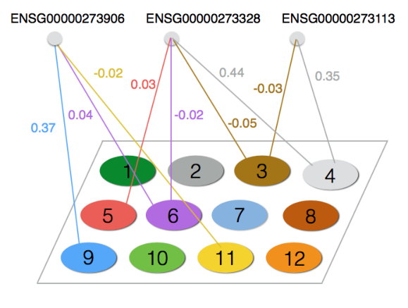
To benchmark LOVE, we used a publicly available RNA-seq dataset of 285 blood platelet samples from patients with different malignant tumors (Best et al., 2015). We extracted a small subset of 500 Ensembl genes to test the method. The goal of the benchmarking was to test whether (i) clusters corresponded to biological knowledge, specifically Gene Ontology (GO) functional annotation of the genes (Ashburner et al., 2000), (ii) overlapping clusters corresponded to pleiotropic gene function. LOVE produced twelve overlapping clusters (Table 2) which aligned well with a-priori expectation. Table 2 lists the number of pure genes and the total number of genes in twelve overlapping clusters. Figure 2 shows that each cluster overlaps with the other and also gives us a clear picture on how two clusters possibly overlap. For example, 18 genes belong to both cluster 3 and cluster 11, whereas cluster 2 and cluster 3 have only one common gene. The genes with the same GO biological process, molecular function or cellular component terms tended to be assigned to the same cluster. For example, ENSG00000273906 and ENSG00000273328 are both RNA genes. They were both assigned to the same cluster (cluster 6, Figure 2). However, they were also assigned to other clusters, suggesting they have pleiotropic functions. This suggests that the latent variables used for clustering are likely to have biological significance and can potentially be used for functional discovery for genes with under-explored functions. We found 308 genes with zero expression across all samples. None of them were assigned to any of the 12 estimated clusters, as desired. Indeed, our model not only allows for the existence of pure noise variables $X_{j}=E_{j}$ , but variables with structural zero values as well, as $\Gamma_{jj}=\text{Var}(E_{j})=0$ is permitted. Formally we place them in the pure noise cluster $G_{0}$ , for further scientific scrutiny.

Table 2: Number of pure genes and total number of genes in each group.

	G1	G2	G3	G4	G5	G6	G7	G8	G9	G10	G11	G12
Number of pure genes	2	2	2	4	2	10	2	2	2	4	2	15
Total number of genes	58	35	67	105	80	104	28	43	44	74	94	108

Refer to caption — Fig 2: Left panel: Number of genes overlapped in different groups. The nodes represent 12 groups with the same labels and sizes as those in Table 2. The number shown on the edge between two nodes represents the number of genes shared by the two groups, which corresponds to the width of that edge. Right panel: Illustration of three genes ENSG00000273906, ENSG00000273328 and ENSG00000273113 and their allocation matrix relative to 12 groups. For instance, the $j$ th gene ENSG00000273906 belongs to groups 6, 9 and 11 with $\widehat{A}_{j6}=0.04,\widehat{A}_{j9}=0.37,\widehat{A}_{j11}=-0.02$ .

Acknowledgements

We thank the referees for their many insightful and helpful suggestions. We are grateful to Jishnu Das for help with the interpretation of our data analysis results. Bunea and Wegkamp were supported in part by NSF grant DMS 1712709. Bing was supported in part by NSF grant DMS-1407600.

Supplementary Material

Supplement to “Adaptive Estimation in Structured Factor Models with Applications to Overlapping Clustering”:
(doi: COMPLETED BY THE TYPESETTER). The supplementary document includes the proofs and additional numerical results.

A Appendix

A.1 Proofs of the results from Section 2

We begin by stating and proving two lemmata that are crucial for the main results of this section. All results are proved under the condition that model 1.1 and (i) - (iii) hold.

Lemma 8.

For any $a\in[K]$ and $i\in I_{a}$ , we have

(a)

$|\Sigma_{ij}|=C_{aa}$ for all $j\in I_{a}$ ,
(b)

$|\Sigma_{ij}|<C_{aa}$ for all $j\not\in I_{a}$ .

For given $i\in[p]$ , we define the set $s(i):=\{1\leq a\leq K:A_{ia}\neq 0\}$ . For any $i\in I_{a}$ and $j\neq i$ , we have

$\displaystyle\|\Sigma_{ij}\|$	$\displaystyle=$	$\displaystyle\left\|\sum_{a\in s(i)}A_{ia}\Bigl(\sum_{b\in s(j)}A_{jb}C_{ab}\Bigr)\right\|$
	$\displaystyle=$	$\displaystyle\Biggl\|\sum_{b\in s(j)}A_{jb}C_{ab}\Biggr\|\text{ from the definition of $I_{a}$}$
	$\displaystyle\leq$	$\displaystyle\sum_{b\in s(j)}\|A_{jb}\|\cdot\max_{b\in s(i)}\|C_{ab}\|$
	$\displaystyle\leq$	$\displaystyle C_{aa}\text{ using conditions (i) and (iii)}.$

Furthermore, using conditions (i) and (iii), we observe that we have equality in the above display for $j\in I_{a}$ , and strict inequality for $j\not\in I_{a}$ , which proves the lemma. ∎

Lemma 9.

We have

(a)

$S_{i}\cap I\neq\varnothing$ , for any $i\in[p]$ ,
(b)

$S_{i}\cup\{i\}=I_{a}$ and $M_{i}=C_{aa}$ , for any $i\in I_{a}$ and $a\in[K]$ ,

where $M_{i}$ and $S_{i}$ are defined in (2.2) and (2.3), respectively.

Lemma 8 implies that, for any $i\in I_{a}$ , $M_{i}=C_{aa}$ and $S_{i}=I_{a}\setminus\{i\}$ , which proves part (b).
From the result of part (b), it remains to show $S_{i}\cap I\neq\varnothing$ for any $i\notin I$ . Let $i\notin I$ be fixed. We have

	$\displaystyle M_{i}$	$\displaystyle=$	$\displaystyle\max_{j\neq i}\|\Sigma_{ij}\|\ =\ \max_{j\neq i}\left\|\sum_{b\in s(j)}A_{jb}\Biggl(\sum_{a\in s(i)}A_{ia}C_{ab}\Biggr)\right\|$		(A.1)
		$\displaystyle\leq$	$\displaystyle\max_{j\neq i}\max_{b\in s(j)}\left\|\sum_{a\in s(i)}A_{ia}C_{ab}\right\|\ =\ \max_{j\neq i}\Biggl\|\sum_{a\in s(i)}A_{ia}C_{ab^{*}}\Biggr\|$		(A.1)

for some $b^{*}\in[K]$ . A direct computation yields $|\Sigma_{ij}|=|\sum_{a\in s(i)}A_{ia}C_{ab^{*}}|$ for any $j\in I_{b^{*}}$ , that is, the maximum $M_{i}$ of $|\Sigma_{ij}|$ is achieved at all $j\in I_{b^{*}}$ . Since $I_{b^{*}}\not=\varnothing$ by condition (ii), this completes the proof of claim (a). ∎

Proof of Theorem 1. We have all the necessary ingredients to proceed with the proof of the main result of this section.

Proof of (a). We first show the sufficiency part. Consider any $i\in[p]$ with $M_{i}=M_{j}$ for all $j\in S_{i}$ . Part (a) of Lemma 9 states that there exists a $j\in I_{a}\cap S_{i}$ for some $a\in[K]$ . For this $j\in I_{a}$ , we have $M_{j}=C_{aa}$ from part (b) of Lemma 9. Invoking our premise $M_{j}=M_{i}$ as $j\in S_{i}$ , we conclude that $M_{i}=C_{aa}$ , that is, $\max_{k\neq i}|\Sigma_{ik}|=C_{aa}$ . By Lemma 8, the maximum is achieved for any pair $i,k\in I_{a}$ . However, if $i\not\in I_{a}$ , we have that $|\Sigma_{ik}|<C_{aa}$ for all $k\neq i$ . Hence $i\in I_{a}$ and this concludes the proof of the sufficiency part.

It remains to prove the necessity part. Let $i\in I_{a}$ for some $a\in[K]$ and $j\in S_{i}$ . Lemma 9 implies that $j\in I_{a}$ and $M_{i}=C_{aa}$ . Since $j\in S_{i}$ , we have $|\Sigma_{ij}|=M_{i}=C_{aa}$ , while $j\in I_{a}$ yields $|\Sigma_{jk}|\leq C_{aa}$ for all $k\neq j$ , and $|\Sigma_{jk}|=C_{aa}$ for $k\in I_{a}$ , as a result of Lemma 8. Hence, $M_{j}=\max_{k\neq j}|\Sigma_{jk}|=C_{aa}=M_{i}$ for any $j\in S_{i}$ , which proves our claim.

Proof of (b). We start with the following constructive approach. Let $N=[p]$ be the set of all variable indices and $O=\varnothing$ . Let $M_{i}$ and $S_{i}$ be defined in (2.2) and (2.3), respectively.

(1)
Choose $i\in N$ and calculate $S_{i}$ and $M_{i}$ .
- (a)
  
  If $M_{i}=M_{j}$ , for all $j\in S_{i}$ , set $I^{(i)}:=S_{i}\cup\{i\}$ , $O=O\cup\{i\}$ and $N=N\setminus I^{(i)}$ .
- (b)
  
  Otherwise, replace $N$ by $N\setminus\{i\}$ .
(2)

Repeat step (1) until $N=\varnothing$ .

We show that $\{I^{(i)}:\ {i\in O}\}=\mathcal{I}.$ Let $i\in O$ be arbitrary fixed. By (a), we have $i\in I$ . Thus, there exists $a\in[K]$ such that $i\in I_{a}$ . By Lemma 9, $i\in I_{a}$ implies $I_{a}=S_{i}\cup\{i\}=I^{(i)}$ . On the other hand, let $a\in[K]$ be arbitrary fixed. By condition (ii), there exists at least one $j\in I_{a}$ . Once again, by part (b) of Lemma 9, if $j\in I_{a}$ , then $S_{j}\cup\{j\}=I_{a}$ , that is, $I^{(j)}=I_{a}$ .∎

Proof of Theorem 2

Theorem 1 shows that $\Sigma$ uniquely defines $I$ and its partition $\mathcal{I}$ , up to permutation of labels. Given $I$ and its partition $\mathcal{I}=\{I_{1},\ldots,I_{K}\}$ , for any $i\in I$ , there exists a unique $1\leq a\leq K$ such that $i\in I_{a}$ . Then we set $|A_{i\cdot}|=e_{a}$ , the canonical basis vector in $\mathbb{R}^{K}$ that contains 1 in position $a$ and is zero otherwise. Thus, the $|I|\times K$ matrix $A_{I}$ with rows $A_{i\cdot}$ is uniquely defined up to multiplication with a signed permutation matrix $P$ .

We show below that $A_{J}$ is also identifiable up to a signed permutation matrix. We begin by observing that, for each $i\in I_{k}$ , for some $k\in[K]$ , and any $j\in J$ , Model 1.1 implies

\Sigma_{ij}=\sum_{a\in s(i)}\sum_{b\in s(j)}A_{ia}A_{jb}C_{kb}=A_{ik}\sum_{b\in s(j)}A_{jb}C_{kb}

and since $A_{ik}^{2}=1$ , we obtain

A_{ik}\Sigma_{ij}=C_{k\cdot}^{T}A_{j\cdot}

and, after averaging over all $i\in I_{k}$ ,

C_{k\cdot}^{T}A_{j\cdot}=\frac{1}{|I_{k}|}\sum_{i\in I_{k}}A_{ik}\Sigma_{ij}.

Repeating this for every $k\in[K]$ , we obtain the formula

\displaystyle CA_{j\cdot}

\displaystyle=

\displaystyle\left(\frac{1}{|I_{1}|}\sum_{i\in I_{1}}A_{i1}\Sigma_{ij},\ldots,\frac{1}{|I_{K}|}\sum_{i\in I_{K}}A_{iK}\Sigma_{ij}\right)^{T}:=\theta^{j}.

The covariance matrix $C$ can be uniquely constructed from $\Sigma$ via

\displaystyle C_{aa}

\displaystyle=

\displaystyle\frac{1}{|I_{a}|(|I_{a}|-1)}\sum_{i,j\in I_{a},i\neq j}|\Sigma_{ij}|

for any $a\in[K]$ , and

\displaystyle C_{ab}

\displaystyle=

\displaystyle\frac{1}{|I_{a}||I_{b}|}\sum_{i\in I_{a},j\in I_{b}}A_{ia}A_{jb}\Sigma_{ij}

for $a,b\in[K]$ with $a\neq b$ . Notice that $\min_{a\in[K]}|I_{a}|\geq 2$ , which is part of our model requirement (ii), is needed for the construction of $C_{aa}$ . Since the covariance matrix $C$ is assumed to be positive definite, $A_{j\cdot}=C^{-1}\theta^{j}$ , for each $j\in J$ , which shows that $A_{J}$ can be determined uniquely from $\Sigma$ up to a signed permutation. Therefore, $A_{J}$ is identifiable which concludes the proof. ∎

A.2 Proofs of the results from Section 4.1

The proof of Theorem 3 will repeatedly use Lemma 10, stated and proved below. Let

\widehat{M}_{i}:=\max_{j\in[p]\setminus\{i\}}|\widehat{\Sigma}_{ij}|.

(A.2)

Lemma 10.

Under the conditions in Theorem 3, for any $i\in I_{a}$ with some $a\in[K]$ , the following inequalities hold on the event $\mathcal{E}$ :

$\displaystyle\Bigl\|\|\widehat{\Sigma}_{ij}\|-\|\widehat{\Sigma}_{ik}\|\Bigr\|\leq 2\delta,$	$\displaystyle\quad\text{ for all }j,k\in I_{a}\setminus\{i\}\text{ and }j\neq k;$	(A.3)
$\displaystyle\|\widehat{\Sigma}_{ij}\|-\|\widehat{\Sigma}_{ik}\|>2\delta,$	$\displaystyle\quad\text{ for all }j\in I_{a}\setminus\{i\},\ k\notin(I_{a}\cup J_{1}^{a});$	(A.4)
$\displaystyle\|\widehat{\Sigma}_{ij}\|-\|\widehat{\Sigma}_{ik}\|<2\delta,$	$\displaystyle\quad\text{ for all }j\in J_{1}^{a}\text{ and }k\in I_{a}\setminus\{i\}.$	(A.5)

For any $i\in J_{1}^{a}$ , we have

\widehat{M}_{i}-|\widehat{\Sigma}_{ij}|\leq 2\delta,\qquad\text{for any }j\in I_{a}.

(A.6)

For the entire proof, we work on the event $\mathcal{E}$ defined in (4.1). To prove (A.3), we observe that, for any $i,j,k\in I_{a}$ , $\Sigma_{ij}=\Sigma_{ik}=C_{aa}$ by Lemma 8, whence

\displaystyle\Bigl||\widehat{\Sigma}_{ij}|-|\widehat{\Sigma}_{ik}|\Bigr|

\displaystyle\leq

\displaystyle\bigl||\Sigma_{ij}|-|\Sigma_{ik}|\bigr|+2\delta=2\delta.

To prove (A.4), we first observe that, for any $j\in I_{a}$ , $|\Sigma_{ij}|=C_{aa}$ by Lemma 8, whence

|\widehat{\Sigma}_{ij}|\overset{\mathcal{E}}{\geq}C_{aa}-\delta.

(A.7)

Next, we notice that, for any $\ell\in[p]$ ,

	$\displaystyle\|\Sigma_{i\ell}\|$	$\displaystyle\ =\ \Biggl\|\sum_{b=1}^{K}A_{\ell b}C_{ab}\Biggr\|=\Biggl\|A_{\ell a}C_{aa}+\sum_{b\neq a}A_{\ell b}C_{ab}\Biggr\|$
		$\displaystyle\overset{(iii)}{\leq}\ \|A_{\ell a}\|C_{aa}+(1-\|A_{\ell a}\|)(C_{aa}-\nu)\ =\ C_{aa}-(1-\|A_{\ell a}\|)\nu.$		(A.8)

For any $j\in I_{a}$ and $k\in[p]\setminus(I_{a}\cup J_{1}^{a})$ , the definition of $J_{1}$ implies $|A_{ka}|\leq 4\delta/\nu$ , hence

|\widehat{\Sigma}_{ik}|\overset{\mathcal{E}}{\leq}|\Sigma_{ik}|+\delta\overset{(\ref{display7})}{\leq}C_{aa}-(1-|A_{ka}|)\nu+\delta\leq C_{aa}-\nu+5\delta,

so that

\displaystyle|\widehat{\Sigma}_{ij}|-|\widehat{\Sigma}_{ik}|\overset{\mathcal{E}}{\geq}|\Sigma_{ij}|-\delta-|\widehat{\Sigma}_{ik}|\geq|\Sigma_{ij}|-C_{aa}+\nu-6\delta>2\delta,

by using $\nu>8\delta\cdot(\|C\|_{\infty}/\nu)\geq 8\delta$ . To prove (A.5), observe that, for any $j\in J_{1}^{a}$ and $k\in I_{a}\setminus\{i\}$ ,

|\widehat{\Sigma}_{ij}|\overset{(\ref{display7})}{\leq}C_{aa}-(1-|A_{ja}|)\nu+\delta<C_{aa}+\delta=|\Sigma_{ik}|+\delta\overset{\mathcal{E}}{\leq}|\widehat{\Sigma}_{ik}|+2\delta.

So far, we have proved (A.3) - (A.5) and it remains to show (A.6). For any $i\in J_{1}^{a}$ , we have, for some $c\in[K]$ ,

	$\displaystyle\widehat{M}_{i}$	$\displaystyle\overset{\mathcal{E}}{\leq}\max_{k\in[p]\setminus{i}}\|\Sigma_{ik}\|+\delta\overset{(\ref{display2})}{=}\Biggl\|\sum_{b=1}^{K}A_{ib}C_{bc}\Biggr\|+\delta$
		$\displaystyle\overset{(\ast)}{\leq}\Biggl\|\sum_{b=1}^{K}A_{ib}C_{ba}\Biggr\|+\delta=\|\Sigma_{ij}\|+\delta\overset{\mathcal{E}}{\leq}\|\widehat{\Sigma}_{ij}\|+2\delta.$

It remains to show that inequality $(\ast)$ holds, for any $c\neq a$ . On the one hand, we have

\Biggl|\sum_{b=1}^{K}A_{ib}C_{bc}\Biggr|\leq|A_{ia}||C_{ac}|+(1-|A_{ia}|)C_{cc}\overset{({iii})}{\leq}|A_{ia}|(C_{aa}-\nu)+(1-|A_{ia}|)C_{cc},

while on the other hand, we find

\Biggl|\sum_{b=1}^{K}A_{ib}C_{ab}\Biggr|\overset{({iii})}{\geq}|A_{ia}||C_{aa}|-(1-|A_{ia}|)(C_{aa}-\nu).

Combining the preceding two display yields

\Biggl|\sum_{b=1}^{K}A_{ib}C_{ab}\Biggr|-\Biggl|\sum_{b=1}^{K}A_{ib}C_{bc}\Biggr|\geq\nu-(1-|A_{ia}|)(C_{aa}+C_{cc}).

The term on the right is positive, since condition (4.7) guarantees that

\nu>\frac{4\delta}{\nu}(C_{aa}+C_{cc})\geq(1-|A_{ia}|)(C_{aa}+C_{cc}),

where the last inequality is due to the definition of $J_{1}$ . This concludes the proof. ∎Lemma 10 remains valid under the conditions of Remark 3 in which case $J_{1}=\varnothing$ and we only need $\nu>4\delta$ to prove (A.4).

Proof of Theorem 3. We work on the event $\mathcal{E}$ throughout the proof. Without loss of generality, we assume that the label permutation $\pi$ is the identity. We start by pointing out that the following three claims are sufficient to prove (a) - (c). Let $\widehat{I}^{(i)}$ be defined in step 4 of Algorithm 1.

(1)

For any $i\in J\setminus J_{1}$ , we have $Pure(i)=False$ .
(2)

For any $i\in I_{a}$ and $a\in[K]$ , we have $Pure(i)=True$ , $I_{a}\subseteq\widehat{I}^{(i)}$ and $\widehat{I}^{(i)}\setminus I_{a}\subseteq J_{1}^{a}$ .
(3)

For any $i\in J_{1}^{a}$ and $a\in[K]$ , we have $I_{a}\subseteq\widehat{I}^{(i)}$ .

If we can prove these claims, then (1) implies that none of variables in $J\setminus J_{1}$ will be selected in any set of $\widehat{\mathcal{I}}$ via $i\in J\setminus J_{1}$ . (2) implies that for any $a\in[K]$ , there exists $\widehat{I}_{a}$ such that $I_{a}\subseteq\widehat{I}_{a}$ and $\widehat{I}_{a}\setminus I_{a}\subseteq J_{1}^{a}$ . Moreover, this together with Merge in Algorithm 1 prevents $\widehat{I}_{a}$ from selecting any variable from $[p]\setminus(I_{a}\cup J_{1}^{a})$ . Finally, (3) guarantees that none of pure variables will be excluded by any $i\in J_{1}$ in the Merge step. Thus, $\widehat{K}=K$ and $\widehat{\mathcal{I}}=\{\widehat{I}_{1},\ldots,\widehat{I}_{K}\}$ is the desired partition. Therefore, in the following we proceed to prove (1) - (3).

To prove (1), let $i\in J\setminus J_{1}$ be fixed. We first prove that $Pure(i)=False$ when $\widehat{I}^{(i)}\cap I\neq\varnothing$ . It suffices to show that, there exists $j\in\widehat{I}^{(i)}$ such that the following does not hold

\widehat{M}_{j}-|\widehat{\Sigma}_{ij}|\leq 2\delta.

(A.9)

Let $\widehat{I}^{(i)}\cap I\neq\varnothing$ , so there exists $j\in I_{b}\cap\widehat{I}^{(i)}$ for some $b\in[K]$ . For such $j$ , we have $|\Sigma_{ij}|=|\sum_{a=1}^{K}A_{ia}C_{ab}|$ and

|\widehat{\Sigma}_{ij}|\overset{\mathcal{E}}{\leq}\Biggl|\sum_{a=1}^{K}A_{ia}C_{ab}\Biggr|+\delta\overset{({iii})}{\leq}|A_{ib}|C_{bb}+(1-|A_{ib}|)(C_{bb}-\nu)+\delta<C_{bb}-3\delta,

(A.10)

using the definition of $J_{1}$ to justify the last inequality. On the other hand, since $j\in I_{b}$ , part (b) of Lemma 9 implies

\widehat{M}_{j}=\max_{k\in[p]\setminus\{i\}}|\widehat{\Sigma}_{jk}|\overset{\mathcal{E}}{\geq}\max_{k\in[p]\setminus\{i\}}|\Sigma_{jk}|-\delta=C_{bb}-\delta.

(A.11)

Combining (A.10) with (A.11) gives $\widehat{M}_{j}-|\widehat{\Sigma}_{ij}|>2\delta.$ This shows that for any $i\in J\setminus J_{1}$ , if $\widehat{I}^{(i)}\cap I\neq\varnothing$ , then $Pure(i)=False$ . Therefore, to complete the proof of (1), we show $\widehat{I}^{(i)}\cap I=\varnothing$ is impossible when $i\in J\setminus J_{1}$ under our assumptions. If $\widehat{I}^{(i)}\cap I=\varnothing$ , then there exists some $j\in J\cap\widehat{I}^{(i)}$ and

|\Sigma_{ij}|=\left|\sum_{b=1}^{K}\sum_{a=1}^{K}A_{ia}A_{jb}C_{ab}\right|\leq\max_{1\leq b\leq K}\left|\sum_{a=1}^{K}A_{ia}C_{ab}\right|=\left|\sum_{a=1}^{K}A_{ia}C_{ab^{*}}\right|=|\Sigma_{ik}|

for some $b^{*}\in[K]$ and any $k\in I_{b^{*}}$ (the set $I_{b^{*}}$ is non-empty by condition (ii)). Therefore,

\displaystyle|\widehat{\Sigma}_{ij}|-|\widehat{\Sigma}_{ik}|

\displaystyle\overset{\mathcal{E}}{\leq}

\displaystyle|\Sigma_{ij}|-|\Sigma_{ik}|+2\delta\quad\leq\quad 2\delta

However, since $\widehat{I}^{(i)}\cap I=\varnothing$ and $k\in I_{b^{*}}$ , we know $k\notin\widehat{I}^{(i)}$ , which implies

\displaystyle|\widehat{\Sigma}_{ij}|-|\widehat{\Sigma}_{ik}|>2\delta,

from Step 4 of Algorithm 1. The last two displays contradict each other, and we conclude that, for any $i\in J\setminus J_{1}$ , $\widehat{I}^{(i)}\cap I\neq\varnothing$ .

To prove (2), let $i\in I_{a}$ be arbitrarily fixed with some $a\in[K]$ . We first show that $Pure(i)=True$ . From steps 7 - 8 of Algorithm 1, it suffices to show that, for any $j\in\widehat{I}^{(i)}$ , (A.9) holds. From (A.4) in Lemma 10, given Step 4 of Algorithm 1, we know that, for any $j\in\widehat{I}^{(i)}$ , $j\in I_{a}\cup J_{1}^{a}$ . Thus, we write $\widehat{I}^{(i)}=(\widehat{I}^{(i)}\cap I_{a})\cup(\widehat{I}^{(i)}\cap J_{1}^{a})$ . For any $j\in\widehat{I}^{(i)}\cap I_{a}$ , by the same reasoning, $\widehat{M}_{j}$ is achieved by some element in either $I_{a}$ or $J_{1}^{a}$ . For both cases, since $i,j\in I_{a}$ and $i\neq j$ , (A.3) and (A.5) in Lemma 10 guarantee that (A.9) holds. On the other hand, for any $j\in\widehat{I}^{(i)}\cap J_{1}^{a}$ , (A.6) in Lemma 10 implies that (A.9) still holds. Thus, we have shown that, for any $i\in I_{a}$ , $Pure(i)=True$ . To show $I_{a}\subseteq\widehat{I}^{(i)}$ , let any $j\in I_{a}\setminus\{i\}$ and observe that $\widehat{M}_{i}$ can only be achieved by indices in $I_{a}\cup J_{1}^{a}$ . In both cases, (A.3) and (A.5) imply $j\in\widehat{I}^{(i)}$ . Thus, $I_{a}\subseteq\widehat{I}^{(i)}$ . Finally, $\widehat{I}^{(i)}\setminus I_{a}\subseteq J_{1}^{a}$ follows immediately from (A.4).

We conclude the proof by noting that (3) immediately follows from (A.6). ∎

A.3 Proofs of the results from Section 4.2

We divide the proof of Theorem 4 into three steps:
Step 1. We show that there exists a signed permutation $\widehat{P}$ such that the columns of $\widehat{A}_{I}$ aligns with those of $A_{I}$ in terms of label and sign, as detailed in Lemma 11;
Step 2. We write $\bar{A}=A\widehat{P}$ , and prove first the error bounds for $\widehat{A}_{\widehat{I}}-\bar{A}_{\widehat{I}}$ ;
Step 3. We prove the error bounds for $\widehat{A}-\bar{A}=\widehat{A}-A\widehat{P}$ , with the same $\widehat{P}$ , which further implies that $\widehat{P}$ aligns the columns of $\widehat{A}$ and $A$ .

Lemma 11.

Under conditions of Theorem 4, there exists a signed permutation matrix $Q$ such that $\bar{A}=AQ$ satisfies that $\mathop{\mathrm{sign}}(\bar{A}_{ia})=\mathop{\mathrm{sign}}(\widehat{A}_{ia})$ for any $i\in\widehat{I}_{a}$ with each $a\in[K]$ .

Theorem 3 guarantees $\widehat{K}=K$ , $I\subseteq\widehat{I}\subseteq I\cup J_{1}$ and $I_{\pi(a)}\subseteq\widehat{I}_{a}\subseteq I_{\pi(a)}\cup J_{1}^{\pi(a)}$ , with high probability, for any $a\in[K]$ and some label permutation $\pi$ . Let us write $Q=Q_{1}Q_{2}$ , with the unsigned permutation matrix $Q_{1}$ which relabels the columns of $A_{I}$ according to those of $\widehat{A}_{I}$ , and with $Q_{2}=\textrm{diag}(q_{1},\ldots,q_{K})$ with $q_{a}\in\{+1,-1\}$ for each $a\in[K]$ .

Denoting $\widecheck{A}=AQ_{1}$ , we proceed to show that, for each $a\in[K]$ , $\mathop{\mathrm{sign}}(\widehat{A}_{ia})=\mathop{\mathrm{sign}}(\widecheck{A}_{ia})\cdot q_{a}$ holds for any $i\in\widehat{I}_{a}$ , in which case each $q_{a}$ can be uniquely constructed. Since $\widehat{I}_{a}\subseteq I_{\pi(a)}\cup J_{1}^{\pi(a)}$ , it suffices to prove that, for any $a\in[K]$ ,

\frac{\mathop{\mathrm{sign}}(\widehat{A}_{ia})}{\mathop{\mathrm{sign}}(\widecheck{A}_{ia})}=\frac{\mathop{\mathrm{sign}}(\widehat{A}_{ja})}{\mathop{\mathrm{sign}}(\widecheck{A}_{ja})},\quad\text{ for any }i,j\in I_{\pi(a)}\text{ or }i,j\in J_{1}^{\pi(a)}\text{ with }i\neq j.

(A.12)

From the definition of $A_{I}$ and the way we construct $\widehat{A}_{I}$ , for any $i,j\in I_{\pi(a)}$ or $i,j\in J_{1}^{\pi(a)}$ , we consider the following two cases:

If $\mathop{\mathrm{sign}}({A_{i{\pi(a)}}})=\mathop{\mathrm{sign}}(A_{j{\pi(a)}})$ , this implies $\mathop{\mathrm{sign}}(\widecheck{A}_{ia})=\mathop{\mathrm{sign}}(\widecheck{A}_{ja})$ . To show $\widehat{A}_{ia}=\widehat{A}_{ja}$ , from (3.1), we need to show $i,j\in\widehat{I}_{a}^{1}$ or $i,j\in\widehat{I}_{a}^{2}$ which is equivalent to show $\widehat{\Sigma}_{ij}>0$ . For any $i,j\in I_{\pi(a)}$ or $i,j\in J_{1}^{\pi(a)}$ with $i\neq j$ , display (4.5) gives $|A_{k{\pi(a)}}|\geq 1-4\delta/\nu$ and $\sum_{b\neq{\pi(a)}}|A_{kb}|\leq 4\delta/\nu$ , for $k=i,j$ . Thus, using $\mathop{\mathrm{sign}}(A_{i{\pi(a)}})=\mathop{\mathrm{sign}}(A_{j{\pi(a)}})$ , we have

	$\displaystyle\Sigma_{ij}$	$\displaystyle\ =\ A_{i{\pi(a)}}A_{j{\pi(a)}}C_{\pi(a)\pi(a)}+A_{i\pi(a)}\sum_{c\neq a}A_{jc}C_{\pi(a)c}+A_{j\pi(a)}\sum_{b\neq a}A_{ib}C_{\pi(a)b}$
		$\displaystyle\qquad+\sum_{b,c\neq{\pi(a)}}A_{ib}A_{jc}C_{bc}$
		$\displaystyle\overset{(iii)}{\geq}\ A_{i{\pi(a)}}A_{j{\pi(a)}}C_{\pi(a)\pi(a)}-\|A_{i\pi(a)}\|(1-\|A_{j\pi(a)}\|)(C_{\pi(a)\pi(a)}-\nu)$
		$\displaystyle\qquad-\|A_{j\pi(a)}\|(1-\|A_{i\pi(a)}\|)(C_{\pi(a)\pi(a)}-\nu)-\sum_{b,c\neq{\pi(a)}}A_{ib}A_{jc}C_{bc}$
		$\displaystyle\ \geq\ \left(1-\frac{4\delta}{\nu}\right)^{2}C_{\pi(a)\pi(a)}-\frac{8\delta}{\nu}\cdot\left(1-\frac{4\delta}{\nu}\right)C_{\pi(a)\pi(a)}-\frac{16\delta^{2}}{\nu^{2}}C_{b^{}b^{}}+8\delta$
		$\displaystyle\ \geq\ \left(1+\frac{48\delta^{2}}{\nu^{2}}-\frac{16\delta}{\nu}\right)C_{\pi(a)\pi(a)}-\frac{16\delta^{2}}{\nu^{2}}C_{b^{}b^{}}+8\delta,$

for some $b^{*}\neq\pi(a)$ . Since (4.7) implies $8\delta C_{b^{*}b^{*}}<\nu^{2}$ and $\nu>8\delta$ , on the event $\mathcal{E}$ , we have $\widehat{\Sigma}_{ij}\geq\Sigma_{ij}-\delta>3\delta>0$ .

If $\mathop{\mathrm{sign}}(A_{i{\pi(a)}})\neq\mathop{\mathrm{sign}}(A_{j{\pi(a)}})$ , this gives $\mathop{\mathrm{sign}}(\widecheck{A}_{ia})\neq\mathop{\mathrm{sign}}(\widecheck{A}_{ja})$ . Similarly, to show $\widehat{A}_{ia}\neq\widehat{A}_{ja}$ , we prove $\widehat{\Sigma}_{ij}<0$ . Using the same arguments yields

\displaystyle\widehat{\Sigma}_{kl}\overset{\mathcal{E}}{\leq}\Sigma_{kl}+\delta<-3\delta<0.

Therefore, given $\widehat{\mathcal{I}}=\{\widehat{I}_{a}\}_{a\in[K]}$ , we can construct the signed permutation $\widehat{P}=Q$ which alligns the columns of $A_{I}$ with those of $\widehat{A}_{I}$ . ∎

For ease of notation and without loss of generality, we make the blanket assumption that the signed permutation $\widehat{P}$ is the identity so that $\bar{A}=A$ for the remainder of the proof. We note that the signed permutation $\widehat{P}$ will be the same when estimating each row $A_{j\cdot}$ for $j\in J$ .

Proof of step 2: From the construction of $\widehat{A}_{\widehat{I}}$ and parts (a) - (c) in Theorem 3, we can write, for each $a\in[K]$ , $\widehat{I}_{a}=I_{a}\cup L_{a}$ with $L_{a}:=\widehat{I}_{a}\cap J_{1}^{a}$ . For any $i\in\widehat{I}_{a}$ , the definitions of $I$ and $J_{1}^{a}$ imply $|A_{i{a}}|\geq 1-4\delta/\nu$ . Since Lemma 11 guarantees that $\mathop{\mathrm{sign}}(A_{ia})=\mathop{\mathrm{sign}}(\widehat{A}_{ia})$ , we have

\displaystyle\|\widehat{A}_{\widehat{I}}-{A}_{\widehat{I}}\|_{\infty}=\max_{i\in\widehat{I}}\|\widehat{A}_{i.}-A_{i.}\|_{\infty}\leq\frac{4}{\nu}\delta.

Let $s_{i}=\|A_{i\cdot}\|_{0}$ for $i\in[p]$ . Then, for any $i\in\widehat{I}$ , we have

\displaystyle\bigl\|\widehat{A}_{j\cdot}-\bar{A}_{j\cdot}\bigr\|_{q}\leq\frac{4}{\nu}s_{i}^{1/q}\delta,\qquad 1\leq q\leq\infty.

∎

For Step 3 of the proof of Theorem 4, we will make use of the results of Lemmas 12 and 13, stated here first and proved at the end of this section, in order to preserve the flow of the presentation.

Lemma 12.

Under the conditions of Theorem 4, on the event $\mathcal{E}$ , we have

\|\widehat{C}-C\|_{\infty}\leq 2\delta^{\prime},\qquad\max_{j\in\widehat{J}}\|\widehat{\theta}^{j}-\theta^{j}\|_{\infty}\leq\delta^{\prime},

(A.13)

where $\delta^{\prime}$ is given in (4.8).

Lemma 13.

Under the conditions of Theorem 4, on the event $\mathcal{E}$ , we have $\beta_{a}^{j}=0$ implies $\widehat{\beta}_{a}^{j}=0$ , for any $j\in\widehat{J}$ and $a\in[\widehat{K}]$ .

Proof of Step 3. For each $j\in\widehat{J}$ , recall that $\beta^{j}=C^{-1}\theta^{j}=\Omega\theta^{j}$ since $C$ is invertible. Also recall that $\bar{\beta}^{j}=\widehat{\Omega}\widehat{\theta}^{j}$ . We first show $\|\bar{\beta}^{j}-\beta^{j}\|_{\infty}\leq 5\|\Omega\|_{\infty,1}\delta^{\prime}$ . For notational convenience, we remove all the super indices. From Lemma 12, the following event

\mathcal{E}^{\prime}=\left\{\|\widehat{C}-C\|_{\infty}\leq 2\delta^{\prime},\ \max_{j\in\widehat{J}}\|\widehat{\theta}^{j}-\theta^{j}\|_{\infty}\leq\delta^{\prime}\right\},

is implied by the event $\mathcal{E}=\mathcal{E}_{\delta}$ . On the event $\mathcal{E}^{\prime}$ , the true $\Omega:=C^{-1}$ satisfies the constraint since

\|\Omega\widehat{C}-I\|_{\infty}\ =\ \|\Omega(\widehat{C}-C)\|_{\infty}\ \leq\ \|\widehat{C}-C\|_{\infty}\|\Omega\|_{\infty,1}\ \leq\ 2\delta^{\prime}\|\Omega\|_{\infty,1}.

Then the pair $(\|\Omega\|_{\infty,1},\Omega)$ of $(t,\Omega)$ is feasible. Consequently, the optimality and feasibility of $(\widehat{t},\widehat{\Omega})$ imply

\|\widehat{\Omega}\|_{\infty,1}\leq\widehat{t}\leq\|\Omega\|_{\infty,1},\quad\|\widehat{\Omega}\widehat{C}-I\|_{\infty}\leq 2\delta^{\prime}\widehat{t}\leq 2\delta^{\prime}\|\Omega\|_{\infty,1}.

(A.14)

Then, on the event $\mathcal{E}^{\prime}$ , we obtain

$\displaystyle\\|\bar{\beta}-\beta\\|_{\infty}$	$\displaystyle=$	$\displaystyle\\|\widehat{\Omega}\widehat{\theta}-\widehat{\Omega}\theta+\widehat{\Omega}\theta-\beta\\|_{\infty}$
	$\displaystyle\leq$	$\displaystyle\\|\widehat{\Omega}\\|_{\infty,1}\\|\widehat{\theta}-\theta\\|_{\infty}+\\|\widehat{\Omega}\theta-\beta\\|_{\infty}$
	$\displaystyle\leq$	$\displaystyle\delta^{\prime}\\|\widehat{\Omega}\\|_{\infty,1}+\\|\widehat{\Omega}C\beta-\beta\\|_{\infty}$
	$\displaystyle\leq$	$\displaystyle\delta^{\prime}\\|\Omega\\|_{\infty,1}+\\|\widehat{\Omega}C-I\\|_{\infty}\\|\beta\\|_{1}$
	$\displaystyle\leq$	$\displaystyle\delta^{\prime}\\|\Omega\\|_{\infty,1}+\\|\widehat{\Omega}\widehat{C}-I\\|_{\infty}+\\|\widehat{\Omega}\widehat{C}-\widehat{\Omega}C\\|_{\infty}\quad(\text{since }\\|\beta\\|_{1}\leq 1)$
	$\displaystyle\leq$	$\displaystyle 3\delta^{\prime}\\|\Omega\\|_{\infty,1}+\\|\widehat{\Omega}\\|_{\infty,1}\\|\widehat{C}-C\\|_{\infty}$
	$\displaystyle\leq$	$\displaystyle 5\delta^{\prime}\\|\Omega\\|_{\infty,1}.$

The feasibility of $\widehat{\beta}^{j}$ implies that $\|\widehat{\beta}^{j}-\bar{\beta}^{j}\|_{\infty}\leq\mu$ . By the triangle inequality, we obtain

\displaystyle\|\widehat{\beta}^{j}-\beta^{j}\|_{\infty}

\displaystyle\leq

\displaystyle\|\widehat{\beta}^{j}-\bar{\beta}^{j}\|_{\infty}+\|\bar{\beta}^{j}-\beta^{j}\|_{\infty}\ \leq\ 2\mu,

since $\mu=5\delta^{\prime}\|\Omega\|_{\infty,1}$ . Then following from Lemma 13 and using $\widehat{K}=K$ on the event $\mathcal{E}$ gives

\|\widehat{A}_{j\cdot}-A_{j\cdot}\|_{q}=\left(\sum_{a=1}^{K}|\widehat{\beta}^{j}_{a}-\beta^{j}_{a}|^{q}\right)^{1/q}=\left(\sum_{a\in s_{j}}|\widehat{\beta}^{j}_{a}-\beta^{j}_{a}|^{q}\right)^{1/q}\leq\ 2s_{j}^{1/q}\mu,

for any $1\leq q\leq\infty$ . This completes the proof of the last step and of Theorem 4. ∎

To conclude this section we give below the proofs of the intermediary results used in the proof.

Proof of Lemma 12. On the event $\mathcal{E}$ , we showed that $\widehat{K}=K$ . Then, from the definition of $\widehat{C}_{aa}$ , we have

	$\displaystyle\max_{1\leq a\leq K}\|\widehat{C}_{aa}-C_{aa}\|$	$\displaystyle\ \leq\ \max_{1\leq a\leq K}\frac{1}{\|\widehat{I}_{a}\|(\|\widehat{I}_{a}\|-1)}\sum_{i,j\in\widehat{I}_{a},i\neq j}\bigl\|\|\widehat{\Sigma}_{ij}\|-C_{aa}\bigr\|$
		$\displaystyle\ \overset{\mathcal{E}}{\leq}\ \delta+\frac{1}{\|\widehat{I}_{a}\|(\|\widehat{I}_{a}\|-1)}\sum_{i,j\in\widehat{I}_{a},i\neq j}\bigl\|\|\Sigma_{ij}\|-C_{aa}\bigr\|.$

Theorem 3 states that, on the event $\mathcal{E}$ , $\widehat{I}_{a}=I_{a}\cup L_{a}$ where $L_{a}=\widehat{I}_{a}\cap J_{1}^{a}$ , for any $a\in[K]$ . Therefore, we consider the following three cases:
(1) For any $i,j\in I_{a}$ and $i\neq j$ , Lemma 8 implies $\bigl||\Sigma_{ij}|-C_{aa}\bigr|=0$ .
(2) For any $i\in I_{a}$ and $j\in L_{a}$ , the definition of $J_{1}^{a}$ gives

\displaystyle\bigl||\Sigma_{ij}|-C_{aa}\bigr|\leq\bigl(1-|A_{ja}|\bigr)(2C_{aa}-\nu)\leq\frac{8\delta}{\nu}\|C\|_{\infty}-4\delta.

(3) For any $i,j\in L_{a}$ and $i\neq j$ , since $i,j\in J_{1}^{a}$ , we know $|A_{ka}|\geq 1-4\delta/\nu$ and $\sum_{b\neq a}|A_{kb}|\leq 4\delta/\nu$ , for $k=i,j$ . Thus,

	$\displaystyle\bigl\|\|\Sigma_{ij}\|-C_{aa}\bigr\|$	$\displaystyle\leq\bigl(1-\|A_{ia}\|\|A_{ja}\|\bigr)C_{aa}+\|A_{ia}\|\sum_{c\neq a}\|A_{jc}\|\|C_{ac}\|+\|A_{ja}\|\sum_{b\neq a}\|A_{ib}\|\|C_{ab}\|$
		$\displaystyle\quad+\sum_{b,c\neq a}\|A_{ib}A_{jc}\|C_{bc}$
		$\displaystyle\leq\bigl(1-\|A_{ia}\|\|A_{ja}\|\bigr)C_{aa}+\|A_{ia}\|(1-\|A_{ja}\|)(C_{aa}-\nu)$
		$\displaystyle\quad+\|A_{ja}\|(1-\|A_{ib}\|)(C_{aa}-\nu)+(1-\|A_{ib}\|)(1-\|A_{jc}\|)C_{b^{}b^{}}$
		$\displaystyle\leq\left[1-\left(1-\frac{4\delta}{\nu}\right)^{2}\right]C_{aa}+\frac{8\delta}{\nu}(C_{aa}-\nu)+\frac{16\delta^{2}}{\nu^{2}}C_{b^{}b^{}}$
		$\displaystyle\leq\frac{16\delta}{\nu}\\|C\\|_{\infty}-8\delta,\qquad(\text{by }(\ref{nu})).$

for some $b^{*}\neq a$ , where we use the definition of $J_{1}$ in the third inequality. Therefore, by combining cases (1) - (3), we have

	$\displaystyle\max_{1\leq a\leq K}\|\widehat{C}_{aa}-C_{aa}\|$	$\displaystyle\ \leq\ \delta+\frac{\|I_{a}\|\|L_{a}\|+\|L_{a}\|(\|L_{a}\|-1)}{\|\widehat{I}_{a}\|(\|\widehat{I}_{a}\|-1)}\cdot\left(\frac{16\delta\\|C\\|_{\infty}}{\nu}-8\delta\right)$
		$\displaystyle\ \leq\ \left(\frac{16}{\nu}\\|C\\|_{\infty}-7\right)\delta.$

where the last inequality comes from that $|L_{a}|+|I_{a}|=|\widehat{I}_{a}|$ . For the off-diagonal entries, since $\mathop{\mathrm{sign}}(\widehat{A}_{ia})=\mathop{\mathrm{sign}}(A_{ia})$ , for any $i\in\widehat{I}$ and $a\in[K]$ , we have

\displaystyle\max_{1\leq a,b\leq K,a\neq b}|\widehat{C}_{ab}-C_{ab}|

\displaystyle\leq

\displaystyle\delta+\frac{1}{|\widehat{I}_{a}||\widehat{I}_{b}|}\sum_{i\in\widehat{I}_{a},j\in\widehat{I}_{b}}\bigl||\Sigma_{ij}|-|C_{ab}|\bigr|,

we consider the following three cases:
(1) For any $i\in I_{a},j\in I_{b}$ , we have $|\Sigma_{ij}|-|C_{ab}|=0$ .
(2) For any $i\in I_{a}$ , $j\in J_{1}^{b}$ , we have

\displaystyle\bigl||\Sigma_{ij}|-|C_{ab}|\bigr|\leq(1-|A_{jb}|)|C_{ab}|+\sum_{c\neq b}|A_{jc}||C_{ac}|\leq\frac{8\delta}{\nu}\|C\|_{\infty}-4\delta.

(3) For any $i\in J_{1}^{a}$ , $j\in J_{1}^{b}$ , we obtain

\displaystyle\Sigma_{ij}

\displaystyle=

\displaystyle A_{ia}A_{jb}C_{ab}+A_{ia}\sum_{d\neq b}A_{jd}C_{ad}+\sum_{c\neq a}A_{ic}\sum_{d\in s(j)}A_{jd}C_{cd}.

Thus,

	$\displaystyle\bigl\|\|\Sigma_{ij}\|-\|C_{ab}\|\bigr\|$	$\displaystyle\leq(1-\|A_{ia}\|\|A_{jb}\|)\|C_{ab}\|+\|A_{ia}\|(1-\|A_{jb}\|)\\|C\\|_{\infty}+(1-\|A_{ia}\|)\\|C\\|_{\infty}$
		$\displaystyle\leq\left(\frac{8\delta}{\nu}-\frac{16\delta^{2}}{\nu^{2}}\right)(C_{aa}-\nu)+\left(\frac{8\delta}{\nu}-\frac{16\delta^{2}}{\nu^{2}}\right)\\|C\\|_{\infty}$
		$\displaystyle\leq\frac{16\delta}{\nu}\\|C\\|_{\infty}-8\delta.\qquad(\text{by }\nu<\\|C\\|_{\infty})$

Therefore, combining the three cases gives

	$\displaystyle\max_{1\leq a,b\leq K,a\neq b}\|\widehat{C}_{ab}-C_{ab}\|$	$\displaystyle\leq\delta+\frac{\|I_{a}\|\|L_{b}\|+\|L_{a}\|\|I_{b}\|+2\|L_{a}\|\|L_{b}\|}{2\|\widehat{I}_{a}\|\|\widehat{I}_{b}\|}\cdot\left(\frac{16\delta\\|C\\|_{\infty}}{\nu}-8\delta\right)$
		$\displaystyle\leq\left(\frac{16}{\nu}\\|C\\|_{\infty}-7\right)\delta.$

Combining the diagonal and off-diagonal cases yields

\|\widehat{C}-C\|_{\infty}\ \leq\ \left(\frac{16}{\nu}\|C\|_{\infty}-7\right)\delta\ \leq\ 2\delta^{\prime}

We now proceed to bound $\max_{j\in\widehat{J}}\|\widehat{\theta}^{j}-\theta^{j}\|_{\infty}$ . From $\mathop{\mathrm{sign}}(A_{ia})=\mathop{\mathrm{sign}}(\widehat{A}_{ia})$ for any $i\in\widehat{I}$ , we obtain

\displaystyle\max_{j\in\widehat{J}}\|\widehat{\theta}^{j}-\theta^{j}\|_{\infty}

\displaystyle\leq

\displaystyle\delta+\max_{a\in[K],j\in\widehat{J}}\frac{1}{|\widehat{I}_{a}|}\sum_{i\in\widehat{I}_{a}}\Bigl|\Sigma_{ij}-\sum_{b\in s(j)}A_{jb}C_{ab}\Bigr|.

Since for any $i\in I_{a}$ and any $j\in J$ , $\Sigma_{ij}=\sum_{b\in s(j)}A_{jb}C_{ab}$ , we focus on the case when $i\in L_{a}$ . For any $i\in L_{a}$ and $j\in J$ , (A.1) yields

\displaystyle\sum_{b\in s(j)}A_{jb}C_{ab}-\Sigma_{ij}

\displaystyle=

\displaystyle(1-A_{ia})\sum_{b\in s(j)}A_{jb}C_{ab}-\sum_{c\neq a}A_{ic}\sum_{b\in s(j)}A_{jb}C_{bc},

which, by the definition of $J_{1}$ , implies

		$\displaystyle\left\|\sum_{b\in s(j)}A_{jb}C_{ab}-\Sigma_{ij}\right\|$
		$\displaystyle\qquad\leq(1-\|A_{ia}\|)\|A_{jd}\|\|C_{ad}\|+(1-\|A_{ia}\|)\|A_{jd^{\prime}}\|\|C_{ad^{\prime}}\|\quad(\text{for some }d,d^{\prime}\in[K])$
		$\displaystyle\qquad\leq\frac{4\delta}{\nu}(2\\|C\\|_{\infty}-\nu)\ \leq\ \frac{8\delta}{\nu}\\|C\\|_{\infty}-4\delta.$

Since we have $\widehat{J}\subseteq J$ , we have

\displaystyle\max_{j\in\widehat{J}}\|\widehat{\theta}^{j}-\theta^{j}\|_{\infty}

\displaystyle\leq\delta+\max_{a}\frac{|L_{a}|}{|\widehat{I}_{a}|}\cdot\left(\frac{8}{\nu}\|C\|_{\infty}-4\right)\delta\leq\left(\frac{8}{\nu}\|C\|_{\infty}-3\right)\delta=\delta^{\prime},

which concludes the proof of Lemma 12. ∎

Proof of Lemma 13. Let $j\in\widehat{J}$ be arbitrarily fixed and $\widehat{\beta}^{j}$ be the optimal solution of (3.11) with $\mu=5\|\Omega\|_{\infty,1}\delta^{\prime}$ . For simplicity, we remove the super indices. Starting with the following Karush-Kuhn-Tucker condition:

\displaystyle\mathop{\mathrm{sign}}(\widehat{\beta}_{a})+\lambda_{a}\mathop{\mathrm{sign}}(\widehat{\beta}_{a}-\bar{\beta}_{a})=0,

(A.15)

subject to

\lambda_{a}(|\widehat{\beta}_{a}-\bar{\beta}_{a}|-\mu)=0,\quad\lambda_{a}\geq 0,\quad\text{for }a=\{1,\ldots,K\},

(A.16)

we obtain

0=\mathop{\mathrm{sign}}(\widehat{\beta}_{a})\left(\widehat{\beta}_{a}-\bar{\beta}_{a}\right)+\lambda_{a}\left|\widehat{\beta}_{a}-\bar{\beta}_{a}\right|\overset{(\ref{kkt2})}{=}\mathop{\mathrm{sign}}(\widehat{\beta}_{a})\left(\widehat{\beta}_{a}-\bar{\beta}_{a}\right)+\lambda_{a}\mu,

(A.17)

by multiplying both sides of (A.15) by $\widehat{\beta}_{a}-\bar{\beta}_{a}$ . In what follows we prove that if $\beta_{a}=0$ , for some $a$ , then $\widehat{\beta}_{a}=0$ . Since this is true when $\lambda_{a}=0$ from (A.15), we only consider when $\lambda_{a}\neq 0$ . Note this implies $|\widehat{\beta}_{a}-\bar{\beta}_{a}|=\mu$ from (A.16). If we assume $\widehat{\beta}_{a}>0$ , then (A.17) gives

\bar{\beta}_{a}-\widehat{\beta}_{a}=\lambda_{a}\mu.

Since $|\widehat{\beta}_{a}-\bar{\beta}_{a}|=\mu,$ we further obtain $\lambda_{a}=1$ and

\bar{\beta}_{a}=\mu+\widehat{\beta}_{a}>\mu.

(A.18)

Recall that $\|\beta-\bar{\beta}\|_{\infty}\leq\mu.$ This implies $\bar{\beta}_{a}\leq\mu+|\beta_{a}|=\mu$ , which contradicts (A.18), so $\widehat{\beta}_{a}$ cannot be strictly positive. Similarly, $\widehat{\beta}_{a}<0$ cannot hold based on similar arguments. Thus, $\widehat{\beta}_{a}=0$ from which we conclude $\textrm{supp}(\widehat{\beta}^{j})\subseteq\textrm{supp}(\beta^{j})$ for any $j\in\widehat{J}$ . ∎

Proof of Theorem 5. Estimation of the submatrix $A_{I}$ is as in Step 2 of the proof of Theorem 4. We denote by $\widehat{\beta}_{D}^{j}$ , $j\in\widehat{J}$ , the minimizer of (3.13) under the constraint (3.14). First, we observe that the true $\beta^{j}$ satisfies the constraint (3.14) on the event $\mathcal{E}$ . Indeed,

$\displaystyle\\|\widehat{C}\beta^{j}-\widehat{\theta}^{j}\\|_{\infty}$	$\displaystyle\leq$	$\displaystyle\\|\widehat{C}\beta^{j}-C\beta^{j}\\|_{\infty}+\\|C\beta^{j}-\widehat{\theta}^{j}\\|_{\infty}$
	$\displaystyle\leq$	$\displaystyle\\|\widehat{C}-C\\|_{\infty}\\|\beta^{j}\\|_{1}+\\|\theta^{j}-\widehat{\theta}^{j}\\|_{\infty}$
	$\displaystyle\leq$	$\displaystyle\\|\widehat{C}-C\\|_{\infty}+\\|\theta^{j}-\widehat{\theta}^{j}\\|_{\infty}$
	$\displaystyle\leq$	$\displaystyle 3\delta^{\prime}=\lambda^{\prime},$

by Lemma 12. Second, this implies, on the event $\mathcal{E}$ , that $\|\widehat{\beta}_{D}^{j}\|_{1}\leq\|\beta^{j}\|_{1}$ and $\widehat{\beta}_{D}^{j}-\beta^{j}$ is in the cone $\mathcal{C}_{S}$ with $S=\textrm{supp}(\beta^{j})$ by a standard argument. Finally, by the definition of the $\ell_{q}$ -sensitivity of $C$ and the feasibility of $\widehat{\beta}^{j}_{D}$ , we get for $\Delta=\widehat{\beta}_{D}^{j}-\beta^{j}$

	$\displaystyle\\|\Delta\\|_{q}$	$\displaystyle\kappa_{q}(C,s)$
		$\displaystyle\leq\\|C\Delta\\|_{\infty}$
		$\displaystyle\leq\\|C\widehat{\beta}_{D}^{j}-\widehat{\theta}^{j}\\|_{\infty}+\\|\widehat{\theta}^{j}-\theta^{j}\\|_{\infty}\quad(\text{since }\theta^{j}=C\beta^{j})$
		$\displaystyle\leq\\|\widehat{C}\widehat{\beta}_{D}^{j}-\widehat{\theta}^{j}\\|_{\infty}+\\|\widehat{C}-C\\|_{\infty}\\|\widehat{\beta}^{j}_{D}\\|_{1}+\\|\widehat{\theta}^{j}-\theta^{j}\\|_{\infty}$
		$\displaystyle\leq\\|\widehat{C}\widehat{\beta}_{D}^{j}-\widehat{\theta}^{j}\\|_{\infty}+\\|\widehat{C}-C\\|_{\infty}+\\|\widehat{\theta}^{j}-\theta^{j}\\|_{\infty}\quad(\text{since }\\|\widehat{\beta}^{j}_{D}\\|_{1}\leq 1)$
		$\displaystyle\leq 2\lambda^{\prime}$

and the conclusion (4.11) follows. It remains to prove the second inequality (4.12). First, we observe that $\|v\|_{q}\leq\|v\|_{\infty}(2s)^{1/q}$ for all $v\in\mathcal{C}_{S}$ and $s=|S|$ by the following computation:

$\displaystyle\\|v\\|_{q}^{q}$	$\displaystyle\leq$	$\displaystyle\\|v\\|_{1}\\|v\\|_{\infty}^{q-1}$
	$\displaystyle\leq$	$\displaystyle 2\\|v_{S}\\|_{1}\\|v\\|_{\infty}^{q-1}\quad(\text{ since $v\in\mathcal{C}_{S}$})$
	$\displaystyle\leq$	$\displaystyle 2s\\|v\\|_{\infty}^{q}.$

This implies that $\kappa_{q}(C,s)\geq(2s)^{-1/q}\kappa_{\infty}(C,s)$ , and clearly $[\kappa_{\infty}(C,s)]^{-1}\leq\|C^{-1}\|_{\infty,1}$ for all $s\leq K$ , with equality for $s=K$ . Now (4.12) follows from (4.11). ∎

Proof of Theorem 6. Without loss of generality, we assume that $\lambda_{1}(C)<\infty$ , since otherwise the lower bound is trivially zero.
First we construct a set of “hypotheses” of $A$ . Let

\mathcal{M}:=\{v\in\{0,1\}^{K}:d_{H}(0,v)=s\}

where $d_{H}(\cdot)$ denotes the Hamming distance between two binary vectors. Following Lemma A.3 in Rigollet and Tsybakov (2011) when $s\leq 4K/5$ , there exists $\mathcal{M}^{\prime}\subset\mathcal{M}$ such that, for any $w^{(i)}\neq w^{(j)}\in M^{\prime}$ ,

d_{H}\left(w^{(i)},w^{(j)}\right)>s/16,

(A.19)

and

\log|\mathcal{M}^{\prime}|\geq c_{0}s\log(K/s),

(A.20)

for some constant $c_{0}>0$ . We let $w^{(0)}=(0,\ldots,0)\in\mathbb{R}^{K}$ . Then, we choose

A^{(j)}=\begin{bmatrix}B\\ \eta\left(w^{(j)}\right)^{T}\end{bmatrix}\in\mathbb{R}^{p\times K},\quad\text{for each $j=0,1,\ldots,|\mathcal{M}^{\prime}|$,}

(A.21)

where

B=\begin{bmatrix}B_{1}\\ B_{2}\\ \vdots\\ B_{K}\end{bmatrix}\in\mathbb{R}^{(p-1)\times K},\quad B_{k}=\begin{bmatrix}e_{k}^{T}\\ e_{k}^{T}\\ \vdots\\ e_{k}^{T}\end{bmatrix}\in\mathbb{R}^{|I_{k}|\times K},~\text{ for }k\in[K],

(A.22)

and

\eta=\sqrt{c_{0}\sigma^{2}\over 8\lambda_{1}(C)}\sqrt{\frac{\log(K/s)}{n}}.

(A.23)

We use $e_{k}$ to denote the canonical basis of $K$ dimensional space and $\bm{0}$ to denote the zero vector. Note that, for each $B_{k}$ , the only non-zero values are at the $k$ th column. By specifying as above, we choose $\sum_{k=1}^{K}|I_{k}|=p-1$ and consider the $A^{(j)}$ with only one non-pure row. It is easy to verify that $A^{(j)}\in\mathcal{A}_{s}$ for each $j=0,1,\ldots,|\mathcal{M}^{\prime}|$ under (4.13).

We denote by $\mathcal{KL}(\mathbb{P},\mathbb{Q})$ the Kullback-Leibler divergence between two probability distributions $\mathbb{P}$ and $\mathbb{Q}$ . Since we particularize into one choice of $C$ , we write $\mathbb{P}_{A}:=\mathbb{P}_{A,C}$ for simplicity. In order to apply Theorem 2.5 in Tsybakov (2009) to prove (4.14), for fixed $\alpha\in(0,1/8)$ , we need to check the following three conditions:

(a)

$\mathcal{KL}(\mathbb{P}_{A^{(i)}},\mathbb{P}_{A^{(0)}})\leq\alpha\log|\mathcal{M}^{\prime}|$ , for each $i=1,\ldots,|\mathcal{M}^{\prime}|$ .
(b)

For any $0\leq i<j\leq|\mathcal{M}^{\prime}|$ , with some constant $c^{\prime}>0$ ,

$L_{q}\left(A^{(i)},A^{(j)}\right)\geq c^{\prime}s^{1/q}\sqrt{\frac{\log(K/s)}{n}}.$
(c)

$L_{q}(\ \cdot\ )$ satisfies the triangle inequality.

To show (a), since $X\sim N(0,ACA^{T}+\sigma^{2}\bm{I}_{p})$ , invoking Lemma 14 gives

\mathcal{KL}\left(\mathbb{P}_{A^{(i)}},\mathbb{P}_{A^{(0)}}\right)\leq\lambda_{1}(C){n\eta^{2}s\over 2\sigma^{2}}\leq\frac{1}{16}\log|M^{\prime}|,\quad\forall\ i=1,\ldots,|M^{\prime}|,

(A.24)

by using (A.20) and (A.23).

To prove (b), for any $i=1,\ldots,|\mathcal{M}^{\prime}|$ , observe that

L_{q}\left(A^{(i)},A^{(0)}\right)=\eta\|w^{(i)}\|_{q}=s^{1/q}\eta

and, for any $i\neq j$ different from $0$ ,

L_{q}\left(A^{(i)},A^{(j)}\right)=\eta\|w^{(i)}-w^{(j)}\|_{q}\geq(s/16)^{1/q}\eta\geq(s^{1/q}\eta)/16,

by using (A.19). Combining these two and using the expression of $\eta$ yield

\displaystyle L_{q}\left(A^{(i)},A^{(j)}\right)\geq c^{\prime}s^{1/q}\sqrt{\sigma^{2}\over\lambda_{1}(C)}\sqrt{\frac{\log(K/s)}{n}},

(A.25)

for $0\leq i<j\leq|\mathcal{M}^{\prime}|$ .

Finally, we verify (c) by showing that $L_{q}(\cdot)$ satisfies the triangle inequality. Consider $(A,\widetilde{A},\widehat{A})$ and observe that

$\displaystyle L_{q}(A,\widetilde{A})$	$\displaystyle=$	$\displaystyle\min_{P\in\mathcal{H}_{K}}\\|AP-\widetilde{A}\\|_{\infty,q}$
	$\displaystyle=$	$\displaystyle\min_{P,Q\in\mathcal{H}_{K}}\\|AP-\widetilde{A}Q\\|_{\infty,q}$
	$\displaystyle\leq$	$\displaystyle\min_{P,Q\in\mathcal{H}_{K}}\left(\\|AP-\widehat{A}\\|_{\infty,q}+\\|\widehat{A}-\widetilde{A}Q\\|_{\infty,q}\right)$
	$\displaystyle=$	$\displaystyle\min_{P\in\mathcal{H}_{K}}\\|AP-\widehat{A}\\|_{\infty,q}+\min_{Q\in\mathcal{H}_{K}}\\|\widehat{A}-\widetilde{A}Q\\|_{\infty,q}$
	$\displaystyle=$	$\displaystyle L_{q}(A,\widehat{A})+L_{q}(\widetilde{A},\widehat{A}).$

Therefore, we conclude the proof of (4.14) by invoking the Theorem 2.5 in Tsybakov (2009). ∎

Lemma 14.

Assume model (1.1) and $X\sim N_{p}(\bm{0},ACA^{T}+\sigma^{2}\bm{I}_{p})$ . Let $A^{(0)}$ and $A^{(i)}$ be constructed as (A.21) and (A.22), for any $1\leq i\leq M^{\prime}$ with $M^{\prime}$ satisfying (A.20). Let $\mathbb{P}_{A^{(0)}}$ and $\mathbb{P}_{A^{(i)}}$ be the probability densities of $X$ parametrized by $A^{(0)}$ and $A^{(i)}$ , respectively. Then we have

\mathcal{KL}\left(\mathbb{P}_{A^{(i)}},\mathbb{P}_{A^{(0)}}\right)\leq\lambda_{1}(C){n\eta^{2}s\over 2\sigma^{2}}.

(A.26)

From the property of Kullback-Leibler divergence, we only need to verify the case when $n=1$ . We consider arbitrary $A^{(i)}$ constructed as (A.21) and (A.22) for some $0\leq i\leq M^{\prime}$ . For notational simplicity, we write $A=A^{(i)}=(B^{T},\xi)^{T}$ where $\xi=\eta w^{(i)}\in\mathbb{R}^{K}$ . For this $A\in\mathbb{R}^{p\times K}$ , from (A.21) and (A.22), we observe that

\Sigma=ACA^{T}+\Gamma=\begin{bmatrix}BCB^{T}+\sigma^{2}\bm{I}_{p-1}&BC\xi\\ \xi^{T}CB^{T}&\xi^{T}C\xi+\sigma^{2}\end{bmatrix}:=\begin{bmatrix}\Sigma_{11}&\Sigma_{12}\\ \Sigma_{21}&\Sigma_{22}\\ \end{bmatrix}.

Similarly, for any $\widetilde{A}\neq A$ constructed in the same way, we have

\widetilde{\Sigma}=\widetilde{A}C\widetilde{A}^{T}+\sigma^{2}\bm{I}_{p-1}=\begin{bmatrix}BCB^{T}+\Gamma_{B}&BC\widetilde{\xi}\\ \widetilde{\xi}^{T}CB^{T}&\widetilde{\xi}^{T}C\widetilde{\xi}+\sigma^{2}\end{bmatrix}:=\begin{bmatrix}\Sigma_{11}&\widetilde{\Sigma}_{12}\\ \widetilde{\Sigma}_{21}&\widetilde{\Sigma}_{22}\\ \end{bmatrix}

Recall that the Kullback-Leibler divergence between two $p$ -dimensional multivariate normal distributions $\mathcal{N}_{0}:=N_{p}(\bm{0},\Sigma)$ and $\mathcal{N}_{1}:=N_{p}(\bm{0},\widetilde{\Sigma})$ is given by

\mathcal{KL}(\mathbb{P}_{\widetilde{A}},\mathbb{P}_{A})={1\over 2}\left[\mathrm{tr}\left(\Sigma^{-1}\widetilde{\Sigma}\right)-p+\log\left({\det\Sigma}\over\det\widetilde{\Sigma}\right)\right].

(A.27)

By using the formula of the inverse of a block matrix

{\begin{bmatrix}{A}&{B}\\ {C}&{D}\end{bmatrix}}^{-1}\!\!\!={\begin{bmatrix}{A}^{-1}+{A}^{-1}{B}({D}-{CA}^{-1}{B})^{-1}{CA}^{-1}&-{A}^{-1}{B}({D}-{CA}^{-1}{B})^{-1}\\ -({D}-{CA}^{-1}{B})^{-1}{CA}^{-1}&({D}-{CA}^{-1}{B})^{-1}\end{bmatrix}},

for square matrices $A$ and $D$ and non-singular matrices $A$ and $D-CA^{-1}B$ , we have

\Sigma^{-1}=\begin{bmatrix}\Sigma_{11}^{-1}+\Sigma_{11}^{-1}\Sigma_{12}\Sigma_{22\cdot 1}^{-1}\Sigma_{21}\Sigma_{11}^{-1}&-\Sigma_{11}^{-1}\Sigma_{12}\Sigma_{22\cdot 1}^{-1}\\ -\Sigma_{22\cdot 1}^{-1}\Sigma_{21}\Sigma_{11}^{-1}&\Sigma_{22\cdot 1}^{-1}\end{bmatrix}:=\begin{bmatrix}\Omega_{11}&\Omega_{12}\\ \Omega_{21}&\Omega_{22}\end{bmatrix},

with $\Sigma_{22\cdot 1}=\Sigma_{22}-\Sigma_{21}\Sigma_{11}^{-1}\Sigma_{12}$ . This gives

\textrm{tr}\left(\Sigma^{-1}\widetilde{\Sigma}\right)=\underbrace{\textrm{tr}\left(\Omega_{11}\Sigma_{11}+\Omega_{12}(BC\widetilde{\xi})^{T}\right)}_{T_{1}}+\underbrace{\Omega_{21}BC\widetilde{\xi}+\Omega_{22}(\widetilde{\xi}^{T}C\widetilde{\xi}+\sigma^{2})}_{T_{2}}.

We first calculate $T_{1}$ by observing that

$\displaystyle T_{1}$	$\displaystyle=$	$\displaystyle\textrm{tr}\left(\bm{I}_{p-1}+\Sigma_{11}^{-1}\Sigma_{12}\Sigma_{22\cdot 1}^{-1}\Sigma_{21}-\Sigma_{11}^{-1}\Sigma_{12}\Sigma_{22\cdot 1}^{-1}\widetilde{\xi}^{T}CB^{T}\right)$	(A.28)
	$\displaystyle=$	$\displaystyle p-1+\textrm{tr}\left(\Sigma_{11}^{-1}\Sigma_{12}\Sigma_{22\cdot 1}^{-1}\Delta^{T}CB^{T}\right)\qquad\left(\Sigma_{21}=\xi^{T}CB^{T}\right)$
	$\displaystyle=$	$\displaystyle p-1+\Sigma_{22\cdot 1}^{-1}\Delta^{T}CB^{T}\Sigma_{11}^{-1}BC\xi$

where $\Delta:=\xi-\widetilde{\xi}\in\mathbb{R}^{K}$ . On the other hand, we have

\displaystyle T_{2}=\Sigma_{22\cdot 1}^{-1}\left(\widetilde{\xi}^{T}C\widetilde{\xi}+\sigma^{2}-\xi^{T}CB^{T}\Sigma_{11}^{-1}BC\widetilde{\xi}\right).

(A.29)

Since our specification of $A=A^{(0)}$ and $\widetilde{A}=A^{(i)}$ in (A.21) and (A.22) gives $\xi=\bm{0}$ and $\widetilde{\xi}=\eta w^{(i)}$ , it implies $\|\widetilde{\xi}\|^{2}=\eta^{2}s$ and

	$\displaystyle\Sigma_{22\cdot 1}$	$\displaystyle=\xi^{T}C\xi+\sigma^{2}-\xi^{T}CB^{T}\Sigma_{11}^{-1}BC\xi=\sigma^{2},$		(A.30)
	$\displaystyle\widetilde{\Sigma}_{22\cdot 1}$	$\displaystyle=\sigma^{2}+\widetilde{\xi}^{T}\left(C-CB^{T}\Sigma_{11}^{-1}BC\right)\widetilde{\xi}.$

Hence combining (A.28) with (A.29) yields

\textrm{tr}\left(\Sigma^{-1}\widetilde{\Sigma}\right)=p+{\widetilde{\xi}^{T}C\widetilde{\xi}\over\sigma^{2}}\leq p+{\eta^{2}s\over\sigma^{2}}\lambda_{1}(C).

(A.31)

To calculate the determinant of $\Sigma$ and $\widetilde{\Sigma}$ , recall that the inverse formula of a block matrix is

\det{\begin{pmatrix}A&B\\ C&D\end{pmatrix}}=\det(A)\det(D-CA^{-1}B)

for any invertible matrix $A$ . We thus obtain

\det\Sigma=\det\Sigma_{11}\cdot\Sigma_{22\cdot 1},\quad\det\widetilde{\Sigma}=\det\Sigma_{11}\cdot\widetilde{\Sigma}_{22\cdot 1},

from which, the display (A.30) further gives

\log\left({\det\Sigma\over\det\widetilde{\Sigma}}\right)=\log\Sigma_{22\cdot 1}-\log\widetilde{\Sigma}_{22\cdot 1}=\log\sigma^{2}-\log\left(\sigma^{2}+\xi^{T}M\xi\right)

with $M:=C-CB^{T}\Sigma_{11}^{-1}BC$ . It is easy to see that $M$ is positive definite. Indeed, since

\left\|C^{1/2}B^{T}\Sigma_{11}^{-1}BC^{1/2}\right\|_{op}=\left\|(BCB^{T}+\sigma^{2}\bm{I}_{p-1})^{-1}BCB^{T}\right\|_{op}<1,

$\lambda_{\min}(M)>0$ follows from

M=C^{1/2}\left(\bm{I}_{p}-C^{1/2}B^{T}\Sigma_{11}^{-1}BC^{1/2}\right)C^{1/2}

and an application of Weyl’s inequality. This implies

\log\left({\det\Sigma\over\det\widetilde{\Sigma}}\right)<0.

(A.32)

Finally, plugging (A.31) and (A.32) into (A.27) concludes the proof of Lemma 14. ∎

A.4 Proofs for the results from Section 4.3

We first prove the three statements of Theorem 7, then present the proofs of Remark 5. Without loss of generality, we assume that the signed permutation $P$ is identity.

Proof of Theorem 7. We first give the proof for part (a). Then, for ease of the presentation, we prove part (c) first and then part (b).

Proof of part (a). Recall that Lemma 13 immediately implies $\textrm{supp}(\widehat{A}_{\widehat{J}})\subseteq\textrm{supp}(A_{\widehat{J}})$ . In addition, Theorem 3 yields $\widehat{I}_{a}\subseteq I_{a}\cup J_{1}^{a}$ , for any $a\in\widehat{K}$ . From the way we construct $\widehat{A}_{\widehat{I}}$ , we have $\textrm{supp}(\widehat{A}_{\widehat{I}})\subseteq\textrm{supp}(A_{\widehat{I}})$ . Therefore, we have proved $\textrm{supp}(\widehat{A})\subseteq\textrm{supp}(A)$ .

On the other hand, for any $(j,a)\in\textrm{supp}(A_{J_{2}})$ , we know $|\beta^{j}_{a}|>2\mu.$ This and the fact that $\|\widehat{\beta}^{j}-\beta^{j}\|_{\infty}\leq 2\mu$ , immediately gives

|\widehat{\beta}^{j}_{a}|\geq|\beta^{j}_{a}|-\|\widehat{\beta}^{j}-\beta^{j}\|_{\infty}>0,

which implies $\textrm{supp}(A_{J_{2}})\subseteq\textrm{supp}(\widehat{A}_{J_{2}})$ .

To show $\mathop{\mathrm{sign}}(\widehat{A}_{\widehat{S}})=\mathop{\mathrm{sign}}(A_{\widehat{S}})$ , since Lemma 11 guarantees $\mathop{\mathrm{sign}}(\widehat{A}_{ia})=\mathop{\mathrm{sign}}(A_{ia})$ for any $(i,a)\in\widehat{S}$ and $i\in\widehat{I}$ , we focus on any fixed $(j,a)\in\widehat{S}$ and $j\in\widehat{J}$ . First, we consider the case $\widehat{A}_{ja}=\widehat{\beta}_{a}^{j}>0$ . Removing super indices, if $\widehat{\beta}_{a}>0$ , (A.18) gives $\bar{\beta}_{a}>\mu$ . Thus, $\beta_{a}\geq\bar{\beta}_{a}-\|\beta-\bar{\beta}\|_{\infty}>0$ by recalling $\|\beta-\bar{\beta}\|_{\infty}\leq\mu$ . So far, we have shown that, for any $\widehat{A}_{ja}>0$ , $(j,a)\in\widehat{S}$ and $j\in\widehat{J}$ , we have $A_{ja}>0$ . Since the same argument holds for any $\widehat{A}_{ja}<0$ , the proof of $\mathop{\mathrm{sign}}(\widehat{A}_{\widehat{S}})=\mathop{\mathrm{sign}}(A_{\widehat{S}})$ is completed.

Proof of part (c). Recall that, for any $i\in[p]$ and $a\in[K]$ ,

i\in G_{a}\iff A_{ia}\neq 0,\qquad i\in\widehat{G}_{a}\iff\widehat{A}_{ia}\neq 0.

We start our proof by rewriting the equivalent expression of TFPP and TFNP:

	TFPP	$\displaystyle=$	$\displaystyle\frac{\sum_{i\in[p],a\in[K]}1{\{A_{ia}=0,\widehat{A}_{ia}\neq 0\}}}{\sum_{i\in[p],a\in[K]}1{\{A_{ia}=0\}}},$
	TFNP	$\displaystyle=$	$\displaystyle\frac{\sum_{i\in[p],a\in[K]}1{\{A_{ia}\neq 0,\widehat{A}_{ia}=0\}}}{\sum_{i\in[p],a\in[K]}1{\{A_{ia}\neq 0\}}}.$

We first show $\text{TFPP}=0$ . From the result of part (a), we know $\textrm{supp}(\widehat{A})\subseteq\textrm{supp}(A)$ . Thus,

\displaystyle\sum_{i\in[p],a\in[K]}1{\{A_{ia}=0,\widehat{A}_{ia}\neq 0\}}=0,

which implies $\text{TFPP}=0$ .

In order to prove the result of TFNP, observe

\sum_{i\in[p],a\in[K]}1{\{A_{ia}\neq 0\}}=|I|+\sum_{i\in J}s_{i}.

(A.33)

with $s_{i}=\|A_{i.}\|_{0}$ for each $j\in J$ . For given $\widehat{I}$ , we partition $[p]=I\cup J_{1}\cup J_{2}\cup J_{3}=I\cup(L_{1}\cup L_{2})\cup J_{2}\cup J_{3}$ with $L_{1}=\widehat{I}\cap J_{1}$ and $L_{2}=J_{1}\setminus L_{1}$ . Let us consider the set $I\cup L_{1}$ first. Theorem 3 implies $I\cup L_{1}=\widehat{I}$ and $\widehat{I}_{a}\setminus I_{a}\subseteq J_{1}^{a}$ . From the way we construct $\widehat{A}_{\widehat{I}}$ , we have

\sum_{i\in I\cup L_{1},a\in[K]}1{\{A_{ia}\neq 0,\widehat{A}_{ia}=0\}}=\sum_{i\in L_{1},a\in[K]}1{\{A_{ia}\neq 0,\widehat{A}_{ia}=0\}}.

Since the definition of $J_{1}$ implies that, for any $j\in J_{1}^{a}$ and $a\in[K]$ , $|A_{ja}|\geq 1-4\delta/\nu$ and $|A_{jb}|\leq 4\delta/\nu$ , for any $b\neq a$ , this implies

\sum_{a\in[K]}1{\{A_{ia}\neq 0,\widehat{A}_{ia}=0\}}=\sum_{b\neq a}1\{A_{ib}\neq 0\}=t_{i},

for any $i\in J_{1}^{a}\cap L_{1}$ and $a\in[K]$ . Thus, we have

\sum_{i\in I\cup L_{1},a\in[K]}1{\{A_{ia}\neq 0,\widehat{A}_{ia}=0\}}=\sum_{i\in L_{1}}t_{i}.

(A.34)

Next we consider the set $L_{2}$ . On the event $\mathcal{E}$ , for any $i\in J_{1}^{a}\cap L_{2}$ , we have

|\widehat{A}_{ia}|\geq|A_{ia}|-\|\widehat{A}-A\|_{\infty}\geq 1-\frac{4\delta}{\nu}-2\mu>0.

Thus, $\widehat{A}_{ia}\neq 0$ , which implies

\sum_{i\in L_{2},a\in[K]}1{\{A_{ia}\neq 0,\widehat{A}_{ia}=0\}}\leq\sum_{i\in L_{2}}t_{i}.

(A.35)

Then we consider the set $J_{2}$ . Part (a) gives $\textrm{supp}(A_{J_{2}})=\textrm{supp}(\widehat{A}_{J_{2}})$ which yields

\sum_{i\in J_{2},a\in[K]}1{\{A_{ia}\neq 0,\widehat{A}_{ia}=0\}}=0.

(A.36)

Finally, we consider the set $J_{3}$ . By examining the proof of Part (a), it is easy to verify that $\widehat{A}_{ja}\neq 0$ if $|A_{ja}|\geq(2\mu)\vee(4\delta/\nu)$ , for any $j\in J_{3}$ and $a\in[K]$ . Thus,

\sum_{i\in J_{3},a\in[K]}1{\{A_{ia}\neq 0,\widehat{A}_{ia}=0\}}\leq\sum_{i\in J_{3}}t_{i}.

(A.37)

At last, combining (A.33) - (A.37) gives

\displaystyle\textrm{TFNP}=\frac{\sum_{i\in[p],a\in[K]}1{\{A_{ia}\neq 0,\widehat{A}_{ia}=0\}}}{\sum_{i\in[p],a\in[K]}1{\{A_{ia}\neq 0\}}}

\displaystyle\leq\frac{\sum_{j\in J_{1}\cup J_{3}}t_{j}}{|I|+\sum_{j\in J}s_{j}}.

Proof of part (b). Similarly, we can express $\textrm{GFPP}(\widehat{G}_{a})$ and $\textrm{GFNP}(\widehat{G}_{a})$ by the following:

	$\displaystyle\textrm{GFPP}(\widehat{G}_{a})$	$\displaystyle=$	$\displaystyle\frac{\sum_{i\in[p]}1{\{A_{ia}=0,\widehat{A}_{ia}\neq 0\}}}{\sum_{i\in[p]}1{\{A_{ia}=0\}}},$
	$\displaystyle\textrm{GFNP}(\widehat{G}_{a})$	$\displaystyle=$	$\displaystyle\frac{\sum_{i\in[p]}1{\{A_{ia}\neq 0,\widehat{A}_{ia}=0\}}}{\sum_{i\in[p]}1{\{A_{ia}\neq 0\}}}.$

For any given $a\in[\widehat{K}]$ , $\textrm{GFPP}(\widehat{G}_{a})=0$ follows immediately by noting that

0\ =\ \textrm{TFPP}\ \geq\ \frac{|(G_{a})^{c}\cap\widehat{G}_{a}|}{\sum_{b=1}^{K}|(G_{b})^{c}|}\ =\ \frac{|(G_{a})^{c}|}{\sum_{b=1}^{K}|(G_{b})^{c}|}\textrm{GFPP}(\widehat{G}_{a}),

with the convention $\textrm{GFPP}(\widehat{G}_{a})=0$ if $(G_{a})^{c}=0$ . To show the expression of $\textrm{GFNP}(\widehat{G}_{a})$ , by the definition of $I$ and Theorem 3, we obtain

\sum_{i\in I}1{\{A_{ia}\neq 0,\widehat{A}_{ia}=0\}}=0,\qquad\sum_{i\in I}1\{A_{ia}\neq 0\}=|I_{a}|.

The latter immediately implies

\sum_{i\in[p]}1{\{A_{ia}\neq 0\}}=|I_{a}|+\sum_{i\in J}s_{i}^{a}

In addition, following the same arguments in the proof of part (b), we have

\sum_{i\in J_{2}}1{\{A_{ia}\neq 0,\widehat{A}_{ia}=0\}}=0,\quad\sum_{i\in J_{1}\cup J_{3}}1{\{A_{ia}\neq 0,\widehat{A}_{ia}=0\}}=\sum_{i\in J_{1}\cup J_{3}\setminus J_{1}^{a}}t_{i}^{a}.

Combining these two concludes the proof. ∎

Proofs of Remark 5. We briefly verify the first claim. It suffices to verify $\|A_{j\cdot}\|_{1}\leq 1$ which is equivalent with $\|\widehat{\beta}^{j}\|_{1}\leq 1$ , for any $j\in\widehat{J}$ . Recall (3.11), since $\beta^{j}$ is feasible, the optimality of $\widehat{\beta}^{j}$ immediately gives $\|\widehat{\beta}^{j}\|_{1}\leq 1$ .∎

To verify the expression of TFNP in the second claim, we assume $t_{j}=t$ and $s_{j}=s$ , for $j\in J$ , and $|J_{1}|+|J_{3}|=\alpha(|I|+|J_{3}|)$ . Note that $|I|+|J_{1}|+|J_{2}|+|J_{3}|=p$ implies $|J_{1}|+|J_{3}|=\alpha p/(1+\alpha)$ . We therefore obtain

	TFNP	$\displaystyle\leq$	$\displaystyle\frac{t(\|J_{1}\|+\|J_{3}\|)}{s(\|J_{1}\|+\|J_{3}\|)+s\|J_{2}\|+\|I\|}\ =\ \frac{t}{s+\frac{s\|J_{2}\|+\|I\|}{\alpha}\cdot\frac{1+\alpha}{p}}$
		$\displaystyle=$	$\displaystyle t\bigg/\left(s+\frac{1}{\alpha}\cdot\frac{\|I\|+s\|J_{2}\|}{\|I\|+\|J_{2}\|}\right)\qquad\bigl(\text{using }(1+\alpha)(\|I\|+\|J_{2}\|)=p\bigr),$

as desired.∎

We verify the third claim. On the event $\mathcal{E}$ , when $J_{2}=J$ , Remark 3 yields $\widehat{I}=I$ , $\widehat{\mathcal{I}}=\mathcal{I}$ and $\widehat{J}=J$ . After careful examination of the proof of Lemma 12, we derive that $\|\widehat{C}-C\|_{\infty}\leq\delta$ and $\max_{j\in J}\|\widehat{\theta}^{j}-\theta\|_{\infty}\leq\delta$ , on the event $\mathcal{E}$ . Therefore, choosing $\lambda=\delta$ and $\mu=3\|\Omega\|_{\infty,1}\delta$ proves the claim, following the proof of Theorems 4 and 7 step by step.∎

Finally, we verify the fourth claim on the hard-threshold estimator $\widetilde{\beta}^{j}$ for any $j\in J$ . For simplicity, we remove the super indices. Recall that, $\widetilde{\beta}$ is defined coordinate-wisely by $\bar{\beta}_{a}1\{|\bar{\beta}_{a}|>\mu\}$ with $\mu=5\|\Omega\|_{\infty,1}\delta^{\prime}$ .

First, we show $\|\widetilde{\beta}-\beta\|_{\infty}\leq 2\mu$ . For any $a\in[K]$ such that $|\bar{\beta}_{a}|\leq\mu$ , we have

|\widetilde{\beta}_{a}-\beta_{a}|=|\beta_{a}|\leq\|\bar{\beta}-\beta\|_{\infty}+|\bar{\beta}_{a}|\leq 2\mu,

while the same bound is obtained above for the case $|\bar{\beta}_{a}|>\mu$ . This proves $\|\widetilde{A}-A\|_{\infty}\leq 2\mu$ where $\widetilde{A}$ combines $\widehat{A}_{\widehat{I}}$ and $\widetilde{\beta}^{j}$ for each $j\in\widehat{J}$ . To prove the same rate in Theorem 4 for $\widetilde{A}$ , it suffices to show that Lemma 13 still holds for $\widetilde{\beta}^{j}$ . Recall that, on the event $\mathcal{E}$ , we have $\|\bar{\beta}-\beta\|_{\infty}\leq\mu$ . For any $\beta_{a}=0$ , we thus have $|\bar{\beta}_{a}|\leq\|\bar{\beta}-\beta\|_{\infty}\leq\mu$ , which implies $\widetilde{\beta}_{a}=0$ . This concludes the proof of Theorem 4 for $\widetilde{A}$ .

To show part (a) of Theorem 7, let $\widehat{S}$ denote the support of $\widetilde{A}$ and we write $(i,a)\in\widehat{S}$ if $|\widetilde{A}_{ia}|\neq 0$ . Let $(i,a)\in\widehat{S}$ be arbitrary fixed and consider the following two cases:

-

If $i\in\widehat{I}$ , from Theorem 3 and the way we construct $\widehat{A}_{\widehat{I}}$ , we have $|\widetilde{A}_{ia}|=1$ . Thus, $|A_{ia}|\geq|\widetilde{A}_{ia}|-\|\widetilde{A}-A\|_{\infty}\geq 1-2\mu>0$ .
-

If $i\in\widehat{J}$ , then $|\widetilde{A}_{ia}|=|\widetilde{\beta}^{i}_{a}|=|\bar{\beta}^{i}_{a}|>\mu$ . Therefore, $|A_{ia}|=|\beta^{i}_{a}|\geq|\bar{\beta}^{i}_{a}|-\|\bar{\beta}^{i}-\beta^{i}\|_{\infty}>0$ .

Thus, we have proved that $\textrm{supp}(\widetilde{A})\subseteq\textrm{supp}(A)$ . To show $\textrm{supp}(A_{J_{2}})\subseteq\textrm{supp}(\widetilde{A})$ , for any $(i,a)\in\textrm{supp}(A_{J_{2}})$ , by the definition of $J_{2}$ , $|A_{ia}|>2\mu$ . Thus, $|\widetilde{A}_{ia}|\geq|A_{ia}|-\|\widetilde{A}-A\|_{\infty}\geq 0$ . Therefore, $(i,a)\in\textrm{supp}(\widetilde{A})$ .

To show $\mathop{\mathrm{sign}}(\widetilde{A}_{\widehat{S}})=\mathop{\mathrm{sign}}(A_{\widehat{S}})$ , since Lemma 11 guarantees $\mathop{\mathrm{sign}}(\widehat{A}_{ia})=\mathop{\mathrm{sign}}(A_{ia})$ for any $(i,a)\in\widehat{S}$ and $i\in\widehat{I}$ , we focus on each $(i,a)\in\widehat{S}$ and $i\in\widehat{J}$ . Assuming $\widetilde{A}_{ia}=\widetilde{\beta}^{i}_{a}>0$ , we know $\widetilde{\beta}^{i}_{a}=\bar{\beta}^{i}_{a}>\mu$ . Since $A_{ia}=\beta^{i}_{a}\geq\bar{\beta}^{i}_{a}-\|\bar{\beta}^{i}-\beta^{i}\|_{\infty}>0,$ we have proved that $A_{ia}>0$ for any $\widetilde{A}_{ia}>0$ with $(i,a)\in\widehat{S}$ and $i\in\widehat{J}$ . Since the same argument holds for any $\widetilde{A}_{ia}<0$ , we conclude the proof of $\mathop{\mathrm{sign}}(\widetilde{A}_{\widehat{S}})=\mathop{\mathrm{sign}}(A_{\widehat{S}})$ .

The same conclusion in part (b) and (c) of Theorem 7 holds for GFPP, GFNP, TFPP and TFNP based on the hard-threshold estimator $\widetilde{A}$ , as it shares the same property in part (a).∎

B Cross-validation illustration

We consider a simple case, when $C$ is diagonal and the signed permutation matrix $P$ is $I$ , to illustrate our cross-validation method.

Example 1. Let $C=\textrm{diag}(\tau,\tau,\tau)$ , $\mathcal{I}=\bigl\{\{1,2\},\{3,4\},\{5,6\}\bigr\}$ and

\displaystyle A=\begin{bmatrix}1&0&0\\ -1&0&0\\ 0&1&0\\ 0&1&0\\ 0&0&-1\\ 0&0&-1\\ 0.4&0.6&0\\ -0.5&0&0.4\end{bmatrix},\quad A_{I}CA_{I}^{T}=\begin{bmatrix}*&\tau&0&0&0&0\\ \tau&*&0&0&0&0\\ 0&0&*&\tau&0&0\\ 0&0&\tau&*&0&0\\ 0&0&0&0&*&\tau\\ 0&0&0&0&\tau&*\\ \end{bmatrix},

where we use $*$ to reflect the fact that our algorithm ignores the diagonal elements. For the true $I$ and $\mathcal{I}$ , we have $\widehat{A}_{I}=A_{I}$ ,

	$\displaystyle\left\\|\widehat{\Sigma}_{II}^{(1)}-A_{I}\widehat{C}A_{I}^{T}\right\\|_{\textrm{F-off}}$	$\displaystyle\leq$	$\displaystyle\left\\|\widehat{\Sigma}_{II}^{(1)}-\Sigma_{II}\right\\|_{\textrm{F-off}}+\left\\|A_{I}\widehat{C}A_{I}^{T}-\Sigma_{II}\right\\|_{\textrm{F-off}}$
		$\displaystyle\leq$	$\displaystyle\left\\|\widehat{\Sigma}_{II}^{(1)}-\Sigma_{II}\right\\|_{\textrm{F-off}}+\sqrt{\|I\|(\|I\|-1)}\cdot\\|\widehat{C}-C\\|_{\infty}.$

For

\epsilon=\left(\max_{i\neq j}\left|\widehat{\Sigma}^{(1)}_{ij}-\Sigma_{ij}\right|\right)\vee\left(\max_{i\neq j}\left|\widehat{\Sigma}^{(2)}_{ij}-\Sigma_{ij}\right|\right),

we obtain

\displaystyle CV(\mathcal{I})=\frac{1}{\sqrt{|I|\bigl(|I|-1\bigr)}}\left\|\widehat{\Sigma}_{II}^{(1)}-A_{I}\widehat{C}A_{I}^{T}\right\|_{\textrm{F-off}}\leq 2\epsilon.

Suppose that $\widehat{\mathcal{I}}=\bigl\{\{1,2\},\{3,5\},\{4,6\}\bigr\}$ , so $\widehat{I}=I$ , yet $\widehat{\mathcal{I}}\neq\mathcal{I}$ , we would have

\widehat{A}_{\widehat{I}}\widehat{C}\widehat{A}_{\widehat{I}}^{T}=\begin{bmatrix}*&\widehat{\tau}_{1}&0&0&0&0\\ \widehat{\tau}_{1}&*&0&0&0&0\\ 0&0&*&0&\widehat{\tau}_{2}&0\\ 0&0&0&*&0&\widehat{\tau}_{3}\\ 0&0&\widehat{\tau}_{2}&0&*&0\\ 0&0&0&\widehat{\tau}_{3}&0&*\\ \end{bmatrix},

\widehat{A}_{\widehat{I}}\widehat{C}\widehat{A}_{\widehat{I}}^{T}-\Sigma_{\widehat{I}\widehat{I}}=\begin{bmatrix}*&\Delta\tau_{1}&0&0&0&0\\ \Delta\tau_{1}&*&0&0&0&0\\ 0&0&*&\bm{-\tau}&\bm{\widehat{\tau}_{2}}&0\\ 0&0&\bm{-\tau}&*&0&\bm{\widehat{\tau}_{3}}\\ 0&0&\bm{\widehat{\tau}_{2}}&0&*&\bm{-\tau}\\ 0&0&0&\bm{\widehat{\tau}_{3}}&\bm{-\tau}&*\\ \end{bmatrix}.

Here $\Delta\tau_{a}=\widehat{\tau}_{a}-\tau_{a}$ , using estimates $\widehat{\tau}_{a}$ defined in lieu of $\widehat{C}_{aa}$ from (3.6) for each $a\in[\widehat{K}]$ . Thus, the cross-validation criterion in (5.1) would satisfy

\displaystyle CV(\widehat{\mathcal{I}})

\displaystyle\geq\frac{\left\|\widehat{A}_{\widehat{I}}\widehat{C}\widehat{A}_{\widehat{I}}^{T}-\Sigma_{\widehat{I}\widehat{I}}\right\|_{\textrm{F-off}}-\left\|\widehat{\Sigma}_{\widehat{I}\widehat{I}}^{(1)}-\Sigma_{\widehat{I}\widehat{I}}\right\|_{\textrm{F-off}}}{\sqrt{|\widehat{I}|\bigl(|\widehat{I}|-1\bigr)}}\geq\sqrt{\frac{4\tau^{2}+2\widehat{\tau}_{2}^{2}+2\widehat{\tau}_{3}^{2}}{|\widehat{I}|\bigl(|\widehat{I}|-1\bigr)}}-2\epsilon.

From noting that $|\widehat{\tau}_{a}-\tau|\leq\epsilon$ , for $a=2,3$ , it gives

\displaystyle CV(\widehat{\mathcal{I}})\geq\sqrt{\frac{4\tau^{2}-4\tau\epsilon+2\epsilon^{2}}{15}}-2\epsilon>2\epsilon\geq CV(\mathcal{I}),

for $\tau\geq 9\epsilon$ . We conclude in this example, with $\widehat{I}=I$ , incorrectly specifying $\mathcal{I}$ will induce a large loss. It is easily verified that this is also the case when $\widehat{I}=I$ but $\widehat{K}\neq K$ and $\widehat{\mathcal{I}}\neq\mathcal{I}$ .

On the other hand, suppose we mistakenly included some non-pure variable in $\widehat{I}$ . For instance, suppose we found $\widehat{\mathcal{I}}=\bigl\{\{1,2\},\{3,4\},\{5,6,7\}\bigr\}$ . Then we would have

\Sigma_{\widehat{I}^{\prime}\widehat{I}^{\prime}}=\begin{bmatrix}*&\tau&0&0&0&0&0.4\tau\\ \tau&*&0&0&0&0&-0.4\tau\\ 0&0&*&\tau&0&0&0.6\tau\\ 0&0&\tau&*&0&0&0.6\tau\\ 0&0&0&0&*&\tau&0\\ 0&0&0&0&\tau&*&0\\ 0.4\tau&-0.4\tau&0.6\tau&0.6\tau&0&0&*\end{bmatrix},

and

\widehat{A}_{\widehat{I}^{\prime}}\widehat{C}\widehat{A}_{\widehat{I}^{\prime}}^{T}=\begin{bmatrix}*&\widehat{\tau}_{1}&0&0&0&0&0\\ \widehat{\tau}_{1}&*&0&0&0&0&0\\ 0&0&*&\widehat{\tau}_{2}&0&0&0\\ 0&0&\widehat{\tau}_{2}&*&0&0&0\\ 0&0&0&0&*&\widehat{\tau}_{3}&\widehat{\tau}_{3}\\ 0&0&0&0&\widehat{\tau}_{3}&*&\widehat{\tau}_{3}\\ 0&0&0&0&\widehat{\tau}_{3}&\widehat{\tau}_{3}&*\end{bmatrix}.

We thus have

\displaystyle\widehat{A}_{\widehat{I}^{\prime}}\widehat{C}\widehat{A}_{\widehat{I}^{\prime}}^{T}-\Sigma_{\widehat{I}^{\prime}\widehat{I}^{\prime}}=\begin{bmatrix}*&\Delta\tau_{1}&0&0&0&0&\bm{-0.4\tau}\\ \Delta\tau_{1}&*&0&0&0&0&\bm{0.4\tau}\\ 0&0&*&\Delta\tau_{2}&0&0&\bm{-0.6\tau}\\ 0&0&\Delta\tau_{2}&*&0&0&\bm{-0.6\tau}\\ 0&0&0&0&*&\Delta\tau_{3}&\bm{\widehat{\tau}_{3}}\\ 0&0&0&0&\Delta\tau_{3}&*&\bm{\widehat{\tau}_{3}}\\ \bm{-0.4\tau}&\bm{0.4\tau}&\bm{-0.6\tau}&\bm{-0.6\tau}&\bm{\widehat{\tau}_{3}}&\bm{\widehat{\tau}_{3}}&*\end{bmatrix}

and, by similar arguments, for $\tau\geq 12\epsilon$ , we find

\displaystyle CV(\widehat{\mathcal{I}}^{\prime})\geq\sqrt{\frac{4\widehat{\tau}_{3}^{2}+4\times 0.36\tau^{2}+4\times 0.16\tau^{2}}{42}}-2\epsilon>2\epsilon.

Thus, the cross-validation loss in this example will be large even if only one non-pure variable is mistakenly classified as pure variable. In rare cases, the cross-validation criterion might miss a very small subset of $I$ but this can be rectified in our later estimation of $A_{J}$ .

C Additional Simulation Results

C.1 Related work on the estimation of $A$

As we explained in Section 4.4, the existing procedures for estimating $A$ in (1.1) are developed for models satisfying identifiability conditions different than our (i)-(iii). Specifically, Bai and Li (2012) propose to first optimize, via EM, a quasi-likelihood objective under the identifiability conditions (a) $C=\bm{I}_{K}$ and (b) $A^{T}\Gamma^{-1}A$ is diagonal. The major advantage of this setting is that the computationally demanding EM algorithm only needs to determine $A$ and $\Gamma$ as $C=\bm{I}_{K}$ is given. The EM algorithm, however, is only guaranteed to find stationary point $\widehat{B}$ with the property that $\widehat{B}^{T}\widehat{B}$ is diagonal. In the context of this problem, as the authors note, the EM algorithm requires a delicate initialization and is computationally demanding, even if only one of $K$ , $n$ and $p$ is moderately large. Next, the authors propose to link this estimator with an estimator of a model no longer satisfying (a) and (b) as identifiability conditions, but satisfying instead (1) $C$ is an arbitrary positive definite matrix; (2) There exists a known set $S$ of $K$ pure variables, with only one pure variable per latent factor allowed. No further sparsity conditions on $A$ are imposed. To estimate $A$ under (2), they suggest to solve for $A$ and $C$ the equation $ACA^{T}=\widehat{B}\widehat{B}^{T}$ . This yields the estimator $\widetilde{A}=\widehat{B}\widehat{B}_{S}^{-1}$ of $A$ . However, when $K$ is relatively large, $\widehat{B}_{S}$ may not be invertible, and the estimator may not exist. Finally, although $\widetilde{A}_{S}=\widehat{B}_{S}\widehat{B}_{S}^{-1}=\bm{I}_{K}$ , the submatrix $\widetilde{A}_{S^{c}}$ is not sparse in general. One possibility is to threshold $\widetilde{A}$ , but it is unclear how to choose the correct threshold level, for the following reason. Although the authors establish the asymptotic limit of the MLE of $A$ under (1) and (2), the estimator of $A$ explained above is not guaranteed to be the MLE in this model: if it exists, it is a transformation of a stationary point that estimates parameters under the model specifications (a) and (b), different from (1) and (2). The immediate practical implication is that the variation of $\widehat{A}$ around $A$ under (1) and (2) is not known, which makes the thresholding level of $\widehat{A}$ difficult to assess. For all these reasons, we cannot compare numerically our estimation procedure with the procedure proposed in Bai and Li (2012), even in the (unrealistic) case when the pure variable set is known.

C.2 LOVE for non-overlapping cluster estimation

In applications, one may not have prior information on whether the clusters may overlap or not. Thus, one would prefer a clustering method that works well in both overlapping and non-overlapping scenarios. In the previous section, we have demonstrated that LOVE outperforms the existing clustering methods if data are generated from a model that yields variable clusters with overlaps. In this section, we study the numerical performance of the proposed method under non-overlapping data generating schemes.

To generate data with non-overlapping clusters, we set the number of variables in each cluster to be $20$ . We generate the diagonal elements of $C$ from the uniform distribution in $[1,2]$ and use the same method as in Section 5.2 to generate the off-diagonal elements. The variance $\sigma_{j}^{2}$ of the error $E_{j}$ is generated from the uniform distribution in $[3,4]$ . In Table 3, we compare the sensitivity and specificity of the proposed method with the CORD estimator (Bunea, Giraud and Luo, 2016a) under non-overlapping scenarios, where the sensitivity and specificity are defined in (C.1). The CORD estimator can be viewed as a benchmark method for variable clustering without overlaps and is shown to outperform K-means and hierarchical clustering, via an extensive numerical study presented in Bunea, Giraud and Luo (2016a). For this reason, we only focus on the comparison between LOVE and CORD. From Table 3, we see that for small $p$ (i.e., $p=100$ ) the performance of LOVE is only slightly worse than CORD. As $p$ increases, the specificity of LOVE and that of CORD remain close to $1$ , but LOVE yields in fact higher sensitivity than CORD when $n=300$ . This confirms that the performance of the proposed method is comparable to the benchmark method under non-overlapping scenarios. Of course, LOVE is much more flexible as it can detect possible overlaps.

Table 3: Sensitivity (SN) and specificity (SP) of the proposed method (LOVE) and CORD under non-overlapping scenarios. Numbers in parentheses are the simulation standard errors.

$p$	$n=300$				$n=500$
	LOVE		CORD		LOVE		CORD
	SN	SP	SN	SP	SN	SP	SN	SP
100	0.87	0.90	0.92	0.98	0.93	0.97	0.98	1.00
	(0.09)	(0.10)	(0.05)	(0.02)	(0.05)	(0.03)	(0.02)	(0.01)
500	0.86	0.98	0.82	0.98	0.87	0.99	0.94	1.00
	(0.05)	(0.01)	(0.03)	(0.01)	(0.04)	(0.00)	(0.02)	(0.01)
1000	0.84	0.97	0.78	0.97	0.87	1.00	0.90	1.00
	(0.05)	(0.02)	(0.03)	(0.01)	(0.04)	(0.00)	(0.02)	(0.01)

C.3 Comparison with other overlapping clustering algorithms

We adopt the same data generating procedure except that we set $K=10$ and the negative entries of $A$ are replaced by their absolute values, since existing overlapping clustering algorithms typically return an estimator of $A$ with positive entries. We compare the proposed method with the following overlapping clustering algorithms: fuzzy K-means, and fuzzy K-medoids (Krishnapuram et al., 2001), the latter being more robust to noise and outliers. We describe the methods briefly in what follows. Both of them aim to estimate a degree of membership matrix $M\in\mathbb{R}^{p\times K}$ by minimizing the average within-cluster $L_{2}$ or $L_{1}$ distances (Bezdek, 2013). Specifically, denote $\widetilde{X}_{j}=(X_{1j},...,X_{nj})$ , and $\widetilde{X}=\{\widetilde{X}_{1},...,\widetilde{X}_{p}\}$ . Let $W=\{w_{1},...,w_{K}\}$ , where $w_{k}\in\mathbb{R}^{n}$ , be a subset of $\widetilde{X}$ with $K$ elements. The fuzzy algorithms aim to find the set $W$ such that $J(W)$ defined as

J(W)=\sum_{j=1}^{p}\sum_{k=1}^{K}M_{jk}r(\widetilde{X}_{j},w_{k}),

is minimized. Here, $M_{jk}>0$ can be interpreted as the degree of membership matrix which is a known function of $r(\widetilde{X}_{j},w_{k})$ . Some commonly used expressions of $M_{jk}$ are shown by Krishnapuram et al. (2001). In addition, $r(\widetilde{X}_{j},w_{k})$ is a measure of dissimilarity between $\widetilde{X}_{j}$ and $w_{k}$ . For instance, if $r(x,\theta)=\|x-\theta\|_{2}^{2}$ , this corresponds to the fuzzy K-means. Similarly, the fuzzy K-medoids is given by $r(x,\theta)=\|x-\theta\|_{1}$ . Since searching over all possible subsets of $\widetilde{X}$ is computationally infeasible, an approximate algorithm for minimizing $J(W)$ is proposed by Krishnapuram et al. (2001), we refer to their original paper for further details.

Their degree of membership matrix $M$ plays the same role as our allocation matrix $A$ , but is typically non-sparse. In order to construct overlapping clusters based on $M$ one needs to specify a cut-off value $v$ and assign variable $j$ to cluster $k$ if $M_{jk}>v$ . Moreover, the number of clusters $K$ is a required input of the algorithm. In the simulations presented in this section we set $K=10$ for these two methods, which have been implemented by the functions KM } and {\verb KM.med in R.
We compare their performance with our proposed method LOVE. We emphasize that our method does not require the specification of $K$ and that the tuning parameters are chosen in a data adaptive fashion, as explained in the previous sections. We follow the pairwise approach of Wiwie, Baumbach and Röttger (2015) for this comparison. Recall that $\mathcal{G}=(G_{1},...,G_{K})$ denotes the true overlapping clusters. For notational simplicity, we use $\widehat{\mathcal{G}}=(\widehat{G}_{1},...,\widehat{G}_{\bar{K}})$ to denote clusters computed from an algorithm. Since LOVE estimates the number of clusters, we allow $\widehat{K}$ to be different from $K$ . For any pair $1\leq j<k\leq p$ , define

	$\displaystyle TP_{jk}$	$\displaystyle=\bm{1}\left\{\textrm{if $j,k\in G_{a}$ and $j,k\in\widehat{G}_{b}$ for some $1\leq a\leq K$ and $1\leq b\leq\widehat{K}$}\right\},$
	$\displaystyle TN_{jk}$	$\displaystyle=\bm{1}\left\{\textrm{if $j,k\notin G_{a}$ and $j,k\notin\widehat{G}_{b}$ for any $1\leq a\leq K$ and $1\leq b\leq\widehat{K}$}\right\},$
	$\displaystyle FP_{jk}$	$\displaystyle=\bm{1}\left\{\textrm{if $j,k\notin G_{a}$ for any $1\leq a\leq K$ and $j,k\in\widehat{G}_{b}$ for some $1\leq b\leq\widehat{K}$}\right\},$
	$\displaystyle FN_{jk}$	$\displaystyle=\bm{1}\left\{\textrm{if $j,k\in G_{a}$ for some $1\leq a\leq K$ and $j,k\notin\widehat{G}_{b}$ for any $1\leq b\leq\widehat{K}$}\right\}.$

and we define

	$\displaystyle TP$	$\displaystyle=\sum_{1\leq j<k\leq p}TP_{jk},~TN=\sum_{1\leq j<k\leq p}TN_{jk},$
	$\displaystyle FP$	$\displaystyle=\sum_{1\leq j<k\leq p}FP_{jk},~FN=\sum_{1\leq j<k\leq p}FN_{jk}.$

We use sensitivity (SN) and specificity (SP) to evaluate the performance of different methods, where

SP=\frac{TN}{TN+FP},~\textrm{and}~SN=\frac{TP}{TP+FN}.

(C.1)

Recall that for the fuzzy methods, variable $j$ belongs to cluster $k$ if the estimated membership matrix $M_{jk}$ is beyond a cut-off $v$ , i.e., $M_{jk}>v$ . We search for the optimal cut-off $v$ in a grid $\{0.01,0.1,...,0.3\}$ such that $SP+SN$ is maximized. The corresponding sensitivity and specificity for LOVE, fuzzy K-means (F-Kmeans) and fuzzy K-medoids (F-Kmed) are shown in Figure 3. To save space, we only present the results for $p=500$ since the other scenarios illustrate the same patterns. The following findings are observed. First, the F-Kmeans is superior to F-Kmed in most scenarios in terms of both sensitivity and specificity. Second, LOVE clearly outperforms these two existing methods and its specificity and sensitivity are very close to 1, which implies that our method leads to very few false positives and false negatives. The conclusions hold with $n$ from $300$ to $1000$ . Moreover, we reiterate that the true value $K=10$ is used as input in the competing methods, whereas it is estimated from the data in LOVE. This illustrates the net advantage of the proposed method over the existing overlapping clustering methods, for data generated from Model (1.1).

Fig 3: Plot of specificity and sensitivity for LOVE, fuzzy K-means (F-Kmeans), and fuzzy K-medoids (F-Kmed) when

p=500

References

Anderson (2003) [author] Anderson, T. W.T. W. (2003). An Introduction to Multivariate Statistical Analysis. Wiley Series in Probability and Statistics. Wiley.
Anderson and Amemiya (1988) [author] Anderson, T. W.T. W. and Amemiya, YasuoY. (1988). The Asymptotic Normal Distribution of Estimators in Factor Analysis under General Conditions. Ann. Statist. 16 759–771. 10.1214/aos/1176350834
Anderson and Rubin (1956) Anderson, T. W. and Rubin, H. (1956). Statistical Inference in Factor Analysis. In Proceedings of the Third Berkeley Symposium on Mathematical Statistics and Probability, Volume 5: Contributions to Econometrics, Industrial Research, and Psychometry 111–150. University of California Press, Berkeley, Calif.
Arora et al. (2013) Arora, S., Ge, R., Halpern, Y., Mimno, D. M., Moitra, A., Sontag, D., Wu, Y. and Zhu, M. (2013). A Practical Algorithm for Topic Modeling with Provable Guarantees. In ICML (2) 280–288.
Ashburner et al. (2000) [author] Ashburner, MichaelM., Ball, Catherine AC. A., Blake, Judith AJ. A., Botstein, DavidD., Butler, HeatherH., Cherry, J MichaelJ. M., Davis, Allan PA. P., Dolinski, KaraK., Dwight, Selina SS. S. and Eppig, Janan TJ. T. (2000). Gene Ontology: tool for the unification of biology. Nature genetics 25 25–29.
Bai and Li (2012) [author] Bai, JushanJ. and Li, KunpengK. (2012). Statistical analysis of factor models of high dimension. Ann. Statist. 40 436–465. 10.1214/11-AOS966
Bai and Ng (2002) [author] Bai, JushanJ. and Ng, SerenaS. (2002). Determining the Number of Factors in Approximate Factor Models. Econometrica 70 191–221. 10.1111/1468-0262.00273
Bekker and ten Berge (1997) [author] Bekker, Paul A.P. A. and ten Berge, Jos M. F.J. M. F. (1997). Generic global identification in factor analysis. Linear Algebra and its Applications 264 255 - 263. Sixth Special Issue on Linear Algebra and Statistics. https://doi.org/10.1016/S0024-3795(96)00363-1
Belloni, Rosenbaum and Tsybakov (2017) [author] Belloni, AlexandreA., Rosenbaum, MathieuM. and Tsybakov, Alexandre B.A. B. (2017). Linear and conic programming estimators in high dimensional errors-in-variables models. Journal of the Royal Statistical Society: Series B (Statistical Methodology) 79 939–956. 10.1111/rssb.12196
Best et al. (2015) [author] Best, Myron GM. G., Sol, NikN., Kooi, IrsanI., Tannous, JihaneJ., Westerman, Bart AB. A., Rustenburg, Fran1,∞coisF., Schellen, PepijnP., Verschueren, HeleenH., Post, EdwardE., Koster, JanJ. et al. (2015). RNA-Seq of tumor-educated platelets enables blood-based pan-cancer, multiclass, and molecular pathway cancer diagnostics. Cancer cell 28 666–676.
Bezdek (2013) [author] Bezdek, James CJ. C. (2013). Pattern recognition with fuzzy objective function algorithms. Springer Science & Business Media.
Bhattacharya and Dunson (2011) [author] Bhattacharya, A.A. and Dunson, D. B.D. B. (2011). Sparse Bayesian infinite factor models. Biometrika 98 291–306. 10.1093/biomet/asr013
Bien, Bunea and Xiao (2016) [author] Bien, JacobJ., Bunea, FlorentinaF. and Xiao, LuoL. (2016). Convex banding of the covariance matrix. Journal of the American Statistical Association 111 834–845.
Bing, Bunea and Wegkamp (2018) [author] Bing, XinX., Bunea, FlorentinaF. and Wegkamp, Marten H.M. H. (2018). A fast algorithm with minimax optimal guarantees for topic models with an unknown number of topics. ArXiv e-prints:1805.06837.
Bing and Wegkamp (2018) [author] Bing, XinX. and Wegkamp, Marten H.M. H. (2018). Adaptive estimation of the rank of the coefficient matrix in high dimensional multivariate response regression models. ArXiv 1704.02381.
Bittorf et al. (2012) [author] Bittorf, VictorV., Recht, BenjaminB., Re, ChristopherC. and Tropp, Joel AJ. A. (2012). Factoring nonnegative matrices with linear programs. arXiv:1206.1270.
Bollen (1989) [author] Bollen, Kenneth A.K. A. (1989). Structural Equations with Latent Variables. Wiley.
Bunea, Giraud and Luo (2016a) [author] Bunea, FlorentinaF., Giraud, ChristopheC. and Luo, XiX. (2016a). Minimax Optimal Variable Clustering in G-models via Cord. arXiv preprint arXiv:1508.01939.
Bunea, She and Wegkamp (2011) [author] Bunea, FlorentinaF., She, YiyuanY. and Wegkamp, Marten H.M. H. (2011). Optimal selection of reduced rank estimators of high-dimensional matrices. Ann. Statist. 39 1282–1309. 10.1214/11-AOS876
Bunea et al. (2016b) [author] Bunea, FlorentinaF., Giraud, ChristopheC., Royer, MartinM. and Verzelen, NicolasN. (2016b). PECOK: a convex optimization approach to variable clustering. arXiv preprint arXiv:1606.05100.
Bunea et al. (2018) [author] Bunea, FlorentinaF., Christophe, GiraudmG., Luo, XiX., Royer, MartinM. and Verzelen, NicolasN. (2018). Model Assisted Variable Clustering: Minimax-optimal Recovery and Algorithms. ArXiv e-prints:1508.01939.
Cai, Liu and Luo (2011) [author] Cai, TonyT., Liu, WeidongW. and Luo, XiX. (2011). A Constrained ℓ1 Minimization Approach to Sparse Precision Matrix Estimation. Journal of the American Statistical Association 106 594-607. 10.1198/jasa.2011.tm10155
Cai, Liu and Zhou (2016) [author] Cai, T. TonyT. T., Liu, WeidongW. and Zhou, Harrison H.H. H. (2016). Estimating sparse precision matrix: Optimal rates of convergence and adaptive estimation. Annals of Statistics 44 455–488. 10.1214/13-AOS1171
Candès et al. (2011) [author] Candès, Emmanuel JE. J., Li, XiaodongX., Ma, YiY. and Wright, JohnJ. (2011). Robust principal component analysis? Journal of the ACM (JACM) 58 11.
Carvalho et al. (2008) [author] Carvalho, C. M.C. M., Chang, J.J., Lucas, J. E.J. E., Nevins, J. R.J. R., Wang, Q.Q. and West, M.M. (2008). High-Dimensional Sparse Factor Modeling: Applications in Gene Expression Genomics. Journal of the American Statistical Association 103 1438–1456.
Chandrasekaran, Parrilo and Willsky (2012) [author] Chandrasekaran, VenkatV., Parrilo, Pablo A.P. A. and Willsky, Alan S.A. S. (2012). Latent variable graphical model selection via convex optimization. Ann. Statist. 40 1935-1967.
Chandrasekaran et al. (2011) [author] Chandrasekaran, VenkatV., Sanghavi, SujayS., Parrilo, Pablo A.P. A. and Willsky, Alan S.A. S. (2011). Rank-Sparsity Incoherence for Matrix Decomposition. SIAM J. Optim. 21 572-596.
Craddock et al. (2012) [author] Craddock, R CameronR. C., James, G AndrewG. A., Holtzheimer, Paul EP. E., Hu, Xiaoping PX. P. and Mayberg, Helen SH. S. (2012). A whole brain fMRI atlas generated via spatially constrained spectral clustering. Human brain mapping 33 1914–1928.
Craddock et al. (2013) [author] Craddock, R CameronR. C., Jbabdi, SaadS., Yan, Chao-GanC.-G., Vogelstein, Joshua TJ. T., Castellanos, F XavierF. X., Di Martino, AdrianaA., Kelly, ClareC., Heberlein, KeithK., Colcombe, StanS. and Milham, Michael PM. P. (2013). Imaging human connectomes at the macroscale. Nature methods 10 524–539.
Donoho and Stodden (2004) [author] Donoho, DavidD. and Stodden, VictoriaV. (2004). When Does Non-Negative Matrix Factorization Give a Correct Decomposition into Parts? In Advances in Neural Information Processing Systems 16 (S.S. Thrun, L. K.L. K. Saul and P. B.P. B. Schölkopf, eds.) 1141–1148. MIT Press.
Everitt (1984) [author] Everitt, B. S.B. S. (1984). An Introduction to Latent Variable Models. Monographs on Statistics and Applied Probability. Springer.
Fan, Liao and Mincheva (2013) [author] Fan, JianqingJ., Liao, YuanY. and Mincheva, MartinaM. (2013). Large covariance estimation by thresholding principal orthogonal complements. Journal of the Royal Statistical Society: Series B (Statistical Methodology) 75 603–680.
Friedman, Hastie and Tibshirani (2008) [author] Friedman, JeromeJ., Hastie, TrevorT. and Tibshirani, RobertR. (2008). Sparse inverse covariance estimation with the graphical lasso. Biostatistics 9 432–441.
Gautier and Tsybakov (2011) [author] Gautier, EricE. and Tsybakov, Alexandre B.A. B. (2011). High-dimensional instrumental variables regression and confidence sets. arXiv preprint arXiv:1105.2454v4 1105.2454.
Geweke and Zhou (1996) [author] Geweke, J.J. and Zhou, G.G. (1996). Measuring the pricing error of the arbitrage pricing theory. The review of financial studies 9 557–587.
Hsu, Kakade and Zhang (2011) [author] Hsu, DanielD., Kakade, Sham M.S. M. and Zhang, TongT. (2011). Robust Matrix Decomposition with Sparse Corruptions. IEEE Trans. Inform. Theory 57 7221-7234.
Izenman (2008) [author] Izenman, Alan JulianA. J. (2008). Modern Multivariate Statistical Techniques: Regression, Classification, and Manifold Learning. Series: Springer Texts in Statistics.
Jiang, Tang and Zhang (2004) [author] Jiang, DaxinD., Tang, ChunC. and Zhang, AidongA. (2004). Cluster analysis for gene expression data: A survey. IEEE Transactions on knowledge and data engineering 16 1370–1386.
Koopmans and Reiersol (1950) [author] Koopmans, T. C.T. C. and Reiersol, O.O. (1950). The Identification of Structural Characteristics. Ann. Math. Statist. 21 165–181. 10.1214/aoms/1177729837
Krishnapuram et al. (2001) [author] Krishnapuram, RaghuR., Joshi, AnupamA., Nasraoui, OlfaO. and Yi, LiyuL. (2001). Low-complexity fuzzy relational clustering algorithms for web mining. IEEE transactions on Fuzzy Systems 9 595–607.
Lawley and Maxwell (1971) [author] Lawley, D. N.D. N. and Maxwell, A. E.A. E. (1971). Factor analysis as a statistical method, Second ed. American Elsevier Publishing Co., Inc., New York. 0343471
Ledermann (1937) [author] Ledermann, WalterW. (1937). On the rank of the reduced correlational matrix in multiple-factor analysis. Psychometrika 2 85–93.
McDonald (1999) [author] McDonald, Roderick P.R. P. (1999). Test theory: a unified treatment. Taylor and Francis.
Meinshausen and Bühlmann (2006) [author] Meinshausen, NicolaiN. and Bühlmann, PeterP. (2006). High-dimensional graphs and variable selection with the lasso. Annals of Statistics 1436–1462.
Rigollet and Tsybakov (2011) [author] Rigollet, PhilippeP. and Tsybakov, AlexandreA. (2011). Exponential Screening and optimal rates of sparse estimation. Ann. Statist. 39 731–771. 10.1214/10-AOS854
Rubin and Thayer (1982) [author] Rubin, Donald B.D. B. and Thayer, Dorothy T.D. T. (1982). EM algorithms for ML factor analysis. Psychometrika 47 69–76.
Shapiro (1982) [author] Shapiro, AlexanderA. (1982). Rank-reducibility of a symmetric matrix and sampling theory of minimum trace factor analysis. Psychometrika 47 187–199.
Shapiro (1985) [author] Shapiro, A.A. (1985). Identifiability of factor analysis: some results and open problems. Linear Algebra and Its Applications 70 1-7.
Tsybakov (2009) [author] Tsybakov, Alexandre B.A. B. (2009). Introduction to Nonparametric Estimation. Springer, New York. 10.1007/b13794
Wegkamp and Zhao (2016) [author] Wegkamp, MartenM. and Zhao, YueY. (2016). Adaptive estimation of the copula correlation matrix for semiparametric elliptical copulas. Bernoulli 22 1184–1226. 10.3150/14-BEJ690
Wiwie, Baumbach and Röttger (2015) [author] Wiwie, ChristianC., Baumbach, JanJ. and Röttger, RichardR. (2015). Comparing the performance of biomedical clustering methods. Nature methods 12 1033–1038.
Yuan and Lin (2007) [author] Yuan, MingM. and Lin, YiY. (2007). Model selection and estimation in the Gaussian graphical model. Biometrika 94 19–35.

	$\displaystyle\|\Sigma_{i\ell}\|$	$\displaystyle\ =\ \Biggl\|\sum_{b=1}^{K}A_{\ell b}C_{ab}\Biggr\|=\Biggl\|A_{\ell a}C_{aa}+\sum_{b\neq a}A_{\ell b}C_{ab}\Biggr\|$
		$\displaystyle\overset{(iii)}{\leq}\ \|A_{\ell a}\|C_{aa}+(1-\|A_{\ell a}\|)(C_{aa}-\nu)\ =\ C_{aa}-(1-\|A_{\ell a}\|)\nu.$		(A.8)

	$\displaystyle\Sigma_{ij}$	$\displaystyle\ =\ A_{i{\pi(a)}}A_{j{\pi(a)}}C_{\pi(a)\pi(a)}+A_{i\pi(a)}\sum_{c\neq a}A_{jc}C_{\pi(a)c}+A_{j\pi(a)}\sum_{b\neq a}A_{ib}C_{\pi(a)b}$
		$\displaystyle\qquad+\sum_{b,c\neq{\pi(a)}}A_{ib}A_{jc}C_{bc}$
		$\displaystyle\overset{(iii)}{\geq}\ A_{i{\pi(a)}}A_{j{\pi(a)}}C_{\pi(a)\pi(a)}-\|A_{i\pi(a)}\|(1-\|A_{j\pi(a)}\|)(C_{\pi(a)\pi(a)}-\nu)$
		$\displaystyle\qquad-\|A_{j\pi(a)}\|(1-\|A_{i\pi(a)}\|)(C_{\pi(a)\pi(a)}-\nu)-\sum_{b,c\neq{\pi(a)}}A_{ib}A_{jc}C_{bc}$
		$\displaystyle\ \geq\ \left(1-\frac{4\delta}{\nu}\right)^{2}C_{\pi(a)\pi(a)}-\frac{8\delta}{\nu}\cdot\left(1-\frac{4\delta}{\nu}\right)C_{\pi(a)\pi(a)}-\frac{16\delta^{2}}{\nu^{2}}C_{b^{}b^{}}+8\delta$
		$\displaystyle\ \geq\ \left(1+\frac{48\delta^{2}}{\nu^{2}}-\frac{16\delta}{\nu}\right)C_{\pi(a)\pi(a)}-\frac{16\delta^{2}}{\nu^{2}}C_{b^{}b^{}}+8\delta,$

$\displaystyle\\|\bar{\beta}-\beta\\|_{\infty}$	$\displaystyle=$	$\displaystyle\\|\widehat{\Omega}\widehat{\theta}-\widehat{\Omega}\theta+\widehat{\Omega}\theta-\beta\\|_{\infty}$
	$\displaystyle\leq$	$\displaystyle\\|\widehat{\Omega}\\|_{\infty,1}\\|\widehat{\theta}-\theta\\|_{\infty}+\\|\widehat{\Omega}\theta-\beta\\|_{\infty}$
	$\displaystyle\leq$	$\displaystyle\delta^{\prime}\\|\widehat{\Omega}\\|_{\infty,1}+\\|\widehat{\Omega}C\beta-\beta\\|_{\infty}$
	$\displaystyle\leq$	$\displaystyle\delta^{\prime}\\|\Omega\\|_{\infty,1}+\\|\widehat{\Omega}C-I\\|_{\infty}\\|\beta\\|_{1}$
	$\displaystyle\leq$	$\displaystyle\delta^{\prime}\\|\Omega\\|_{\infty,1}+\\|\widehat{\Omega}\widehat{C}-I\\|_{\infty}+\\|\widehat{\Omega}\widehat{C}-\widehat{\Omega}C\\|_{\infty}\quad(\text{since }\\|\beta\\|_{1}\leq 1)$
	$\displaystyle\leq$	$\displaystyle 3\delta^{\prime}\\|\Omega\\|_{\infty,1}+\\|\widehat{\Omega}\\|_{\infty,1}\\|\widehat{C}-C\\|_{\infty}$
	$\displaystyle\leq$	$\displaystyle 5\delta^{\prime}\\|\Omega\\|_{\infty,1}.$

	$\displaystyle\bigl\|\|\Sigma_{ij}\|-C_{aa}\bigr\|$	$\displaystyle\leq\bigl(1-\|A_{ia}\|\|A_{ja}\|\bigr)C_{aa}+\|A_{ia}\|\sum_{c\neq a}\|A_{jc}\|\|C_{ac}\|+\|A_{ja}\|\sum_{b\neq a}\|A_{ib}\|\|C_{ab}\|$
		$\displaystyle\quad+\sum_{b,c\neq a}\|A_{ib}A_{jc}\|C_{bc}$
		$\displaystyle\leq\bigl(1-\|A_{ia}\|\|A_{ja}\|\bigr)C_{aa}+\|A_{ia}\|(1-\|A_{ja}\|)(C_{aa}-\nu)$
		$\displaystyle\quad+\|A_{ja}\|(1-\|A_{ib}\|)(C_{aa}-\nu)+(1-\|A_{ib}\|)(1-\|A_{jc}\|)C_{b^{}b^{}}$
		$\displaystyle\leq\left[1-\left(1-\frac{4\delta}{\nu}\right)^{2}\right]C_{aa}+\frac{8\delta}{\nu}(C_{aa}-\nu)+\frac{16\delta^{2}}{\nu^{2}}C_{b^{}b^{}}$
		$\displaystyle\leq\frac{16\delta}{\nu}\\|C\\|_{\infty}-8\delta,\qquad(\text{by }(\ref{nu})).$

	$\displaystyle\bigl\|\|\Sigma_{ij}\|-\|C_{ab}\|\bigr\|$	$\displaystyle\leq(1-\|A_{ia}\|\|A_{jb}\|)\|C_{ab}\|+\|A_{ia}\|(1-\|A_{jb}\|)\\|C\\|_{\infty}+(1-\|A_{ia}\|)\\|C\\|_{\infty}$
		$\displaystyle\leq\left(\frac{8\delta}{\nu}-\frac{16\delta^{2}}{\nu^{2}}\right)(C_{aa}-\nu)+\left(\frac{8\delta}{\nu}-\frac{16\delta^{2}}{\nu^{2}}\right)\\|C\\|_{\infty}$
		$\displaystyle\leq\frac{16\delta}{\nu}\\|C\\|_{\infty}-8\delta.\qquad(\text{by }\nu<\\|C\\|_{\infty})$

Adaptive Estimation in Structured Factor Models with Applications to Overlapping Clustering

1 Introduction

1.1 Our contributions

1. Identifiability of the allocation matrix AA in sparse latent models with pure variables

2. Estimation of the allocation matrix AA and of the overlapping clusters. The LOVE algorithm

3. Statistical guarantees

1.2 Notation

2 Identifiability

Theorem 1.

Theorem 2.

Remark 1.

3 Estimation

3.1 Estimation of II and ℐ\mathcal{I}

3.2 Estimation of the allocation submatrix AIA_{I}

3.3 Estimation of the allocation submatrix AJA_{J}

3.4 Estimation of the overlapping groups

3.5 LOVE: A Latent variable model approach for OVErlapping clustering.

4 Statistical guarantees

Remark 2.

4.1 Statistical guarantees for K^\widehat{K}, I^\widehat{I} and ℐ^\widehat{\mathcal{I}}

Theorem 3.

Remark 3.

4.2 Statistical guarantee for A^\widehat{A}

Theorem 4.

Remark 4.

Theorem 5.

Theorem 6.

4.3 Statistical guarantee for 𝒢^\widehat{\mathcal{G}} and 𝒢^s\widehat{\mathcal{G}}^{s}.

Theorem 7.

Remark 5.

4.4 Discussion and related work

5 Simulation Studies

5.1 Data driven choice of the tuning parameters

Tuning parameter δ\delta

Tuning parameters λ\lambda and μ\mu

5.2 Estimation error and cluster recovery with LOVE

6 Application

Acknowledgements

Supplementary Material

A Appendix

A.1 Proofs of the results from Section 2

Lemma 8.

Lemma 9.

Proof of Theorem 2

A.2 Proofs of the results from Section 4.1

Lemma 10.

A.3 Proofs of the results from Section 4.2

Lemma 11.

Lemma 12.

Lemma 13.

Lemma 14.

A.4 Proofs for the results from Section 4.3

B Cross-validation illustration

C Additional Simulation Results

C.1 Related work on the estimation of AA

C.2 LOVE for non-overlapping cluster estimation

C.3 Comparison with other overlapping clustering algorithms

References

1. Identifiability of the allocation matrix $A$ in sparse latent models with pure variables

2. Estimation of the allocation matrix $A$ and of the overlapping clusters. The LOVE algorithm

3.1 Estimation of $I$ and $\mathcal{I}$

3.2 Estimation of the allocation submatrix $A_{I}$

3.3 Estimation of the allocation submatrix $A_{J}$

4.1 Statistical guarantees for $\widehat{K}$ , $\widehat{I}$ and $\widehat{\mathcal{I}}$

4.2 Statistical guarantee for $\widehat{A}$

4.3 Statistical guarantee for $\widehat{\mathcal{G}}$ and $\widehat{\mathcal{G}}^{s}$ .

Tuning parameter $\delta$

Tuning parameters $\lambda$ and $\mu$

C.1 Related work on the estimation of $A$