Boundary First Flattening
Abstract.
A conformal flattening maps a curved surface to the plane without distorting angles—such maps have become a fundamental building block for problems in geometry processing, numerical simulation, and computational design. Yet existing methods provide little direct control over the shape of the flattened domain, or else demand expensive nonlinear optimization. Boundary first flattening (BFF) is a linear method for conformal parameterization which is faster than traditional linear methods, yet provides control and quality comparable to sophisticated nonlinear schemes. The key insight is that the boundary data for many conformal mapping problems can be efficiently constructed via the Cherrier formula together with a pair of Poincaré-Steklov operators; once the boundary is known, the map can be easily extended over the rest of the domain. Since computation demands only a single factorization of the real Laplace matrix, the amortized cost is about 50x less than any previously published technique for boundary-controlled conformal flattening. As a result, BFF opens the door to real-time editing or fast optimization of high-resolution maps, with direct control over boundary length or angle. We show how this method can be used to construct maps with sharp corners, cone singularities, minimal area distortion, and uniformization over the unit disk; we also demonstrate for the first time how a surface can be conformally flattened directly onto any given target shape.
Keywords:
discrete differential geometry, digital geometry processing, surface parameterization, conformal geometry
1. Introduction
In recent years conformal flattening has evolved far beyond its humble origins as a tool for texture mapping [Lévy et al., 2002; Desbrun et al., 2002], providing new perspectives on a broad range of applications including surface remeshing [Alliez et al., 2003; Zhong et al., 2014], comparative data analysis [Hurdal and Stephenson, 2009; Lipman and Daubechies, 2011], computational biology [Koehl and Hass, 2015], physical simulation [Segall et al., 2016], sensor networks [Sarkar et al., 2009], and computational design [Konakovic et al., 2016]. Why such great interest in maps that preserve angles? One answer is computational: conformal mapping typically amounts to solving easy linear equations, providing fast, scalable algorithms—or cheap initialization for more difficult nonlinear tasks [Liu et al., 2008; Chao et al., 2010]. Another is that angle preservation is directly linked to real mechanical or constitutive properties of physical systems [Kim et al., 2012]. Continued advancement of basic tools for conformal mapping therefore has high utility across a variety of domains. At present, however, linear algorithms for conformal flattening do not exploit the full space of possibilities.
In the smooth setting, conformal maps are quite flexible: a map from a disk-like surface to the flat plane can achieve any target shape as long as it is free to “slide” along the boundary. In stark contrast, existing linear conformal flattening algorithms provide no explicit control over the target shape: the user obtains a single, automatic solution and must “take it or leave it.” Nonlinear methods provide additional control over shape, but at significantly greater cost. Boundary first flattening (BFF) is the first conformal flattening method to provide full control over the target shape via a single sparse matrix factorization, including:
- •
automatic flattening with optimal area distortion,
- •
direct manipulation of boundary length or angle,
- •
exact preservation of sharp corners,
- •
seamless cone parameterization,
- •
uniformization over the unit disk, and
- •
mapping to a given target shape.
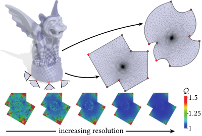
(See examples in Figure 1.) The target shape can be efficiently updated via backsubstitution, providing a new paradigm for conformal parameterization: rather than waiting for a single, predetermined flattening, one can interactively edit or optimize the map—even on meshes with hundreds of thousands of elements. More broadly, BFF is a drop-in replacement for widely-used schemes like least-squares conformal maps (LSCM) while providing sophisticated control over features like shape and area distortion.
1.1. Algorithm Outline
Given a target length (or curvature) function along the boundary, the BFF algorithm involves three basic steps:
- I.
Solve for a compatible curvature (or length) function.
- II.
Integrate this data to get a boundary curve.
- III.
Extend this curve over the interior of the domain.
Computation amounts to solving three sparse linear problems (in steps I and III) connected by a simple nonlinear change of variables (step II); all linear problems use the same fixed Laplace matrix. From here, the essential question is how to devise boundary data (curvatures or lengths) suitable for a variety of mapping problems, as explored in Sec. 6. An important limitation of BFF is that it applies only to domains with disk topology, though of course a surface of any topology can be cut into one or more disks; see Sec. 7.5 for further discussion. Detailed pseudocode is provided in App. B.
2. Related Work
The literature on surface flattening and computational conformal geometry is vast [Sheffer et al., 2006; Gu and Yau, 2008]—here we focus on conformal flattening methods that provide control over boundary shape, or that can be modified to provide such control. Early methods for conformal flattening compute a piecewise linear least-squares solution of the Cauchy-Riemann equations (LSCM [Lévy et al., 2002]), or equivalently, minimize the difference between Dirichlet energy and the flattened area (DCP [Desbrun et al., 2002]); quality was later improved via a sparse eigenvalue problem (SCP [Mullen et al., 2008]). A different line of methods directly optimizes angles in the flattened mesh to approximate angles in the input [Sheffer and de Sturler, 2001; Sheffer et al., 2005], a process that can be linearized without compromising quality (LinABF [Zayer et al., 2007]).
![[Uncaptioned image]](1704.06873v2/Family.png)
Free Boundary Conditions.
The methods mentioned so far forgo the question of boundary control, instead opting for so-called “free” boundary conditions where a discrete energy is minimized without explicit constraints on boundary degrees of freedom. Although this approach provides a unique solution in the discrete setting, it has no meaningful interpretation in the smooth setting: in the absence of explicit boundary conditions there is an enormous space of perfect conformal flattenings, obtained by flattening and then applying an in-plane conformal map (see inset). The only possibility is that the unique solution chosen by free boundary methods must depend on discretization, meaning that results will change depending on the particular choice of mesh or numerical treatment (see Figure 2, and Mullen et al. [2008, Figure 1]). This phenomenon further motivates the need for more careful treatment of boundary conditions.

Prescribed Boundary Length/Angle.
Later methods explicitly incorporate boundary constraints. For instance, the method of circle patterns (CP [Kharevych et al., 2006]) provides control over the direction of the boundary (but not its length); methods based on discrete Ricci flow [Luo, 2004; Jin et al., 2008] can provide control over both length and direction (CETM [Springborn et al., 2008]). All of these methods demand nonlinear optimization involving, e.g., repeated matrix factorization for each Newton iteration. In Sec. 7.1 we explore how linearization of both angle-based (LinABF) and length-based strategies (CPMS [Ben-Chen et al., 2008]) can be adapted to provide complete boundary control; even then, these methods remain at least 30x slower than BFF and can exhibit significant artifacts. A very different approach is to discretize a time-independent Dirac equation that governs conformal surface deformations in 3D [Crane, 2013, Section 6.1]; this approach provides control over boundary direction (but not length) and must solve an eigenvalue problem that cannot be prefactored for varying boundary data.
Uniformization.
A natural idea for achieving a given target shape is to compose maps to a canonical domain like the circular disk (Sec. 6.5). In the discrete setting, however, piecewise linear conformal maps do not compose; more importantly, methods for computing such maps [Zeng et al., 2008; Bobenko et al., 2010] are already more expensive than just directly editing the boundary via BFF.
2D Shape Editing.
Methods for planar shape deformation are generally not suitable for conformal flattening since they depend on boundary element methods or closed-form expressions that are available only on planar domains [Weber and Gotsman, 2010; Lipman et al., 2012; Chen et al., 2013]. One idea is to apply 2D deformation to an initial flattening, but the resulting nonlinear map may be incompatible with the standard geometry processing pipeline, especially when one requires precise control over individual lengths and angles (Sec. 6). Moreover, a composition of methods offers no clear advantage in terms of speed or simplicity over the unified scheme we propose here.
Outside of strictly conformal methods a variety of algorithms provide boundary control, albeit with very different performance characteristics—see for example Weber & Zorin [2014] and references therein. At a high level, all previous boundary-controlled conformal methods (namely, CP and CETM plus our modifications of CPMS and LinABF) indirectly encode a flattening via metric data (lengths or angles). In order for this data to describe a valid planar triangulation it must satisfy nonlinear integrability conditions over the entire domain. In contrast, BFF requires only that data describes a closed boundary curve—a condition that is far easier to satisfy, once the associated integrability conditions are clearly understood.
3. Background
We first provide some key definitions from (discrete) differential geometry; a more pedagogical introduction can be found in Crane et al. [2013] (esp. Chapter 7). Throughout the document, clicking on most symbols will provide a hyperlink back to their definition.
3.1. Notation
Single brackets denote the norm and real inner product ⟨⋅,⋅⟩ of finite-dimensional vectors. For any complex number , and denote the real and imaginary parts, and the imaginary unit ı denotes a quarter-turn in the counter-clockwise direction (hence ). The argument of a complex number is the smallest (in magnitude) signed angle from the real axis to ; the angle from to can therefore be expressed as . Italic glyphs () typically indicate a continuous quantity whereas sans-serif characters () denote discrete quantities and/or matrices.
3.2. Smooth Setting
Our main object of study is a map from a disk-like surface M (with Riemannian metric) to the flat complex plane (Figure 3). At each point the map J rotates any tangent vector by a quarter-turn in the counter-clockwise direction so that (like the imaginary unit) . The boundary ∂M is a single closed loop parameterized by a curve γ with arc-length parameter s. We likewise use to parameterize the image of the boundary ; it is the shape of this curve that we seek to control. By convention, if T is the unit tangent in the direction , then is the outward unit normal. We use K to denote the Gaussian curvature of M, and for the (geodesic) curvatures of γ and ~ γ , respectively.
3.2.1. Conformal Maps
Intuitively, a map is conformal if at each point it preserves the angle between any two vectors, permitting only a uniform change in length. More precisely, let d f denote the differential of f, which determines how a given tangent vector on the surface gets mapped to a tangent vector in the complex plane (in coordinates, d f is represented by the familiar Jacobian matrix). A map f is holomorphic if
| (1) |
for all tangent vectors , i.e., if a quarter-turn J on the surface yields the same result as a quarter-turn ı in the plane; this relationship is known as the Cauchy-Riemann equation. If in addition d f is nondegenerate (i.e., it maps nonzero vectors to nonzero vectors) then f is conformal. The conformal (scale) factor quantifies the change in length at each point (which is independent of direction ); the function is called the log conformal factor.
Conformal maps can also be expressed as pairs of conjugate harmonic functions. A real function is harmonic if it solves the Laplace equation (Sec. 4.1), where Δ is the Laplace-Beltrami operator (or just Laplacian) associated with the domain M. Suppose we express a holomorphic map as for a pair of coordinate functions . Then (by Cauchy-Riemann)
| (2) |
i.e., the gradients of the two coordinates are orthogonal and have equal magnitude. Since a quarter-rotation of a gradient field is divergence-free, we have
and similarly, . In other words, the two real components of a holomorphic function are both harmonic—we say that and form a conjugate harmonic pair.

To what degree can one control the target shape of a conformal flattening? Equation 2 suggests there must be some limitation, since two arbitrary functions on the boundary may not extend to a conjugate harmonic pair on the interior. And yet the Riemann mapping theorem states that any disk-like region can be conformally mapped to the unit circular disk (Sec. 6.5); hence any shape can be obtained via composition with an (inverse) Riemann map. These two facts do not contradict each-other: although one can surjectively map onto any given region (), one cannot arbitrarily “pin” each boundary point to a specific location () and hope to remain conformal. We therefore express our basic algorithm in terms of geometric quantities that can always be realized: one can specify either length or curvature density along the boundary, but not both simultaneously (see Figure 4, Sec. 4.2 and [Springborn et al., 2008, Section 4]). This data can then be further manipulated to provide a variety of intuitive control schemes (Sec. 6).
3.2.2. Curvature Density
In developing boundary conditions it helps to distinguish between the usual pointwise curvatures κ, K, and the corresponding curvature densities, because of the way these quantities transform under a conformal map. Loosely speaking, a density assigns a positive volume to each little piece of a curve or surface, e.g., the length density ds on a curve or the area density dA on a surface. Under a conformal map, new and old densities scale according to the conformal factor: and . A curvature density multiples a density by a curvature function—in particular, κds is the (geodesic) curvature density of a curve, and KdA is the Gauss curvature density of a surface. The change of curvature density under a conformal map is studied in Sec. 4.2.
3.3. Discrete Setting
We discretize our surface as a manifold triangle mesh with disk topology, using to denote the set of vertices on the boundary ∂M, and for interior vertices. Tuples of vertex indices are used to specify simplices, e.g., is an edge from vertex to vertex . An expression of the form means that a quantity is summed over all edges containing vertex to get the value of at . Likewise, denotes a sum over faces containing vertex . A quantity at corner of triangle is denoted by a subscript and superscript ; for instance, we use to denote the interior angle at the corner of a triangle. Throughout we use to denote the dual cell associated with vertex , and to denote the barycentric dual edge associated with a boundary vertex ; denotes the unit tangent along boundary edge (see inset). We use ℓ i j to denote the length of edge in the input mesh, and to denote the length of the dual boundary edge , where , , and are consecutive vertices along the boundary.
3.3.1. Discrete Curvature
Gaussian curvature.
For each interior vertex of a triangulation the angle defect quantifies the “flatness” of a vertex as a deviation from the planar angle sum of . This quantity encodes not the pointwise Gaussian curvature, but rather the curvature integrated over a small region around the vertex: (since for a discrete surface is a distribution concentrated at vertices). We therefore refer to Ω as a discrete curvature density.
Geodesic curvature.
At boundary vertices, the Gaussian curvature (density) is zero, since a small neighborhood around any boundary vertex can be flattened into the plane without stretching. Here we consider a different quantity , which encodes the integral of the geodesic curvature κ (again a distribution at vertices). In the plane, are also the exterior angles, i.e., the change in tangent direction from one edge to the next.
The discrete setting helps illustrate the challenge of prescribing pointwise curvature rather than curvature density. Suppose we want to achieve a boundary curvature κ. If we provide only exterior angles k, then there are in general many polygons that agree with this data (see inset). To uniquely prescribe a target shape, we must be able to control the change in angle per unit length. Likewise, to prescribe Gaussian curvature, we must be able to control the angle defect per unit area. Algorithmically this goal is difficult to achieve since the final lengths and areas are are determined by a scale factor u that is not known a priori—any algorithm that prescribes angle defects (such as CPMS or CETM) actually controls the (discrete) curvature density rather than the curvature itself. One approach to this problem is described in Sec. 6.6.
4. Toolbox
We first describe a collection of basic building blocks, which are assembled into the final algorithm in Sec. 5.
4.1. Poisson Problems
The development of BFF hinges on careful treatment of boundary conditions for the Dirichlet-Poisson problem
| (3) |
and the Neumann-Poisson problem
| (4) |
where a and ϕ are real-valued functions on M, and determine the values or normal derivatives along the boundary, resp. The solution to Eqn. 4 is unique only up to a constant, which in BFF just determines the global scale and translation. On a triangle mesh, integrating over dual cells yields a matrix equation
where is the so-called cotan-Laplace matrix since its nonzero entries can be expressed as
for each edge with opposite vertices , and for each vertex (see Crane et al. [2013, Section 6.3] for a derivation); omitting the unknown cotans at boundary edges corresponds to zero-Neumann boundary conditions (MacNeal [1949, Eqn. 3.3]). The matrix is the mass matrix, but is not needed for BFF since all values appearing on the right-hand side will be integrated quantities (e.g., the discrete Gaussian curvature Ω).
If we partition into interior vertices I and boundary vertices B, a Neumann-Poisson problem can be expressed in block form as
| (5) |
where is the discrete Neumann boundary data, corresponding to the integral of over each dual boundary edge . A Dirichlet problem with boundary values is then obtained by solving the first row of Eqn. 5 for the interior values :
| (6) |
Efficient Solution
Solving a sequence of Dirichlet- and Neumann-Poisson problems requires only a single sparse Cholesky factorization of the matrix A from the Neumann problem. To see why, consider the blockwise expansion
| (7) |
which means the Cholesky factorization for the Dirichlet problem is already given by the upper-left block: . All subsequent problems can then be solved (via backsubstitution) at a small fraction of the factorization cost—since BFF solves only Poisson problems, the computational bottleneck is the single factorization of A. (In practice one needs to be careful about reordering; see Sec. 7.4 for details.) Note that no corresponding treatment is known for LSCM/SCP despite repeated A blocks—the closest proposal entails either dense factorization, or else iterative solvers with no amortized gains from prefactorization [Alexa and Wardetzky, 2011, Section 5.2].
4.2. Cherrier Formula
The change in curvature under a conformal mapping has a close relationship with the scale factor u. For domains without boundary this relationship is captured by the Yamabe problem [Aubin, 1998, Chapter 5], but our method depends critically on additional boundary conditions studied by Pascal Cherrier [1984]. In particular, for a conformal map between any two surfaces,
| (8) |
where Δ is the Laplacian on M, and are the new curvatures on . Although the equation is standard, its boundary conditions have been largely neglected by conformal flattening algorithms, which instead optimize discrete variables without reference to an underlying continuous equation [Kharevych et al., 2006; Springborn et al., 2008], or consider only the special case where ~ κ is a delta distribution [Bunin, 2008; Myles and Zorin, 2013]. We address the general case by multiplying Eqn. 8 through by dA and ds (resp.) to obtain a linear relationship between densities:
| (9) |
| (10) |
Integrating Eqn. 9 over dual cells hence yields a linear relationship
| (11) |
where are the source and target angle defects (see Sections 3.3.1 and 4.1); for flattening, . Likewise, integrating Eqn. 10 over dual boundary edges yields the linear equation
| (12) |
where h is the discrete Neumann data, and are discrete boundary curvatures on the domain and target. Note that (as discussed in Ben-Chen et al. [2008, Section 2.3]) one does not obtain exact target curvatures if u values are used to rescale edge lengths (à la CETM); in BFF we take an alternate route where angles are obtained directly from the discrete Cherrier formula, and exactly satisfy necessary conditions for closure of the target boundary loop (Proposition 1) and realization of target cone angles (Proposition 2).
4.3. Poincaré-Steklov Operators
A given solution to an elliptic boundary value problem (like Poisson) can often be explained by several different types of boundary conditions—for instance, a harmonic function is uniquely determined by either its values (Dirichlet) or normal derivatives (Neumann) along the boundary. In general, a Poincaré-Steklov operator maps boundary data from one solution to alternative boundary data that yields an identical solution. We require two such operators: the Dirichlet-to-Neumann map for a Poisson equation, and the Hilbert transform for the Cauchy-Riemann equation.
4.3.1. Dirichlet to Neumann

Given Dirichlet boundary values g for a discrete Poisson equation, we seek Neumann values h that yield the same solution. One idea is to simply solve the Dirichlet problem, then evaluate the normal derivative directly—e.g., dot unit normals with the solution gradient, then integrate over dual boundary edges . In practice, however, this approach yields poor behavior (see Figure 5, center). A more principled approach is to solve for Neumann data h that exactly reproduces the discrete Dirichlet solution. For a Laplace problem (i.e., ) solving Equations 5 and 6 for h entails evaluating the so-called Schur complement of A:
| (13) |
For a Poisson equation with nonzero source term ϕ, the Dirichlet-to-Neumann map becomes an affine operator given by the expression
| (14) |
In practice this map can be evaluted via a single linear solve involving the (prefactored) matrix together with a sequence of basic matrix operations, as detailed in Alg. 3. In effect, solves a Dirichlet-Poisson equation, then takes the difference between the source term ϕ and the Laplacian of the Poisson solution at each boundary node. Beyond improved numerical behavior (Figure 5, right), this discretization provides a useful invariant in the context of conformal flattening: discrete curvatures k computed via Eqn. 12 always sum to exactly (App. A), automatically satisfying a necessary condition for integrability (Sec. 4.5).
4.3.2. Neumann to Dirichlet
4.3.3. Hilbert Transform
On a disk-like domain, the Hilbert transform H maps the tangential derivative of a harmonic function a to the normal derivative of its harmonic conjugate b, providing boundary data for a holomorphic function (Sec. 3.2.1). Notions of conjugacy have been studied for a wide variety of discretizations [Polthier, 2000; Mercat, 2001; Weber and Gotsman, 2010; Bobenko and Günther, 2015]; in our context, we seek a pair of standard piecewise linear functions with degrees of freedom at vertices. The basic idea is to fix a and solve for the function b that minimizes the least-squares conformal energy E C , which measures the failure of f to satisfy Cauchy-Riemann [Lévy et al., 2002]. This energy can also be expressed as the Dirichlet energy of f minus the area of its image [Hutchinson, 1991], which in matrix form becomes
| (15) |
where encodes the signed area of the boundary polygon:
| (16) |
(see [Mullen et al., 2008, Section 2.2]). Minimizing E C with fixed a therefore amounts to solving the Neumann-Laplace equation . The Neumann boundary data can be obtained by differentiating Eqn. 16 with respect to b, yielding the simple expression
| (17) |
for any three consecutive vertices along the boundary. Notably, this expression looks like a naïve finite difference—the variational interpretation above verifies that it nonetheless yields a solution that is “as conjugate as possible” in the least-squares sense.
4.4. Interpolation
Suppose we want to extend a given function over the interior of the domain, i.e., find a map such that . A simple strategy is to independently interpolate each coordinate of ~ γ by a harmonic function, i.e., solve a pair of Laplace problems
If ~ γ is already compatible with some holomorphic map f, the Hilbert transform H from the previous section provides a different strategy:
- (1)
(Harmonic extension.) Solve s.t. .
- (2)
(Harmonic conjugation.) Solve s.t. ,
where the discrete Neumann data for the latter problem is computed via Eqn. 17. These two strategies provide different algorithmic invariants: with the former, f exactly interpolates ~ γ but is not guaranteed to be exactly holomorphic; with the latter f is holomorphic but may not exactly interpolate both components of ~ γ . When ~ γ comes from a holomorphic map they will coincide; in practice, each is best-suited to different applications, as discussed in Sec. 6.
4.5. Curve Integration
A key step in BFF is recovering a closed boundary curve ~ γ from given curvature and length data. In the smooth setting this data can be integrated directly, but in the discrete case a small amount of discretization error prevents closure—we therefore seek a closed curve that approximates the given data. Directly optimizing vertex positions leads to a difficult nonlinear problem; we instead solve an easy convex problem that closes the curve by minimally adjusting length. In the smooth setting, we formulate this problem by considering the cumulative curvature
We then construct unit tangents along the boundary and solve the problem
| (18) |
If κ already describes a closed loop then we recover the solution ; otherwise, r minimally adjusts the speed of the curve such that it closes. In either case, we obtain the final curve by integrating the scaled tangents:
4.5.1. Discretization
To discretize Eqn. 18, let specify the desired exterior angles and edge lengths (Figure 6, right). We seek a polygon with vertices that exactly achieves these angles and closely matches the lengths. We first compute cumulative angles
and target tangents . Eqn. 18 then becomes
| (19) |
If is a diagonal mass matrix with entries and we pack the two coordinates of each unit tangent into a matrix , then the optimal lengths are given by
| (20) |
Note that is just a matrix which costs virtually nothing to build and invert. Final vertex positions are recovered via the cumulative sums In principle the new lengths ~ ℓ i j could become negative, but in practice we do not observe this behavior: typical values for are in the range .
5. Algorithm
We now describe the basic boundary first flattening algorithm using tools from Sec. 4, as summarized in Figure 7.
Input. A triangle mesh with disk topology and either (i) desired scale factors u or (ii) target exterior angles ~ k at boundary vertices. In the latter case, angles must sum to .
Output. A piecewise linear map which approximates a smooth conformal map with the given boundary data (u or ~ k ).
Algorithm.
Step I uses the Cherrier formula to “explain” the provided boundary data: if scale factors were given, what must the curvature look like under a conformal flattening (and vice versa)? The map (or ) is used to evaluate this formula; using a source term Ω corresponds to setting the target Gaussian curvature to , i.e., flattening. Since the resulting boundary data is compatible with some conformal flattening, the exterior angles ~ k and scaled boundary lengths ℓ ∗ already describe a valid closed loop—modulo a small amount of discretization error which is accounted for by the integration procedure in Step II. (Here we scale ℓ by the mean conformal factor à la CETM, though any consistent approximation will work.) Since length adjustments during integration are very small, the resulting curve ~ γ remains extremely close to the boundary of some conformal map. Therefore, in Step III a holomorphic extension of either coordinate function or will yield an accurate approximation of a conformal map that closely matches the input data—as verified by numerical experiments in Sections 6 and 7.
The overall cost is one factorization of a real cotan-Laplace matrix, followed by three backsolves: one to evaluate the map Λ or in Step I; two to compute the holomorphic extension in Step III. All other operations require only work, involving simple closed-form expressions evaluated at boundary vertices. (See Sec. 7 for detailed performance analysis.)
6. Applications
We now use the core BFF algorithm to solve several problems in surface parameterization. The basic question is how to construct appropriate boundary data (scale factors or curvatures) for each task.
6.1. Automatic Parameterization
In the absence of user-specified criteria, a natural choice of conformal flattening is the one with minimal area distortion. Springborn et al. [2008, App. E] show that such a map is obtained by prescribing zero scale factors along the boundary (). Figures 1, 2, and 14 show results computed via BFF, which are virtually indistinguishable from those produced by CETM (albeit at far lower cost) and respect features like symmetry even better than SCP (Figure 2). These boundary conditions provide the baseline for later comparisons with existing automatic methods (Sec. 7).
6.2. Direct Editing
A natural way to edit conformal flattenings with BFF is to directly manipulate the angles (relative to the real axis) or length ℓ ∗ of target edges . These values can then be easily converted to curvatures ~ k and scale factors u per boundary vertex (resp.). In particular the (integrated) curvatures are simply
Converting target lengths ℓ ∗ i j (per boundary edge) to target scale factors (per boundary vertex) is more subtle. One idea is to solve the linear system for scale factors u that satisfy discrete conformal equivalence [Springborn et al., 2008]. However, this system does not always have a solution; hence, even metric-based methods like CETM and CMPS cannot (in general) exactly prescribe boundary lengths. We instead use a straightforward numerical approximation: compute scale factors per boundary edge, then integrate over dual boundary edges to get
where , , and are consecutive vertices along the boundary.
As an experiment, we use a spline-based curve editor to nonrigidly pack surface charts into a texture atlas (Figure 8). At each vertex, boundary values are sampled from a real-valued Catmull-Rom spline (and normalized to in the case of curvatures). The Dirichlet-to-Neumann map Λ is applied to the current boundary data to switch between angle- and length-based editing.

6.3. Sharp Corners
![[Uncaptioned image]](1704.06873v2/RoundRectRefinement.png)
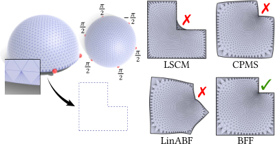
For target shapes with sharp corners (like a rectangle) the standard BFF procedure can exhibit undesirable rounding (see inset, top). Here we can replace the holomorphic extension in Step III with a simple harmonic extension (Sec. 4.4), thereby interpolating the polygon ~ γ reconstructed in Step II, and exactly reproducing the requested angles. Since ~ γ approximates the boundary of a conformal map, both procedures still converge to a holomorphic function under refinement (see inset and Figure 9, bottom). Simpler algorithms for mapping to polygons can only handle special cases like rectangles [Zeng et al., 2008, Section 4.1] or are limited to straight edges [Driscoll and Trefethen, 2002]; compare with the piecewise curved boundary in Figure 9, top right. Note that with piecewise linear maps it is impossible for any algorithm to completely eliminate angle distortion near corners, since the initial and target angle sums will differ even under refinement.
6.4. Cone Parameterization

A powerful technique for mitigating area distortion (Figure 10) is to first map to a cone surface, which is flat () away from a collection of isolated cone points [Kharevych et al., 2006]. After cutting through these points, it can be flattened into the plane without further distortion (Figure 10, right). A variety of strategies are available for picking cones [Kharevych et al., 2006; Ben-Chen et al., 2008; Springborn et al., 2008]; we assume they have been specified by the user as target curvatures per interior vertex (mostly zero). For a closed surface of genus , Θ must sum to , by Gauss-Bonnet. To compute a cone flattening of an initial surface , we:
- (1)
Solve the Cherrier problem for u, with source term .
- (2)
Cut into a disk M via a cut passing through all cones.
- (3)
Apply Alg. 1, prescribing u values from Step 1 along .
Springborn et al. [2008, Section 3.3] describe one possible cutting procedure. To obtain a seamless map, we associate only a single length degree of freedom ~ ℓ with each pair of corresponding cut edges in Eqn. 18; angles are automatically complementary, by Proposition 2, and a harmonic extension (à laSec. 6.3) ensures this data is exactly preserved in the final layout. The resulting maps are nearly identical to those produced by CETM (Figure 11), though we do not exactly preserve length cross ratios. Unlike CPMS/CETM we never compute (nor need to enforce integrability of) rescaled edge lengths, and can edit cone angles without performing additional factorization; unlike CPMS we guarantee by construction that the map is seamless. Moreover, since the Laplace matrix is modified only along the cut, fast updates of cone locations might also be achieved via low rank updates—see for example Essid & Solomon [2017].

6.5. Uniformization
A popular use of conformal maps is to provide a common reference domain for comparative data analysis [Lipman and Daubechies, 2011; Koehl and Hass, 2015]. For surfaces with disk topology, the uniformization theorem guarantees the existence of conformal maps to the unit circular disk—any such map has constant boundary curvature . However, prescribing a constant curvature density yields a shape that is merely convex rather than circular. Instead, we use a simple fixed-point scheme: if the target curvature ~ κ were equal to 1, then the target curvature density would be , i.e., just the new length density. Hence, at the th iteration we prescribe target angles proportional to the most recent dual edge lengths:
We then compute a conformal flattening and repeat. To stabilize this process we average with the previous guess (i.e., ), using the discrete geodesic curvatures of the input surface as our initial guess. We also find that a harmonic rather than holomorphic extension (Sec. 6.3) yields better results, especially for domains with jagged boundaries. In practice we always converge in about 10 iterations—since each iteration involves only backsubstitution the total cost is similar to a single LSCM solve, but produces results nearly identical to nonlinear methods (as depicted in Figure 12). A canonical map can be found by picking the Möbius transformation that best balances area distortion, à la [Springborn, 2005].
6.6. Arbitrary Curves
We can map a surface to an arbitrary target shape using a similar strategy: since a plane curve is determined by its curvature (up to rigid motion), we iteratively prescribe the curvature density , where is our most recent guess for the scale factor. In the discrete case, let be a desired closed, arc-length parameterized curve; let be the cumulative sum of boundary edge lengths at the current iteration, and let be the total length. We first sample to obtain a polygon with vertices , i.e., at intervals proportional to our most recent edge lengths. We then compute the exterior angles of the sampled curve . Since the sample points are determined using the most recent length density, these angles provide an estimate for the desired curvature density. Empirically, this procedure rapidly converges to the target shape (see Figure 13). Basic as this functionality may seem, it is not provided by any previous conformal flattening algorithm (linear or nonlinear)—the closest comparison is the recent method of Segall and Ben-Chen [2016] for in-plane conformal deformations.
7. Evaluation and Comparisons


Here we consider the numerical quality and runtime performance of both linear and nonlinear methods for boundary-controlled conformal flattening, including modifications of existing linear schemes. To help avoid erroneous comparisons, LSCM, SCP, LinABF, CP, CPMS, and CETM were independently implemented by both authors, and compared with reference implementations wherever possible. Figure 14 confirms that all implementations of boundary-controlled methods produce similar results (albeit at very different costs).
7.1. Modified Linear Methods
Though previous linear conformal flattening methods do not explicitly address boundary control, it is natural to ask whether we simply need to modify their boundary conditions. Below we explore such modifications for two linear methods (CPMS and LinABF).
7.2. Boundary-Controlled CPMS
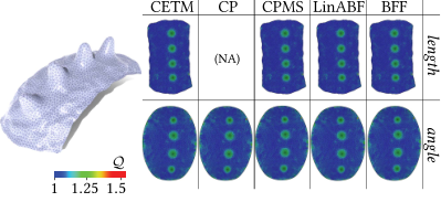
Like BFF, CPMS [Ben-Chen et al., 2008] employs a Yamabe-type equation (Sec. 4.2) to obtain scale information. There are however several key differences. First, CPMS does not provide direct control over boundary shape: boundary vertices “absorb” curvature via a process that entails a Poisson solve per boundary vertex—even with prefactorization these solves become quite expensive (Ben-Chen et al. [2008, Section 4.2]). Second, it uses a different layout strategy: whereas BFF need only ensure that boundary data describes a closed loop (Sec. 4.5), CPMS seeks edge lengths that describe a closed, flat surface. Rather than satisfy this condition exactly (à la CETM), best-fit vertex positions are found via a least-squares problem [Sheffer et al., 2005] which cannot be prefactored since the matrix itself depends on the augmented lengths. We can of course add boundary control by incorporating Eqn. 8: to control angles we apply the Dirichlet-to-Neumann map (as in Step I of BFF); to control length we simply set Dirichlet boundary values for u. For nice meshes and smooth boundary data this strategy works well (Figure 14) but in general may exhibit artifacts since the least-squares layout does not respect boundary constraints (Figure 15). The amortized cost of editing a map via BFF remains about 30x faster than CPMS with our boundary modification, or about 50x faster than the original method (due to numerous solves at boundary vertices)—see Figure 17.
7.3. Boundary-Controlled LinABF
In angle-based flattening (ABF) [Sheffer and de Sturler, 2001] a near-flat metric is found by optimizing corner angles β; a least-squares layout then provides planar vertex positions approximating these angles. Zayer et al. [2007] linearize ABF, solving for angle adjustments relative to an initial guess —this strategy yields results nearly identical to the original algorithm. We modify this approach in two ways. First, to prescribe exterior angles ~ κ we simply add linear constraints at each boundary vertex . Second, to prescribe boundary lengths ~ ℓ i j (up to global scale) we incorporate the condition
for each boundary vertex, i.e., we use the law of sines to prescribe the ratio of consecutive edge lengths along the boundary (see inset). Taking the first-order approximation of the logarithm and substituting for in the final system (à la Zayer) then yields linear constraints. As with CPMS, this strategy works well for nice meshes (Figure 14) but can produce artifacts due to both linearization and the least-squares layout (Figure 15). Moreover, neither the least-squares matrix nor the larger angle constraint matrix can be prefactored, yielding lower performance than other linear methods (Figure 17).

7.4. Quality and Performance
We measure angle distortion via quasi-conformal error , which is the ratio of singular values of the mapping in each face [Sander et al., 2001]; is ideal, and denotes the area weighted average over the surface. Area distortion is measured via the log scale factor u, which is shifted to have zero mean.
Single-threaded performance was measured on a 3.3GHz Intel Core i7 with 16GB of memory. All methods were implemented in C++ using double precision. Linear methods use the supernodal factorization in CHOLMOD [Chen et al., 2008]. To extract the subfactor (Sec. 4.1) we compute a block-preserving reordering via cholmod_l_camd, which has no impact on factorization cost or factor density; overall we achieve a real-world 2x speedup over computing separate Neumann and Dirichlet factors. For CP we used MOSEK [ApS, 2010]. For CETM we used Newton’s method with backtracking line search [Boyd and Vandenberghe, 2004, Algorithms 9.2 and 9.5], which in our tests performed better than L-BFGS or Newton trust region; during editing, using a previous solution as an initial guess did not significantly reduce the number of Newton iterations (especially for large changes to boundary data).
Figure 16 suggests that our proposed strategy converges to a perfectly conformal map under refinement at the same (linear) rate as all other flattening methods. Figure 17 verifies that real-world timings agree with expected bottlenecks based on the size and number of matrices that must be factored [Botsch et al., 2005]. (Here LSCM/SCP/CPMS/CP use free boundary conditions; all other methods set .) The takeaway from these experiments is not that any method provides a big win in terms of accuracy (note the narrow vertical range in Figure 17) but simply that BFF does not sacrifice quality for speed. In particular, by using prefactorization BFF enables conformal flattenings to be edited about 30x quicker than the next-fastest boundary-controlled method (Modified CPMS), and about 50x quicker than the fastest previously-published method (CETM). This level of improvement provides a qualitative shift in the type of applications that can afford to use sophisticated conformal flattening—e.g., interactive applications, or optimization for computational design [Konakovic et al., 2016].
7.5. Guarantees and Limitations
Boundary Data.
Two guarantees provided by BFF are (i) exact realization of prescribed angles when using harmonic extension (as discussed in Sec. 6.3) and (ii) exact compatibility of lengths and angles along cuts (as discussed in Sec. 6.4). Neither LinABF nor CPMS can provide such guarantees since the least-squares layout step ignores any prescribed boundary data. Both CP and CETM will exactly satisfy angle constraints so long as optimization converges to an accurate solution. Exact length constraints are difficult for all methods, as discussed in Sec. 6.2.
Injectivity.
A result of Floater [2003, Theorem 4.1] implies that maps produced by BFF are locally injective as long as (i) prescribed angles k are positive (describing a convex target), (ii) the discrete Laplacian A exhibits a maximum principle, and (iii) adjusted edge lengths ~ ℓ are positive. The Delaunay condition is sufficient (but not necessary) to ensure condition (ii); length adjustments are typically miniscule and hence far from negative (Sec. 4.5.1).
![[Uncaptioned image]](1704.06873v2/FlippedTriangle.png)
In practice we find that flips are quite rare: for instance, 6 of 588 meshes in the SHREC 2011 database had one or two flipped triangles, with a total flipped area on the order of when normalized to unit radius (see inset); for each mesh we automatically placed eight cones à la Ben-Chen et al. [2008]. Often such flips are easy to fix; one could also perform local Delaunay remeshing, or fall back to a more expensive injective method (see references in [Smith and Schaefer, 2015]), though such methods may not provide the desired boundary control.

Topology.
For topological spheres one can remove a single vertex star and map to the circular disk, then to the unit sphere via stereographic projection. For multiply-connected domains like the annulus, the Cherrier formula (Eqn. 8) is still valid but describes only an intrinsic flattening that may not admit a planar layout (consider cutting the tip from a circular cone); moreover, the Hilbert transform (Sec. 4.3.3) is valid only for disk-like domains. In practice, of course, BFF can be used to flatten any surface by cutting it into one or more disks (Figs. 18, 8, and 10).
Target Geometry.
BFF provides flattening only over Euclidean domains (possibly with cone singularities), unlike methods based on discrete Ricci flow [Jin et al., 2008; Springborn et al., 2008] which can target spherical or hyperbolic geometry. However, since the Cherrier formula is valid for any target curvature it would be interesting to generalize the boundary-first strategy—here one might apply an iterative strategy akin to Sec. 6.5 to prescribe pointwise Gaussian curvature (rather than Gaussian curvature density).
8. Acknowledgements
Thanks to Tim Davis for help with block reordering and supernodal subfactor extraction in CHOLMOD. This work was funded in part by a gift from Autodesk, Inc.
References
- Alexa and Wardetzky [2011] Marc Alexa and Max Wardetzky. 2011. Discrete Laplacians on General Polygonal Meshes. ACM Trans. Graph. 30, 4 (2011).
- Alliez et al. [2003] Pierre Alliez, Éric Colin de Verdière, Olivier Devillers, and Martin Isenburg. 2003. Isotropic Surface Remeshing. In Proc. Shape Modeling International.
- ApS [2010] Mosek ApS. 2010. The MOSEK optimization software. http://www.mosek.com (2010).
- Aubin [1998] T. Aubin. 1998. Some Nonlinear Problems in Riemannian Geometry. Springer Berlin.
- Ben-Chen et al. [2008] Mirela Ben-Chen, Craig Gotsman, and Guy Bunin. 2008. Conformal Flattening by Curvature Prescription and Metric Scaling. CG Forum (2008).
- Bobenko et al. [2010] A. Bobenko, U. Pinkall, and B. Springborn. 2010. Discrete conformal maps and ideal hyperbolic polyhedra. ArXiv e-prints (2010).
- Bobenko and Günther [2015] A. I. Bobenko and F. Günther. 2015. Discrete complex analysis on planar quad-graphs. ArXiv e-prints (2015).
- Botsch et al. [2005] Mario Botsch, David Bommes, and Leif Kobbelt. 2005. Efficient Linear System Solvers for Mesh Processing. In Proc. IMA Int. Conf. Math. Surf. 62–83.
- Boyd and Vandenberghe [2004] Stephen Boyd and Lieven Vandenberghe. 2004. Convex Optimization. Cambridge University Press.
- Bunin [2008] Guy Bunin. 2008. A continuum theory for unstructured mesh generation in two dimensions. In CAGD, Vol. 25. 14–40.
- Chao et al. [2010] Isaac Chao, Ulrich Pinkall, Patrick Sanan, and Peter Schröder. 2010. A Simple Geometric Model for Elastic Deformations. ACM Trans. Graph. 29, 4 (2010).
- Chen et al. [2013] Renjie Chen, Ofir Weber, Daniel Keren, and Mirela Ben-Chen. 2013. Planar Shape Interpolation with Bounded Distortion. ACM Trans. Graph. 32, 4 (2013).
- Chen et al. [2008] Yanqing Chen, Timothy A. Davis, William W. Hager, and Sivasankaran Rajamanickam. 2008. Algorithm 887: CHOLMOD, Supernodal Sparse Cholesky Factorization and Update/Downdate. ACM Trans. Math. Softw. 35, 3 (2008).
- Cherrier [1984] Pascal Cherrier. 1984. Problèms de Neumann non linéaires sur les variétés riemanniennes. Journal of Functional Analysis 57 (1984), 154–206.
- Crane [2013] Keenan Crane. 2013. Conformal Geometry Processing. Ph.D. Dissertation. Caltech.
- Crane et al. [2013] Keenan Crane, Fernando de Goes, Mathieu Desbrun, and Peter Schröder. 2013. Digital Geometry Processing with Discrete Exterior Calculus. In SIGGRAPH Courses.
- Desbrun et al. [2002] Mathieu Desbrun, Mark Meyer, and Pierre Alliez. 2002. Intrinsic Parameterizations of Surface Meshes. CG Forum (2002).
- Driscoll and Trefethen [2002] T.A. Driscoll and L.N. Trefethen. 2002. Schwarz-Christoffel Mapping. Cambridge University Press.
- Essid and Solomon [2017] Monty Essid and Justin Solomon. 2017. Quadratically-Regularized Optimal Transport on Graphs. (in submission) (2017).
- Floater [2003] Michael S. Floater. 2003. One-to-one piecewise linear mappings over triangulations. Math. Comp. 72 (2003), 685–696.
- Gu and Yau [2008] X.D. Gu and S.T. Yau. 2008. Computational Conformal Geometry. International Press.
- Hurdal and Stephenson [2009] Monica K. Hurdal and Ken Stephenson. 2009. Discrete conformal methods for cortical brain flattening. NeuroImage 45, 1 (2009), 86–98.
- Hutchinson [1991] John E. Hutchinson. 1991. Computing conformal maps and minimal surfaces. In Theoretical and Numerical Aspects of Geometric Variational Problems. 140–161.
- Jin et al. [2008] Miao Jin, Xianfeng Gu, Feng Luo, and Junho Kim. 2008. Discrete Surface Ricci Flow. IEEE Trans. Vis. Comp. Graph. 14 (2008), 1030–1043.
- Kharevych et al. [2006] Liliya Kharevych, Boris Springborn, and Peter Schröder. 2006. Discrete Conformal Mappings via Circle Patterns. ACM Trans. Graph. 25, 2 (2006), 412–438.
- Kim et al. [2012] Jungwook Kim, James A. Hanna, Myunghwan Byun, Christian D. Santangelo, and Ryan C. Hayward. 2012. Designing Responsive Buckled Surfaces by Halftone Gel Lithography. Science 335, 6073 (2012), 1201–1205.
- Koehl and Hass [2015] Patrice Koehl and Joel Hass. 2015. Landmark-free geometric methods in biological shape analysis. Journal of The Royal Society Interface 12, 113 (2015).
- Konakovic et al. [2016] Mina Konakovic, Keenan Crane, Bailin Deng, Sofien Bouaziz, Daniel Piker, and Mark Pauly. 2016. Beyond Developable: Computational Design and Fabrication with Auxetic Materials. ACM Trans. Graph. 35, 4 (2016).
- Lévy et al. [2002] Bruno Lévy, Sylvain Petitjean, Nicolas Ray, and Jérome Maillot. 2002. Least Squares Conformal Maps. ACM Trans. Graph. 21, 3 (2002).
- Lipman and Daubechies [2011] Y. Lipman and I. Daubechies. 2011. Conformal Wasserstein distances: comparing surfaces in polynomial time. ArXiv e-prints (2011).
- Lipman et al. [2012] Yaron Lipman, Vladimir G. Kim, and Thomas A. Funkhouser. 2012. Simple Formulas for Quasiconformal Plane Deformations. ACM Trans. Graph. 31, 5 (2012).
- Liu et al. [2008] Ligang Liu, Lei Zhang, Yin Xu, Craig Gotsman, and Steven Gortler. 2008. A Local/Global Approach to Mesh Parameterization. In Proc. Symp. Geom. Proc. 1495–1504.
- Luo [2004]
Feng Luo. 2004.
Combinatorial
Yamabe Flow on Surfaces.
Comm. Contemp. Math.
/ 06, 05 (2004), 765–780. - MacNeal [1949] Richard MacNeal. 1949. The Solution of Partial Differential Equations by means of Electrical Networks. Ph.D. Dissertation. Caltech.
- Mercat [2001] Christian Mercat. 2001. Discrete Riemann Surfaces and the Ising Model. Comm. Math. Phys. 218, 1 (2001), 177–216.
- Mullen et al. [2008] Patrick Mullen, Yiying Tong, Pierre Alliez, and Mathieu Desbrun. 2008. Spectral Conformal Parameterization. In Proc. Symp. Geom. Proc. 1487–1494.
- Myles and Zorin [2013] Ashish Myles and Denis Zorin. 2013. Controlled-distortion Constrained Global Parametrization. ACM Trans. Graph. 32, 4 (July 2013).
- Polthier [2000] Konrad Polthier. 2000. Conjugate Harmonic Maps and Minimal Surfaces. Preprint No. 446, TU-Berlin, SFB 288 (2000).
- Sander et al. [2001] Pedro V. Sander, John Snyder, Steven J. Gortler, and Hugues Hoppe. 2001. Texture Mapping Progressive Meshes. In Proc. ACM/SIGGRAPH. 409–416.
- Sarkar et al. [2009] Rik Sarkar, Xiaotian Yin, Jie Gao, Feng Luo, and Xianfeng David Gu. 2009. Greedy routing with guaranteed delivery using Ricci flows.. In IPSN. 121–132.
- Segall and Ben-Chen [2016] Aviv Segall and Mirela Ben-Chen. 2016. Iterative Closest Conformal Maps between Planar Domains. CG Forum (2016).
- Segall et al. [2016] Aviv Segall, Orestis Vantzos, and Mirela Ben-Chen. 2016. Hele-Shaw Flow Simulation with Interactive Control. In In Proc. Symp. Comp. Anim. 85–95.
- Sheffer and de Sturler [2001] A. Sheffer and E. de Sturler. 2001. Parameterization of Faceted Surfaces for Meshing using Angle-Based Flattening. Engineering with Computers 17, 3 (2001), 326–337.
- Sheffer et al. [2005] Alla Sheffer, Bruno Lévy, Maxim Mogilnitsky, and Alexander Bogomyakov. 2005. ABF++ : Fast and Robust Angle Based Flattening. ACM Trans. Graph. 24, 2 (2005).
- Sheffer et al. [2006] Alla Sheffer, Emil Praun, and Kenneth Rose. 2006. Mesh Parameterization Methods and Their Applications. Found. Trends. Comput. Graph. Vis. 2, 2 (2006), 105–171.
- Smith and Schaefer [2015] Jason Smith and Scott Schaefer. 2015. Bijective Parameterization with Free Boundaries. ACM Trans. Graph. 34, 4 (July 2015).
- Springborn [2005] Boris Springborn. 2005. A Unique Representation of Polyhedral Types. Centering via Mö̈bius Transformations. Math. Z. 249 (2005), 513–517.
- Springborn et al. [2008] Boris Springborn, Peter Schröder, and Ulrich Pinkall. 2008. Conformal Equivalence of Triangle Meshes. ACM Trans. Graph. 27, 3 (2008).
- Weber and Gotsman [2010] Ofir Weber and Craig Gotsman. 2010. Controllable Conformal Maps for Shape Deformation and Interpolation. ACM Trans. Graph. 29, 4 (2010).
- Weber and Zorin [2014] Ofir Weber and Denis Zorin. 2014. Locally injective parametrization with arbitrary fixed boundaries. ACM Trans. Comp. Sys. 33, 4 (2014).
- Zayer et al. [2007] Rhaleb Zayer, Bruno Lévy, and Hans-Peter Seidel. 2007. Linear Angle Based Parameterization. In Proc. Symp. Geom. Proc. 135–141.
- Zeng et al. [2008] Wei Zeng, Lok Ming Lui, Xianfeng Gu, and Shing-Tung Yau. 2008. Shape Analysis by Conformal Modules. Meth. Appl. Anal. 15, 4 (2008), 539–556.
- Zhong et al. [2014] Zichun Zhong, Liang Shuai, Miao Jin, and Xiaohu Guo. 2014. Anisotropic Surface Meshing with Conformal Embedding. Graph. Models 76, 5 (2014), 468–483.
Appendix A Exact Angle Sums
Proposition 1. For any given scale factors u, the complementary curvatures ~ k computed by Step I of BFF will always sum to exactly .
Proof. Integrating the Cherrier formula over a boundary dual cell yields (since for a flattening). Since at boundary vertices (Sec. 3.3.1), the new boundary curvatures can be expressed as
where is the dual boundary edge at . Their sum is then
where is the union of all interior dual cells (see inset)—note the change in orientation, and cancellation due to equal and opposite normal derivatives in adjacent cells. Applying Gauss-Bonnet to the first term and the divergence theorem to the second, we get
where for a disk . But since (and curvature is nonzero only on ), we are left with just .
Proposition 2. Target angles ~ k computed as in Sec. 6.4 will sum to exactly the desired cone angles Θ.
Proof. Suppose our cut partitions an interior vertex into several regions, and let be the sum of interior angles at in the th region (see inset). Recall that (Eqn. 12), hence
Since ~ k and are supplementary angles, we get
where is the cell boundary on the original (uncut) mesh. Canceling terms and recalling that for our cone parameterization (Sec. 6.4), we get the desired result:
Appendix B Pseudocode
Pseudocode for the basic BFF algorithm (Sec. 5) is included below. Boundary vertices are enumerated by cyclic indices throughout. In lieu of vertex positions, the geometry of the input mesh is specified purely by its edge lengths ℓ, which is useful when the surface is not embedded. In practice, of course, it may be easier to compute quantities like angles directly from vertex positions. For an initial implementation it may be easiest to first separately factor the Dirichlet and Neumann Laplace matrices; extracting a subfactor (à la Eqn. 7) will subsequently improve performance.
All remaining procedures involve either evaluating simple formulas, or calling standard library routines:
- •
— computes the angles at each triangle corner.
- •
— computes discrete Gauss and geodesic curvature using formulas from Sec. 3.3.1. (Note that at all boundary vertices .)
- •
— returns sparse Cholesky factor L.
- •
— solves using the Cholesky factor of .