On the Radio Emitting Particles of the Crab Nebula: Stochastic Acceleration ModelNote: Not to appear in Nonlearned J., 45.

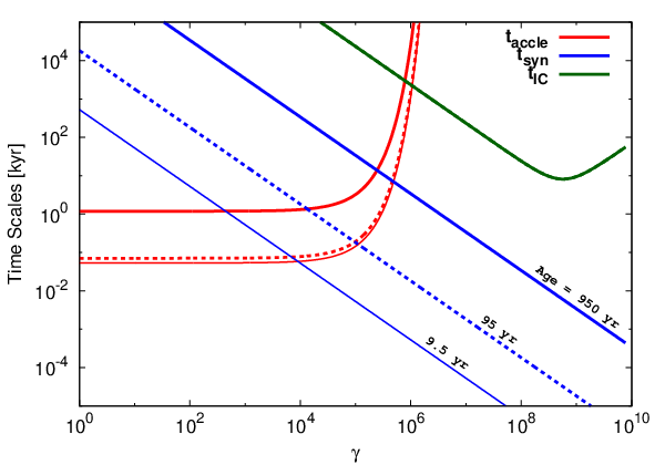
As the first step, we adopt a simple model with the Kolmogorov-like index $q=5/3$, continuous injection ($Q_{\rm ext}=Q_{\rm cont}$), and continuous acceleration ($\tau_{\rm turb}=\infty$, $\gamma_{\rm cut}=\infty$). In addition, here we set the acceleration time-scale as $\tau_{\rm acc,m}=t_{\rm age}$ in order to accelerate the radio-emitting particles from $\gamma_{\rm inj}$ to $\gamma_{\rm min}$ within the age of system. In this case, the parameter to be adjusted is only $\dot{n}_{\rm cont}$. As shown in Figure 1, the parameter value $\dot{n}_{\rm cont}=1.0\times 10^{41}~{\rm s^{-1}}$ marginally reproduce the current broadband spectrum of the Crab Nebula. In this Kolmogorov-like case, the turbulence acceleration hardly affects the evolution of the particles injected above $\gamma_{\rm min}$ (compare the acceleration and cooling time-scales for high energy particles in the bottom-left panel of Figure 1), so that the spectrum of the X-ray-emitting particles almost coincides with the result of TT10. Note that the required small $\eta_{\rm e}\sim 0.35$ compared to TT10 is consistent with the energy budget for the turbulence responsible for the stochastic acceleration (the bottom-right panel of Figure 1). As seen in the top-left panel of Figure 1, the continuously injected particles of $\gamma_{\rm inj}=2$ are stochastically accelerated and forms the radio-emitting particles which have a peak at $\gamma\sim 10^{4}$ at $t=t_{\rm age}$ (thick green). Although the particle spectrum with the two peaks at $t_{\rm age}$ seems significantly different from the result of TT10 (thin black), the broadband emission spectrum seems not far different from the observations (the top-left panel of Figure 1).

The observed spectrum at around $10^{12}-10^{13}$ Hz (we call ‘the infrared bump’ below) contains emission from the dust formed by the SN explosion [75, 53, c.f.,] and then we overlay the 80 $K$ blackbody spectrum in the broadband spectrum just for reference. The emission at the frequencies below the infrared bump is synchrotron emission from the stochastically accelerated particles. We find that the resultant curved spectrum rather than a power-law one does not contradict the flat radio spectrum. The spectral component above the infrared bump to $\sim 10^{23}$ Hz is due to synchrotron emission from the X-ray-emitting particles accelerated at the termination shock $Q_{\rm PSR}$. The $\gamma$-ray emission above $10^{23}$ Hz is mostly from the inverse Compton scattering off the radio synchrotron photons by the X-ray-emitting particles.

In this continuous acceleration model without energy cut off ($\tau_{\rm turb}=\infty$, $\gamma_{\rm cut}=\infty$), the parameter set in Figure 1 is almost the unique one to reproduce the observed broadband spectrum. The energy-dependent acceleration ($q=5/3<2$) and the acceleration time of $\tau_{\rm acc,m}\sim t_{\rm age}$ are required to avoid accelerating particles of $\gamma\geq\gamma_{\rm min}$ in our one-zone treatment. The energy independent acceleration ($q=2$) or shorter acceleration time ($\tau_{\rm acc,m}<t_{\rm age}$) definitely affects the particle spectrum for $\gamma\geq\gamma_{\rm min}$, which leads to a harder X-ray spectrum than observed one. In addition, for $q<2$, the increasing injection rate $s=2$ is essential to form the smooth curved electron spectrum that agrees with the flat radio spectrum. If we adopt $s=0$, the radio spectrum becomes too hard.

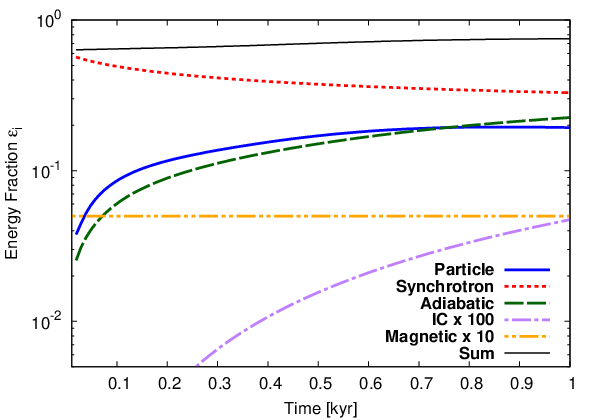
The bottom-right panel of Figure 1 shows evolution of energetics inside the Crab Nebula. The sum of the particle, magnetic, radiated and adiabatically cooled energies (thin black) is about a half of the injected rotational energy $E_{\rm rot}(t)$ and then this is consistent with $\eta_{\rm B}+\eta_{\rm e}\approx 0.35$. The rest of $\sim 0.65E_{\rm rot}(t)$ is interpreted to be stored as the kinetic energy of the turbulent flow and a fraction of it has been used to accelerate the radio-emitting particles already. However, under the assumption of $\tau_{\rm turb}=\infty$, the particle energy (thick blue) keeps increasing and will exceed $E_{\rm rot}(t)$ for $t\gg t_{\rm age}$. A finite value of $\tau_{\rm turb}$ as a feedback process from the particles to the turbulence is required to follow the evolution beyond $t_{\rm age}$.

We have another strong motivation to introduce $\tau_{\rm turb}$. Figure 2 shows the calculated present flux evolution rate with the observations in radio and optical. The current radio observations clearly show that the flux decreases with time, while our continuous acceleration model (dashed green) predicts increase of the radio flux, because the radio-emitting particles are being accelerated even at present. We attempt models with finite $\tau_{\rm turb}$ and $\gamma_{\rm cut}$ to reproduce the flux decrease of the radio emission below. Note that the optical observation would contain potential uncertainty and may not show the secular decrease in contrast to the radio observation [67]. Actually, the X-ray and $\gamma$-ray variabilities are about an order of magnitude larger, and even increasing and decreasing has been observed [89]. Such large variabilities would reflect the contribution from the small emission region close to the termination shock, while the radio flux evolution discussed in Figure 2 is secular evolution of flux from the entire nebula.

Even for a model similar to the simple one in the previous section, a parameter choice of $\tau_{\rm turb}\sim\tau_{\rm acc,m}\sim t_{\rm age}$ may lead to agreement with both the observed spectrum and flux changes, but this accidental agreement of the time-scales seems unnatural. Here, to explain the observed flux decreasing in radio, we consider models with a shorter duration of the stochastic acceleration than the age. In order to agree with the observations including the decrease of the radio flux, a condition $\tau_{\rm acc,m}<\tau_{\rm turb}<t_{\rm age}$ is required irrespectively of $q$. In this case, particles above $\gamma_{\rm min}$ will also be stochastically accelerated at $t=\tau_{\rm turb}$ and then the resultant becomes too hard in X-rays. To suppress the acceleration of the X-ray emitting particles in our numerical code, we introduce the phenomenological parameter $\gamma_{\rm cut}$. For example, the stochastic acceleration region is mostly on the rim of the PWN, while the X-ray emitting particles are located around the central part. Note that, even for $q=5/3$, the required condition for the time-scales makes us introduce a finite value of $\gamma_{\rm cut}$. Although we fix the index $q=2$ in this section, we obtain similar results even for $q=5/3$ with different values of other parameters (see Section III.3).

In this short duration model, the radio emission is considered to be the remnant of the past activity of the turbulence. However, we cannot take an arbitrarily short duration $\tau_{\rm turb}$ for the Crab Nebula because of the energetics condition [35, see discussion by]. If the radio-emitting particles were accelerated in very early phase of its evolution, the required energy taking into account adiabatic cooling becomes larger than the energy deposited from the pulsar at $t=\tau_{\rm turb}\ll t_{\rm age}$.

As representative cases, we show the results for Models 1 and 2, whose parameters are in Table 1, in Figures 3 and 4, respectively. The main difference in the two models is the injection of the extra particles; the continuous injection $Q_{\rm ext}=Q_{\rm cont}$ for Model 1 and impulsive injection $Q_{\rm ext}=Q_{\rm imp}$ for Model 2. For both of the models, the observed broadband spectrum (the top-left panels of Figures 3 and 4) and the radio flux evolutions (Figure 2) are well reproduced. The energetics condition (see bottom-right panels of Figure 3 and 4) is also satisfied, i.e., the sum of the energy fractions (thin black lines) is less than unity.

The parameters for $D_{\gamma\gamma}$ in Models 1 and 2 are almost common. A few hundred years for $\tau_{\rm turb}$ and a few decades for $\tau_{\rm acc,m}$ are required. While $\tau_{\rm acc,m}$ should be shorter than $\tau_{\rm turb}$, a too short $\tau_{\rm acc,m}$ leads to a too hard radio spectrum. The combinations of $\tau_{\rm turb}$ and $\tau_{\rm acc,m}$ have been tuned to form the observed flat radio spectrum. A choice $\gamma_{\rm cut}\sim\gamma_{\rm min}$ is required to accelerate only the radio-emitting particles, and then the parameters for $Q_{\rm PSR}$ are exactly the same for the both two models. In order to compare the parameters of $Q_{\rm ext}$, we calculate the total particle number of the extra injection $N_{\rm ext}\equiv\int d\gamma dtQ_{\rm ext}(\gamma,t)$. The values of $N_{\rm ext}$ and also $N_{\rm PSR}\equiv\int d\gamma dtQ_{\rm PSR}(\gamma,t)$ are tabulated in Table 1. The number $N_{\rm ext}$ in Model 1 is more than an order larger than those in the other models. This is because the extra particles are continuously injected even after the stop of the turbulence acceleration ($t>\tau_{\rm turb}$) in our model assumption. As shown in the top-right panel of Figure 3, such lately injected particles pile up around $\gamma\sim\gamma_{\rm inj}$. The existence of such low-energy particles does not affect the radio spectrum.

The current electron distribution in Model 1 (top-right panel of Figure 3) almost coincides with the result of TT10 at $\gamma>10^{2}$, while that of Model 2 (top-right panel of Figure 4) is a smoothly curved spectrum for the radio-emitting particles like Figure 1. This difference arises from whether the extra injection is $Q_{\rm imp}(\gamma,t)$ or $Q_{\rm cont}(\gamma,t)$. Although this apparent difference between the current electron distributions is almost dulled in the radiation spectra (top-left panels), the fitted result in Model 1 seems slightly better than Model 2.

Both Models 1 and 2 successfully reproduce the observed broadband spectrum and the flux evolution within the required energetics. However, parameter sets to reproduce the observations are not unique. The tabulated parameters of $Q_{\rm ext}$ and $D_{\gamma\gamma}$ in Models 1 and 2 (adopting $q=2$) are determined about 10 % accuracy, i.e., the observed data allows 10 % differences in the model parameters. For the case of the continuous injection with $q=5/3$, we also reproduce the observations with six times larger $\tau_{\rm acc,m}$ and an order of magnitude smaller $\dot{n}_{\rm cont}$ than those in Model 1, while the other parameters are the same as those in Model 1.

The general requirement of $Q_{\rm ext}$ is $\gamma_{\rm inj}\ll\gamma_{\rm min}$ and $N_{\rm ext}>10^{2}N_{\rm PSR}$ or equivalently $N_{\rm ext}$ is at least comparable to $N_{\rm PSR}$ in TT10. Note that the value of $N_{\rm ext}$ is just a minimum number of the externally injected particles because not all the externally injected particles enter the stochastic acceleration process. The combinations of $\gamma_{\rm inj}$ and $N_{\rm ext}$ are tuned to reproduce the radio flux. The larger $\gamma_{\rm inj}$ leads to the smaller $N_{\rm ext}$. The uncertainties of them are the same as the errors of the observed radio flux.

The observed decay of the radio flux is reproduced only by introducing $\tau_{\rm turb}<t_{\rm age}$. Because the observed decay rate has relatively large error, a wide range of the time-scale, $\tau_{\rm turb}\sim 250\pm 100$ yr, is acceptable. On the other hand, $\tau_{\rm acc,m}$ or, precisely, the combination of $\tau_{\rm acc,m}$ and $\tau_{\rm turb}$ changes the radio spectral index. This is similar to fitting the radio spectral index by tuning the power-law index $p_{1}$ for the low-energy component of the broken power-law particle spectrum at injection in TT10. Because of the well-determined radio spectral slope of the Crab Nebula, $\tau_{\rm acc,m}$ should be tuned about 10 % accuracy. The smaller $\tau_{\rm acc,m}$ leads to a softer radio spectrum.

The emission below $\approx 10^{12}$ Hz is from the stochastically accelerated radio-emitting particles for all the results in Figures 1, 3 and 4. We observe the spectral bump at infrared ($\approx 10^{12-13}$ Hz) in the spectrum of the Crab Nebula and the emission from this frequency range is dominated by the emission from the dust [53, e.g.,]. This apparent discontinuity of the broadband spectrum provides a room to consider the possible different origins for the radio-emitting and X-ray-emitting particles and allows to fit the broadband emission in our model. On the other hand, the spectral data at ultraviolet ($\approx 10^{15-17}$ Hz) is lacked since the flux measurement of this frequency range is difficult as a result of the strong interstellar extinction. This data gap also provides us the possibility that the emission below $\approx 10^{15}$ Hz is from the stochastically accelerated radio-emitting particles. Although we tried fitting the emission below $\approx 10^{15}$ Hz by the stochastically accelerated particles and above $\approx 10^{17}$ Hz by $Q_{\rm PSR}$, we failed for any parameter sets of $Q_{\rm PSR}$, $Q_{\rm ext}$ and $D_{\gamma\gamma}$. The smoothly curved high energy roll-off of the particle distribution by the stochastic acceleration inevitably overproduces the flux in X-rays of $\sim 10^{17-18}$ Hz. In order to reproduce the observed spectral shape at the optical-ultraviolet regime of the Crab Nebula, we practically need two sharp breaks at $\gamma\sim 3\times 10^{5}$ and $3\times 10^{6}$. The former and latter breaks correspond to the break energy of the broken power-law distribution $\gamma_{\rm b}$ in TT10 and the synchrotron cooling break, respectively.

The present stochastic acceleration model requires the tuning of the parameters of $Q_{\rm ext}$ and $D_{\gamma\gamma}$ for the energy of the radio-emitting particles to be comparable with that of the X-ray-emitting particles. At present, we cannot judge whether the energy balance of the two components is accidental, or some unveiled tuning mechanism has been working. However, we emphasize that, even when the two particle components are separated, the photon spectrum does not necessarily show a distinctive two components. As shown in the green lines of the top-right panel of Figure 1, we do not need to tune the parameters to make the two particle components merge perfectly as a broken power-law distribution.

Once the parameters are tuned, the continuity of the broadband spectra produced by the two distinct components becomes persistent. The yellow lines of the photon spectra (top-left panels) in Figures 3 and 4 are the spectra at a half and twice of $t_{\rm age}$, respectively. The corresponding particle spectra are also found on the top-right panels in Figures 3 and 4. The stochastic acceleration lasts until $\sim\tau_{\rm turb}\sim$ a few hundreds years, while the injection from the pulsar $Q_{\rm PSR}$ is effective until $\sim\tau_{0}\sim$ 700 yr. Because they last the comparable duration, the broadband spectrum becomes apparently continuous beyond $t>\tau_{\rm turb}$. We find that the radio-emitting and X-ray-emitting particles have a comparable energy even at $10t_{\rm age}$.

We find that the stochastic acceleration reproduces the flat radio spectrum with the smoothly curved spectrum, which is sensitive to relevant time-scales (bottom-left panels of Figures 3 and 4). Although the flat radio spectrum is the universal feature in PWNe, its spectral indices are different between objects. In other words, slightly different sets of $\tau_{\rm acc,m}$ and $\tau_{\rm turb}$ are enough to explain the diversity of the observed radio spectral index between different PWNe.

In our models, the acceleration time-scales at $\gamma=\gamma_{\rm min}$ are 25–950 yr, which are much longer than that required in the stochastic acceleration models in blazars, where the acceleration time-scale ($10^{4}$–$10^{5}$ s in 3C 279) is comparable to the dynamical time-scale [5, e.g.]. On the other hand, to explain the Fermi Bubbles by the leptonic model with the stochastic acceleration, the required acceleration time-scale ($0.1$–$1$ Myr) is less than the dynamical time-scale $\sim 10$ Myr [60]. The relatively long acceleration time-scale required in this paper does not seem difficult to be realized. In the stochastic acceleration via turbulence, the acceleration time-scale depends on the typical scale of the turbulence. Below, we discuss the acceleration time-scale and the turbulence property to confirm that the model assumption is not extreme.

In Equation (7), we have assumed that the diffusion coefficient $D_{\gamma\gamma}$ is almost constant for $t<\tau_{\rm turb}$. Since the nebula is expanding with time, the assumption of the constant $D_{\gamma\gamma}$ is not necessarily trivial. Let us assume that the turbulence is injected at a smaller scale than $R_{\rm PWN}(t)=v_{\rm PWN}t$; here we take the minimum wave number of the turbulence as $k_{\rm min}=1/(\epsilon R_{\rm PWN})$ with a dimensionless factor $\epsilon<1$ . The turbulence velocity at injection may be mildly relativistic $v_{\rm turb}\sim c/\sqrt{3}$ [56]. The injected energy may cascade to higher wave numbers following the Kolmogorov spectrum. In this case, given the Alfvén velocity $v_{\rm A}$, the energy density at $k=k_{0}\equiv k_{\rm min}(v_{\rm turb}/v_{\rm A})^{3}$ becomes comparable to the energy density of the background magnetic field [18, 32, e.g.,]. At this scale, the transition from the hydrodynamic Kolmogorov cascade to the magnetohydrodynamic critical balance cascade occurs [28]. This transition induces the steepening of the power spectrum of the turbulence at $k=k_{0}$. The energy diffusion of particles would be dominated by the interaction with the turbulence at this scale $l_{0}=k_{0}^{-1}$ [23, 39, c.f.,]. As will be shown, $l_{0}$ would be larger than the Larmor radius of particles of $\gamma_{\rm min}$, which means the non-resonant interaction, i.e., supporting the hard sphere assumption. The effective velocity of the turbulence at scale $l_{0}$ is $\sim v_{\rm A}$, from which we obtain the energy gain factor per scattering as $\Delta\gamma/\gamma\sim(v_{\rm A}/c)^{2}$ and interaction time-scale $\Delta t\sim l_{0}/c$. The above simple model implies the energy-independent acceleration time-scale as

The Alfvén velocity in the turbulence region depends on the proton density. In the continuous injection model, protons from the SN ejecta are also injected. Introducing the number fraction $f_{\rm e}$ of the stochastically accelerated particles, the proton density at the edge of the nebula is written as $n_{\rm p}=f_{\rm e}^{-1}\dot{n}_{\rm cont}(t/t_{\rm age})^{2}/(4\pi R_{\rm PWN}^{2}v_{\rm PWN})=\dot{n}_{\rm cont}/(4\pi f_{\rm e}t_{\rm age}^{2}v_{\rm PWN}^{3})$. For $t\ll\tau_{\rm turb}$, the magnetic field is estimated as $B(t)=\sqrt{6\eta_{B}L_{0}t/R_{\rm PWN}^{3}}$, so that

Then, the equation (8) provides

which is constant in time. The above value indicates that the combination $f_{\rm e}\sim 10^{-3}$ and $\epsilon\sim 10^{-1}$ is preferable to agree with the acceleration time-scale $\tau_{\rm acc,m}$ for the model parameters in Models 1 and 2. For this parameter set, the scale

is longer than the Larmor radius of particles $\sim 5\times 10^{11}$ cm for $\gamma=\gamma_{\rm min}$ at $t=100$ yr. This large-scale turbulence is consistent with the hard sphere assumption, while the resonant interaction seems difficult in this case. The above rough estimate may be rather simplistic, but shows that the parameter sets in our models are not in impractical ranges.

As for the extra particle injection, the injection rates required in the continuous injection models ($Q_{\rm ext}=Q_{\rm cont}$) are reasonable as well. As obtained above, the densities of the extra particles in the continuous acceleration model and Model 1 are $n_{\rm p}\sim 10^{-3}$–$10^{-1}(f_{\rm e}/10^{-3})^{-1}~\mbox{cm}^{-3}$, which is much less than the ejecta density (typically $n_{\rm ej}\sim 1~{\rm cm^{-3}}$). The photoionization process of the neutral particles penetrating into the PWN may provide such a density. A small fraction $f_{\rm e}$ of those particles may be mildly relativistic and injected into the acceleration process. For the impulsive injection model, the required number $N_{\rm ext}$ in Model 2 seems not easy supply. Let us estimate the maximum value for $N_{\rm ext}$ assuming that a fraction of the initial rotational energy is converted into the pairs by two-photon annihilation process [47, 50, e.g.,]. We set the typical (bulk) Lorentz factor of the particles is $\Gamma_{\rm b}\approx 10^{6}$ [35, c.f.,]. Considering the very early phase of evolution, we assume the equipartition between the particles and magnetic field. This is the fairly optimistic condition for the efficient pair production because the spin-down power is the most effectively converted to the synchrotron photons for $\eta_{\rm e}\approx\eta_{\rm B}\approx 0.5$. In the very early stage, the SN ejecta expands with a constant velocity $v_{\rm ej}\sim 5\times 10^{3}~\mbox{km}~\mbox{s}^{-1}$. The nebula size may be comparable to the radius of the SN ejecta $R_{\rm ej}=v_{\rm ej}t$, then the magnetic field in the nebula is $B\sim\sqrt{3L_{0}t/R_{\rm ej}^{3}}\simeq 0.1~{\rm G}(v_{\rm ej}/5\times 10^{3}~\mbox{km}~\mbox{s}^{-1})^{-3/2}(t/\mbox{yr})^{-1}$. The typical synchrotron energy $\varepsilon_{0}=\Gamma^{2}_{\rm b}\hbar eB/(m_{\rm e}c)$ can be larger than $m_{\rm e}c^{2}$ for

at which the released energy as particles, $L_{0}t_{\gamma\gamma}/2\simeq 3.5\times 10^{44}$ erg, is comparable to the model requirement $N_{\rm ext}m_{\rm e}c^{2}\approx 1.6\times 10^{45}$ erg. The synchrotron cooling time $6\pi m_{\rm e}c/(\sigma_{\rm T}B^{2}\Gamma_{\rm b})$ is much shorter than the age $t<t_{\gamma\gamma}$, so that almost all the released energy is converted into synchrotron photons. However, even if those photons with energies $\geq m_{\rm e}c^{2}$ are confined in the nebula, the photon density $n_{\gamma}(t_{\gamma\gamma})=3L_{0}t_{\gamma\gamma}/(m_{\rm e}c^{2})/(8\pi R_{\rm ej}^{3})$ is so low that the optical depth for $\gamma\gamma$-absorption $\sim 0.1\sigma_{\rm T}n_{\gamma}(t_{\gamma\gamma})R_{\rm ej}$ is much less than unity as $\simeq 6\times 10^{-4}(\Gamma_{\rm b}/10^{6})^{-2}(v_{\rm ej}/5\times 10^{3}\mbox{km}~\mbox{s}^{-1})^{-1/2}$. We cannot expect efficient pair production for $t>t_{\gamma\gamma}$, because the optical depth decreases as $\propto t^{-1}$, and the typical photon energy also decays below $m_{\rm e}c^{2}$. A smaller $\Gamma_{\rm b}$ does not resolve the problem because, in this case, a shorter $t_{\gamma\gamma}$ does not satisfy the necessary requirement $L_{0}t_{\gamma\gamma}/2>N_{\rm ext}m_{\rm e}c^{2}$. An extreme model in the very early phase may be required to inject particles of $N_{\rm ext}\sim 10^{51}$ impulsively. For example, the millisecond magnetar-like behavior of the Crab Pulsar, which does not affect the present broadband spectrum [69, c.f.,].

Although the above discussion suggests that Model 1 (hard sphere, continuous injection, and short duration) is the most reasonable one, we should note caveats below. While most of PWNe have their radio luminosities comparable to their X-ray ones, in the present model of two different origins of particles, the mechanism to much the luminosities is not resolved. The radio luminosity is exactly proportional to the particle number supply ($N_{\rm imp}$ and $\dot{n}_{\rm cont}$). In addition to the number supply, the energy supply will be considered properly in the future studies. In the present model, the duration of the acceleration has been treated as an unknown parameter in our calculation. We have required the turbulence to decay after the appropriate amount of the energy is transferred to the radio-emitting particles. The feedback from the accelerated particles may decay the turbulence, or the increase of inertia due to the proton injection ($\propto t^{2}$ in Model 1) may prevent excitation of significantly fast turbulence with $v_{\rm turb}\sim 0.05c$ in the later phase.

The actual PWNe may be inhomogeneous, and the turbulence acceleration region may be unevenly distributed. To simulate such situations, more complex models such as two-zone or 1-D models may be desired. The back reaction to the turbulence may be an important issue to be included in calculation. At present, however, the increase of the parameters required in such models seems premature, though such models may not need some phenomenological parameters such as $\gamma_{\rm cut}$ or $\tau_{\rm turb}$. Future observations or multi-dimensional MHD simulations, which can resolve significantly small eddy, will be demanded to develop the model further.

References

- [1] Abdo, A. A., Ackermann, M., Ajello, M., et al. 2010, ApJ, 708, 1254
- [2] Aharonian, F., Akhperjanian, A. G., Bazer-Bachi, A. R., et al. 2006, A&A, 457, 899
- [3] Albert, J., Aliu, E., Anderhub, H., et al. 2008, ApJ, 674, 1037
- [4] Arons, J. 2012, Space Sci. Rev., 173, 341
- [5] Asano, K., & Hayashida, M. 2015, ApJ, 808, L18
- [6] Asano, K., Takahara, F., Kusunose, M., Toma, K., & Kakuwa, J. 2014, ApJ, 780, 64
- [7] Atoyan, A. M., & Aharonian, F. A. 1996, MNRAS, 278, 525
- [8] Aumont, J., Conversi, L., Thum, C., et al. 2010, A&A, 514, A70
- [9] Baars, J. W. M., Genzel, R., Pauliny-Toth, I. I. K., & Witzel, A. 1977, A&A, 61, 99
- [10] Baldwin, J. E. 1971, in IAU Symposium, Vol. 46, The Crab Nebula, ed. R. D. Davies & F. Graham-Smith, 22
- [11] Bamba, A., Anada, T., Dotani, T., et al. 2010, ApJ, 719, L116
- [12] Begelman, M. C. 1998, ApJ, 493, 291
- [13] Bietenholz, M. F., & Kronberg, P. P. 1991, ApJ, 368, 231
- [14] Blandford, R., & Eichler, D. 1987, Phys. Rep., 154, 1
- [15] Blondin, J. M., Chevalier, R. A., & Frierson, D. M. 2001, ApJ, 563, 806
- [16] Bucciantini, N., Arons, J., & Amato, E. 2011, MNRAS, 410, 381
- [17] Bucciantini, N., del Zanna, L., Amato, E., & Volpi, D. 2005, A&A, 443, 519
- [18] Cho, J., & Vishniac, E. T. 2000, ApJ, 538, 217
- [19] Daugherty, J. K., & Harding, A. K. 1982, ApJ, 252, 337
- [20] de Jager, O. C. 2008, ApJ, 678, L113
- [21] de Jager, O. C., Slane, P. O., & LaMassa, S. 2008, ApJ, 689, L125
- [22] Del Zanna, L., Amato, E., & Bucciantini, N. 2004, A&A, 421, 1063
- [23] Dupree, T. H. 1966, Physics of Fluids, 9, 1773
- [24] Fang, J., & Zhang, L. 2010, A&A, 515, A20
- [25] Fermi, E. 1949, Physical Review, 75, 1169
- [26] Fleishman, G. D., & Bietenholz, M. F. 2007, MNRAS, 376, 625
- [27] Gelfand, J. D., Slane, P. O., & Temim, T. 2015, ApJ, 807, 30
- [28] Goldreich, P., & Sridhar, S. 1995, ApJ, 438, 763
- [29] Grasdalen, G. L. 1979, PASP, 91, 436
- [30] Green, D. A., Tuffs, R. J., & Popescu, C. C. 2004, MNRAS, 355, 1315
- [31] Hibschman, J. A., & Arons, J. 2001, ApJ, 560, 871
- [32] Inoue, T., Asano, K., & Ioka, K. 2011, ApJ, 734, 77
- [33] Kakuwa, J., Toma, K., Asano, K., Kusunose, M., & Takahara, F. 2015, MNRAS, 449, 551
- [34] Kennel, C. F., & Coroniti, F. V. 1984a, ApJ, 283, 694
- [35] —. 1984b, ApJ, 283, 710
- [36] Komissarov, S. S. 2013, MNRAS, 428, 2459
- [37] Komissarov, S. S., & Lyubarsky, Y. E. 2004, MNRAS, 349, 779
- [38] Kuiper, L., Hermsen, W., Cusumano, G., et al. 2001, A&A, 378, 918
- [39] Lynn, J. W., Quataert, E., Chandran, B. D. G., & Parrish, I. J. 2014, ApJ, 791, 71
- [40] Lyutikov, M. 2003, MNRAS, 339, 623
- [41] Macías-Pérez, J. F., Mayet, F., Aumont, J., & Désert, F.-X. 2010, ApJ, 711, 417
- [42] Martín, J., Torres, D. F., Cillis, A., & de Oña Wilhelmi, E. 2014, MNRAS, 443, 138
- [43] Martín, J., Torres, D. F., & Pedaletti, G. 2016, MNRAS, 459, 3868
- [44] Martín, J., Torres, D. F., & Rea, N. 2012, MNRAS, 427, 415
- [45] Medin, Z., & Lai, D. 2010, MNRAS, 406, 1379
- [46] Mertsch, P., & Sarkar, S. 2011, Physical Review Letters, 107, 091101
- [47] Metzger, B. D., Vurm, I., Hascoët, R., & Beloborodov, A. M. 2014, MNRAS, 437, 703
- [48] Moran, P., Shearer, A., Mignani, R. P., et al. 2013, MNRAS, 433, 2564
- [49] Morlino, G., Lyutikov, M., & Vorster, M. 2015, MNRAS, 454, 3886
- [50] Murase, K., Kashiyama, K., Kiuchi, K., & Bartos, I. 2015, ApJ, 805, 82
- [51] Ney, E. P., & Stein, W. A. 1968, ApJ, 152, L21
- [52] Olmi, B., Del Zanna, L., Amato, E., Bandiera, R., & Bucciantini, N. 2014, MNRAS, 438, 1518
- [53] Owen, P. J., & Barlow, M. J. 2015, ApJ, 801, 141
- [54] Porth, O., Komissarov, S. S., & Keppens, R. 2014a, MNRAS, 443, 547
- [55] —. 2014b, MNRAS, 438, 278
- [56] Porth, O., Vorster, M. J., Lyutikov, M., & Engelbrecht, N. E. 2016, MNRAS, 460, 4135
- [57] Ptuskin, V. S. 1988, Soviet Astronomy Letters, 14, 255
- [58] Rees, M. J., & Gunn, J. E. 1974, MNRAS, 167, 1
- [59] Reynolds, S. P. 2009, ApJ, 703, 662
- [60] Sasaki, K., Asano, K., & Terasawa, T. 2015, ApJ, 814, 93
- [61] Schlickeiser, R. 1989, ApJ, 336, 243
- [62] Schlickeiser, R., & Miller, J. A. 1998, ApJ, 492, 352
- [63] Shibata, S., Tomatsuri, H., Shimanuki, M., Saito, K., & Mori, K. 2003, MNRAS, 346, 841
- [64] Sironi, L., & Spitkovsky, A. 2011, ApJ, 741, 39
- [65] Slane, P., Chen, Y., Schulz, N. S., et al. 2000, ApJ, 533, L29
- [66] Slane, P., Helfand, D. J., van der Swaluw, E., & Murray, S. S. 2004, ApJ, 616, 403
- [67] Smith, N. 2003, MNRAS, 346, 885
- [68] Tanaka, S. J. 2013, in IAU Symposium, Vol. 291, Neutron Stars and Pulsars: Challenges and Opportunities after 80 years, ed. J. van Leeuwen, 511–513
- [69] Tanaka, S. J. 2016, ApJ, 827, 135
- [70] Tanaka, S. J., & Takahara, F. 2010, ApJ, 715, 1248
- [71] —. 2011, ApJ, 741, 40
- [72] —. 2013a, Progress of Theoretical and Experimental Physics, 12, 3
- [73] —. 2013b, MNRAS, 429, 2945
- [74] Tang, X., & Chevalier, R. A. 2012, ApJ, 752, 83
- [75] Temim, T., Sonneborn, G., Dwek, E., et al. 2012, ApJ, 753, 72
- [76] Temim, T., Gehrz, R. D., Woodward, C. E., et al. 2006, AJ, 132, 1610
- [77] Timokhin, A. N., & Harding, A. K. 2015, ApJ, 810, 144
- [78] Torres, D. F., Cillis, A., Martín, J., & de Oña Wilhelmi, E. 2014, Journal of High Energy Astrophysics, 1, 31
- [79] Torres, D. F., Cillis, A. N., & Martín Rodriguez, J. 2013a, ApJ, 763, L4
- [80] Torres, D. F., Martín, J., de Oña Wilhelmi, E., & Cillis, A. 2013b, MNRAS, 436, 3112
- [81] van der Swaluw, E., Achterberg, A., Gallant, Y. A., & Tóth, G. 2001, A&A, 380, 309
- [82] Venter, C., & de Jager, O. C. 2007, in WE-Heraeus Seminar on Neutron Stars and Pulsars 40 years after the Discovery, ed. W. Becker & H. H. Huang, 40
- [83] Vinyaikin, E. N. 2007, Astronomy Reports, 51, 570
- [84] Volpi, D., Del Zanna, L., Amato, E., & Bucciantini, N. 2008, A&A, 485, 337
- [85] Vorster, M. J., & Moraal, H. 2013, ApJ, 765, 30
- [86] —. 2014, ApJ, 788, 132
- [87] Vorster, M. J., Tibolla, O., Ferreira, S. E. S., & Kaufmann, S. 2013, ApJ, 773, 139
- [88] Weiler, K. W., & Panagia, N. 1978, A&A, 70, 419
- [89] Wilson-Hodge, C. A., Cherry, M. L., Case, G. L., et al. 2011, ApJ, 727, L40
- [90] Zhang, L., Chen, S. B., & Fang, J. 2008, ApJ, 676, 1210
- [91] Zhu, B.-T., Fang, J., & Zhang, L. 2015, MNRAS, 451, 3145