Asynchronous Distributed Variational Gaussian Process for Regression
Abstract
Gaussian processes (GPs) are powerful non-parametric function estimators. However, their applications are largely limited by the expensive computational cost of the inference procedures. Existing stochastic or distributed synchronous variational inferences, although have alleviated this issue by scaling up GPs to millions of samples, are still far from satisfactory for real-world large applications, where the data sizes are often orders of magnitudes larger, say, billions. To solve this problem, we propose ADVGP, the first Asynchronous Distributed Variational Gaussian Process inference for regression, on the recent large-scale machine learning platform, ParameterServer. ADVGP uses a novel, flexible variational framework based on a weight space augmentation, and implements the highly efficient, asynchronous proximal gradient optimization. While maintaining comparable or better predictive performance, ADVGP greatly improves upon the efficiency of the existing variational methods. With ADVGP, we effortlessly scale up GP regression to a real-world application with billions of samples and demonstrate an excellent, superior prediction accuracy to the popular linear models.
1 Introduction
Gaussian processes (GPs) (Rasmussen and Williams, 2006) are powerful non-parametric Bayesian models for function estimation. Without imposing any explicit parametric form, GPs merely induce a smoothness assumption via the definition of covariance function, and hence can flexibly infer various, complicated functions from data. In addition, GPs are robust to noise, resist overfitting and produce uncertainty estimations. However, a crucial bottleneck of GP models is their expensive computational cost: exact GP inference requires time complexity and space complexity ( is the number of training samples), which limits GPs to very small applications, say, a few hundreds of samples.
To mitigate this limitation, many approximate inference algorithms have been developed (Williams and Seeger, 2001; Seeger et al., 2003; Quiñonero-Candela and Rasmussen, 2005; Snelson and Ghahramani, 2005; Deisenroth and Ng, 2015). Most methods use sparse approximations. Basically, we first introduce a small set of inducing points; and then we develop an approximation that transfers the expensive computations from the entire large training data, such as the covariance and inverse covariance matrix calculations, to the small set of the inducing points. To this end, a typical strategy is to impose some simplified modeling assumption. For example, FITC (Snelson and Ghahramani, 2005) makes a fully conditionally independent assumption. Recently, Titsias (2009) proposed a more principled, variational sparse approximation framework, where the inducing points are also treated as variational parameters. The variational framework is less prone to overfitting and often yields a better inference quality (Titsias, 2009; Bauer et al., 2016). Based on the variational approximation, Hensman et al. (2013) developed a stochastic variational inference (SVI) algorithm, and Gal et al. (2014) used a tight variational lower bound to develop a distributed inference algorithm with the MapReduce framework.
While SVI and the distributed variational inference have successfully scaled up GP models to millions of samples (), they are still insufficient for real-world large-scale applications, in which the data sizes are often orders of magnitude larger, say, over billions of samples (). Specifically, SVI (Hensman et al., 2013) sequentially processes data samples and requires too much time to complete even one epoch of training. The distributed variational algorithm in (Gal et al., 2014) uses the MapReduce framework and requires massive synchronizations during training, where a large amount of time is squandered when the Mappers or Reducers are waiting for each other, or the failed nodes are restarted.
To tackle this problem, we propose Asynchronous Distributed Variational Gaussian Process inference (ADVGP), which enables GP regression on applications with (at least) billions of samples. To the best of our knowledge, this is the first variational inference that scales up GPs to this level. The contributions of our work are summarized as follows: first, we propose a novel, general variational GP framework using a weight space augmentation (Section 3). The framework allows flexible constructions of feature mappings to incorporate various low-rank structures and to fulfill different variational model evidence lower bounds (ELBOs). Furthermore, due to the simple standard normal prior of the random weights, the framework enables highly efficient, asynchronous proximal gradient-based optimization, with convergence guarantees as well as fast, element-wise and parallelizable variational posterior updates. Second, based on the new framework, we develop a highly efficient, asynchronous variational inference algorithm in the recent distributed machine learning platform, ParameterServer (Li et al., 2014b) (Section 4). The asynchronous algorithm eliminates an enormous amount of waiting time caused by the synchronous coordination, and fully exploits the computational power and network bandwidth; as a result, our new inference, ADVGP, greatly improves on both the scalability and efficiency of the prior variational algorithms, while still maintaining a similar or better inference quality. Finally, in a real-world application with billions of samples, we effortlessly train a GP regression model with ADVGP and achieve an excellent prediction accuracy, with improvement over the popular linear regression implemented in Vowpal Wabbit (Agarwal et al., 2014), the state-of-the-art large-scale machine learning software widely used in industry.
2 Gaussian Processes Review
In this paper, we focus on Gaussian process (GP) regression. Suppose we aim to infer an underlying function from an observed dataset , where is the input matrix and is the output vector. Each row of , namely (), is a -dimensional input vector. Correspondingly, each element of , namely , is an observed function value corrupted by some random noise. Note that the function can be highly nonlinear. To estimate from , we place a GP prior over . Specifically, we treat the collection of all the function values as one realization of the Gaussian process. Therefore, the finite projection of over the inputs , i.e., follows a multivariate Gaussian distribution: , where are the mean function values and is the covariance matrix. Each element of is a covariance function of two input vectors, i.e., . We can choose any symmetric positive semidefinite kernel as the covariance function, e.g., the ARD kernel: , where . For simplicity, we usually use the zero mean function, namely .
Given , we use an isotropic Gaussian model to sample the observed noisy output : . The joint probability of GP regression is
| (1) |
Further, we can obtain the marginal distribution of , namely the model evidence, by marginalizing out :
| (2) |
The inference of GP regression aims to estimate the appropriate kernel parameters and noise variance from the training data , such as in ARD kernel and . To this end, we can maximize the model evidence in (2) with respect to those parameters. However, to maximize (2), we need to calculate the inverse and the determinant of the matrix to evaluate the multivariate Gaussian term. This will take time complexity and space complexity and hence is infeasible for a large number of samples, i.e., large .
For prediction, given a test input , since the test output and training output can be treated as another GP projection on and , the joint distribution of and is also a multivariate Gaussian distribution. Then by marginalizing out , we can obtain the posterior distribution of :
| (3) |
where
| (4) | ||||
| (5) |
and . Note that the calculation also requires the inverse of and hence takes time complexity and space complexity.
3 Variational Framework Using Weight Space Augmentation
Although GPs allow flexible function inference, they have a severe computational bottleneck. The training and prediction both require time complexity and space complexity (see (2), (4) and (5)), making GPs unrealistic for real-world, large-scale applications, where the number of samples (i.e., ) are often billions or even larger. To address this problem, we propose ADVGP that performs highly efficient, asynchronous distributed variational inference and enables the training of GP regression on extremely large data. ADVGP is based on a novel variational GP framework using a weight space augmentation, which is discussed below.
First, we construct an equivalent augmented model by introducing an auxiliary random weight vector (). We assume is sampled from the standard normal prior distribution: . Given , we sample an latent function values from
| (6) |
where is an matrix: . Here represents a feature mapping that maps the original -dimensional input into an -dimensional feature space. Note that we need to choose an appropriate to ensure the covariance matrix in (6) is symmetric positive semidefinite. Flexible constructions of enable us to fulfill different variational model evidence lower bounds (ELBO) for large-scale inference, which we will discuss more in Section 5.
Given , we sample the observed output from the isotropic Gaussian model . The joint distribution of our augmented model is then given by
| (7) |
This model is equivalent to the original GP regression—when we marginalize out , we recover the joint distribution in (1); we can further marginalize out to recover the model evidence in (2). Note that our model is distinct from the traditional weight space view of GP regression (Rasmussen and Williams, 2006): the feature mapping is not equivalent to the underlying (nonlinear) feature mapping induced by the covariance function (see more discussions in Section 5). Instead, is defined for computational purpose only—that is, to construct a tractable variational evidence lower bound (ELBO), shown as follows.
Now, we derive the tractable ELBO based on the weight space augmented model in (7). The derivation is similar to (Titsias, 2009; Hensman et al., 2013). Specifically, we first consider the conditional distribution . Because , where denotes the expectation under the distribution , we can use Jensen’s inequality to obtain a lower bound:
| (8) |
where is the th diagonal element of .
Next, we introduce a variational posterior to construct the variational lower bound of the log model evidence,
| (9) |
where is the Kullback–Leibler divergence. Replacing in (9) by the right side of (8), we obtain the following lower bound,
| (10) |
Note that this is a variational lower bound: the equality is obtained when and . To achieve equality, we need to set and have map the -dimensional input into an -dimensional feature space. In order to reduce the computational cost, however, we can restrict to be very small and choose any family of mappings that satisfy . The flexible choices of allows us to explore different approximations in a unified variational framework. For example, in our practice, we introduce an inducing matrix and define
| (11) |
where and is the lower triangular Cholesky factorization of the inverse kernel matrix over , i.e., and . It can be easily verified that , where is the cross kernel matrix between and , i.e., . Therefore is always positive semidefinite, because it can be viewed as a Schur complement of in the block matrix . We discuss other choices of in Section 5.
4 Delayed Proximal Gradient Optimization for ADVGP
A major advantage of our variational GP framework is the capacity of using the asynchronous, delayed proximal gradient optimization supported by ParameterServer (Li et al., 2014a), with convergence guarantees and scalability to huge data. ParameterServer is a well-known, general platform for asynchronous machine learning algorithms for extremely large applications. It has a bipartite architecture where the computing nodes are partitioned into two classes: server nodes store the model parameters and worker nodes the data. ParameterServer assumes the learning procedure minimizes a non-convex loss function with the following composite form:
| (12) |
where are the model parameters. Here is a (possibly non-convex) function associated with the data in worker and therefore can be calculated by worker independently; is a convex function with respect to .
To efficiently minimize the loss function in (12), ParameterServer uses a delayed proximal gradient updating method to perform asynchronous optimization. To illustrate it, let us first review the standard proximal gradient descent. Specifically, for each iteration , we first take a gradient descent step according to and then perform a proximal operation to project toward the minimum of , i.e., , where is the step size. The proximal operation is defined as
| (13) |
The standard proximal gradient descent guarantees to find a local minimum solution. However, the computation is inefficient, even in parallel: in each iteration, the server nodes wait until the worker nodes finish calculating each ; then the workers wait for the servers to finish the proximal operation. This synchronization wastes much time and computational resources. To address this issue, ParameterServer uses a delayed proximal gradient updating approach to implement asynchronous computation.
Specifically, we set a delay limit . At any iteration , the servers do not enforce all the workers to finish iteration ; instead, as long as each worker has finished an iteration no earlier than , the servers will proceed to perform the proximal updates, i.e., (), and notify all the workers with the new parameters . Once received the updated parameters, the workers compute and push the local gradient to the servers immediately. Obviously, this delay mechanism can effectively reduce the wait between the server and worker nodes. By setting different , we can adjust the degree of the asynchronous computation: when , we have no asynchronization and return to the standard, synchronous proximal gradient descent; when , we are totally asynchronous and there is no wait at all.
A highlight is that given the composite form of the non-convex loss function in (12), the above asynchronous delayed proximal gradient descent guarantees to converge according to Theorem 4.1.
Theorem 4.1.
(Li et al., 2013) Assume the gradient of the function is Lipschitz continuous, that is, there is a constant such that for any , , and . Define . Also, assume we allow a maximum delay for the updates by and a significantly-modified filter on pulling the parameters with threshold . For any , the delayed proximal gradient descent converges to a stationary point if the learning rate satisfies .
Now, let us return to our variational GP framework. A major benefit of our framework is that the negative variational evidence lower bound (ELBO) for GP regression has the same composite form as (12). Thereby we can apply the asynchronous proximal gradient descent for GP inference on ParameterServer. Specifically, we explicitly assume and obtain the negative variational ELBO (see (10))
| (14) |
where
| (15) |
Instead of directly updating , we consider , the upper triangular Cholesky factor of , i.e., . This not only simplifies the proximal operation but also ensures the positive definiteness of during computation. The partial derivatives of with respect to and are
| (16) | ||||
| (17) |
where denotes the operator that keeps the upper triangular part of a matrix but leaves any other element zero.It can be verified that the partial derivatives of with respect to and are Lipschitz continuous and is also convex with respect to and . According to Theorem 4.1, minimizing (i.e., maximizing ) with respect to the variational parameters, and , using the asynchronous proximal gradient method can guarantee convergence. For other parameters, such as kernel parameters and inducing points, is simply a constant. As a result, the delayed proximal updates for these parameters reduce to the delayed gradient descent optimization such as in (Agarwal and Duchi, 2011).
We now present the details of ADVGP implementation on ParameterServer. We first partition the data for workers and allocate the model parameters (such as the kernel parameters, the parameters of and the inducing points ) to server nodes. At any iteration , the server nodes aggregate all the local gradients and perform the proximal operation in (13), as long as each worker has computed and pushed the local gradient on its own data subset for some prior iteration (), . Note that the proximal operation is only performed for the parameters of , namely and ; since is constant for the other model parameters, such as the kernel parameters and the inducing points, their gradient descent updates remain unchanged. Minimizing (13) by setting the derivatives to zero, we obtain the proximal updates for each element in and :
| (18) | ||||
| (19) | ||||
| (20) |
where
The proximal operation comprises of element-wise, closed-form computations, therefore making the updates of the variational posterior highly parallelizable and efficient. The gradient calculation for the other parameters, including the kernel parameters and inducing points, although quite complicated, is pretty standard and we give the details in the supplementary material (Appendix A). Finally, ADVGP is summarized in Algorithm 1.
Worker at iteration
Servers at iteration
5 Discussion and Related Work
Exact GP inference requires computing the full covariance matrix (and its inverse), and therefore is infeasible for large data. To reduce the computational cost, many sparse GP inference methods use a low-rank structure to approximate the full covariance. For example, Williams and Seeger (2001); Peng and Qi (2015) used the Nyström approximation; Bishop and Tipping (2000) used relevance vectors, constructed from covariance functions evaluated on a small subset of the training data. A popular family of sparse GPs introduced a small set of inducing inputs and targets, viewed as statistical summary of the data, and define an approximate model by imposing some conditional independence between latent functions given the inducing targets; the inference of the inexact model is thereby much easier. Quiñonero-Candela and Rasmussen (2005) provided a unified view of those methods, such as SoR (Smola and Bartlett, 2001), DTC (Seeger et al., 2003), PITC (Schwaighofer and Tresp, 2003) and FITC (Snelson and Ghahramani, 2005).
Despite the success of those methods, their inference procedures often exhibit undesirable behaviors, such as underestimation of the noise and clumped inducing inputs (Bauer et al., 2016). To obtain a more favorable approximation, Titsias (2009) proposed a variational sparse GP framework, where the approximate posteriors and the inducing inputs are both treated as variational parameters and estimated by maximizing a variational lower bound of the true model evidence. The variational framework is less prone to overfitting and often yields a better inference quality (Titsias, 2009; Bauer et al., 2016). Based on Titsias (2009)’s work, Hensman et al. (2013) developed a stochastic variational inference for GP (SVIGP) by parameterizing the variational distributions explicitly. Gal et al. (2014) reparameterized the bound of Titsias (2009) and developed a distributed optimization algorithm with MapReduce framework. Further, Dai et al. (2014) developed a GPU acceleration using the similar formulation, and Matthews et al. (2017) developed GPflow library, a TensorFlow implementation that exploit GPU hardwares.
To further enable GPs on real-world, extremely large applications, we proposed a new variational GP framework using a weight space augmentation. The proposed augmented model, introducing an extra random weight vector with standard normal prior, is distinct from the traditional GP weight space view (Rasmussen and Williams, 2006) and the recentering tricks used in GP MCMC inferences (Murray and Adams, 2010; Filippone et al., 2013; Hensman et al., 2015). In the conventional GP weight space view, the weight vector is used to combine the nonlinear feature mapping induced by the covariance function and therefore can be infinite dimensional; in the recentering tricks, the weight vector is used to reparameterize the latent function values, to dispose of the dependencies on the hyper-parameters, and to improve the mixing rate. In our framework, however, the weight vector has a fixed, much smaller dimension than the number of samples (), and is used to introduce an extra feature mapping — plays the key role to construct a tractable variational model evidence lower bound (ELBO) for large scale GP inference.
The advantages of our framework are mainly twofold. First, by using the feature mapping , we are flexible to incorporate various low rank structures, and meanwhile still cast them into a principled variational inference framework. For example, in addition to (11), we can define
| (21) |
where are are eigenvectors and eigenvalues of . Then is actually a scaled Nyström approximation for eigenfunctions of the kernel used in GP regression. This actually fulfills a variational version of the EigenGP approximation (Peng and Qi, 2015). Further, we can extend (21) by combining Nyström approximations. Suppose we have groups of inducing inputs , where each consists of inducing inputs. Then the feature mapping can be defined by
| (22) |
where and are the eigenvalues and eigenvectors of the covariance matrix for . This leads to a variational sparse GP based on the ensemble Nyström approximation (Kumar et al., 2009). It can be trivially verified that both (21) and (22) satisfied in (6).
In addition, we can also relate ADVGP to GP models with pre-defined feature mappings, for instance, Relevance Vector Machines (RVMs) (Bishop and Tipping, 2000), by setting , where is an vector. Note that to ensure , we have to add some constraint over the range of each in .
The second major advantage of ADVGP is that our variational ELBO is consistent with the composite non-convex loss form favored by ParameterServer, therefore we can utilize the highly efficient, distributed asynchronous proximal gradient descent in ParameterServer to scale up GPs to extremely large applications (see Section ). Furthermore, the simple element-wise and closed-form proximal operation enables exceedingly efficient and parallelizable variational posterior update on the server side.
6 Experiments
6.1 Predictive Performance
 |
 |
| (A) K, | (B) K, |
 |
 |
| (C) M, | (D) M, |
First, we evaluated the inference quality of ADVGP in terms of predictive performance. To this end, we used the US Flight data11 1 http://stat-computing.org/dataexpo/2009/ (Hensman et al., 2013), which recorded the arrival and departure time of the USA commercial flights between January and April in 2008. We performed two groups of tests: in the first group, we randomly chose K samples for training; in the second group, we randomly selected M training samples. Both groups used K samples for testing. We ensured that the training and testing data are non-overlapping.
We compared ADVGP with two existing scalable variational inference algorithms: SVIGP (Hensman et al., 2013) and DistGP (Gal et al., 2014). SVIGP employs an online training, and DistGP performs a distributed synchronous variational inference. We ran all the methods on a computer node with CPU cores and GB memory. While SVIGP uses a single CPU core, DistGP and ADVGP use all the CPU cores to perform parallel inference. We used ARD kernel for all the methods, with the same initialization of the kernel parameters. For SVIGP, we set the mini-batch size to , consistent with (Hensman et al., 2013). For DistGP, we tested two optimization frameworks: local gradient descent (DistGP-GD) and L-BFGS (DistGP-LBFGS). For ADVGP, we initialized , and used ADADELTA (Zeiler, 2012) to adjust the step size for the gradient descent before the proximal operation. To choose an appropriate delay , we sampled another set of training and test data, based on which we tuned from . These tunning datasets do not overlap the test data in the evaluation. Note that when , the computation is totally synchronous; larger results in more asynchronous computation. We chose as it produced the best performance on the tunning datasets.
Table 2 and Table 2 report the root mean square errors (RMSEs) of all the methods using different numbers of inducing points, i.e., . As we can see, ADVGP exhibits better or comparable prediction accuracy in all the cases. Therefore, while using asynchronous computation, ADVGP maintains the same robustness and quality for inference. Furthermore, we examined the prediction accuracy of each method along with the training time, under the settings . Figure 1 shows that during the same time span, ADVGP achieves the highest performance boost (i.e., RMSE is reduced faster than the competing methods), which demonstrates the efficiency of ADVGP. It is interesting to see that in a short period of time since the beginning, SVIGP reduces RMSE as fast as ADVGP; however, after that, RMSE of SVIGP is constantly larger than ADVGP, exhibiting an inferior performance. In addition, DistGP-LBFGS converges earlier than both ADVGP and SVIGP. However, RMSE of DistGP-LBFGS is larger than both ADVGP and SVIGP at convergence. This implies that the L-BFGS optimization converged to a suboptimal solution.
| Method | |||
|---|---|---|---|
| Prox GP | |||
| GD Dist GP | |||
| LBFG Dist GP | |||
| SVIGP |
| Method | |||
|---|---|---|---|
| Prox GP | |||
| GD Dist GP | |||
| LBFG Dist GP | |||
| SVIGP |
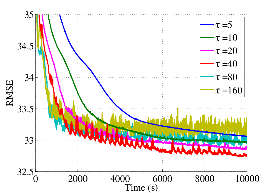
We also studied how the delay limit affects the performance of ADVGP. Practically, when many machines are used, some worker may always be slower than the others due to environmental factors, e.g., unbalanced workloads. To simulate this scenario, we intentionally introduced a latency by assigning each worker a random sleep time of , or seconds at initialization; hence a worker would pause for its given sleep time before each iteration. In our experiment, the average per-iteration running time was only seconds; so the fastest worker could be hundreds of iterations ahead of the slowest one in the asynchronous setting. We examined and plotted RMSEs as a function of time in Figure 2. Since RMSE of the synchronous case () is much larger than the others, we do not show it in the figure. When is larger, ADVGP’s performance is more fluctuating. Increasing , we first improved the prediction accuracy due to more efficient CPU usage; however, later we observed a decline caused by the excessive asynchronization that impaired the optimization. Therefore, to use ADVGP for workers at various paces, we need to carefully choose the appropriate delay limit .
6.2 Scalability
Next, we examined the scalability of our asynchronous inference method, ADVGP. To this end, we used the K/K dataset and compared with the synchronous inference algorithm DistGP (Gal et al., 2014). For a fair comparison, we used the local gradient descent version of DistGP, i.e., DistGP-GD. We conducted two experiments on 4 c4.8xlarge instances of Amazon EC2 cloud, where we set the number of inducing points . In the first experiment, we fixed the size of the training data, and increased the number of CPU cores from to . We examined the per-iteration running time of both ADVGP and DistGP-GD. Figure 3(A) shows that while both decreasing with more CPU cores, the per-iteration running time of ADVGP is much less than that of DistGP-GD. This demonstrates the advantage of ADVGP in computational efficiency. In addition, the per-iteration running time of ADVGP decays much more quickly than that of DistGP-GD as the number of cores approaches . This implies that even the communication cost becomes dominant, the asynchronous mechanism of ADVGP still effectively reduces the latency and maintains a high usage of the computational power. In the second experiment, we simultaneously increased the number of cores and the size of training data. We started from K samples and cores and gradually increased them to K samples and cores. As shown in Figure 3(B), the average per-iteration time of DistGP-GD grows linearly; in contrast, the average per-iteration time of ADVGP stays almost constant. We speculate that without synchronous coordination, ADVGP can fully utilize the network bandwidth so that the increased amount of messages, along with the growth of the data size, affect little the network communication efficiency. This demonstrates the advantage of asynchronous inference from another perspective.
 |
 |
| (A) | (B) |
6.3 NYC Taxi Traveling Time Prediction
Finally, we applied ADVGP for an extremely large problem: the prediction of the taxi traveling time in New York city. We used the New York city yellow taxi trip dataset 22 2 http://www.nyc.gov/html/tlc/html/about/trip_record_data.shtml, which consist of billions of trip records from January 2009 to December 2015. We excluded the trips that are outside the NYC area or more than 5 hours. The average traveling time is 764 seconds and the standard derivation is 576 seconds. To predict the traveling time, we used the following 9 features: time of the day, day of the week, day of the month, month, pick-up latitude, pick-up longitude, drop-off latitude, drop-off longitude, and travel distance. We used Amazon EC2 cloud, and ran ADVGP on multiple Amazon c4.8xlarge instances, each with 36 vCPUs and 60 GB memory. We compared with the linear regression model implemented in Vowpal Wabbit (Agarwal et al., 2014). Vowpal Wabbit is a state-of-the-art large scale machine learning software package and has been used in many industrial-scale applications, such as click-through-rate prediction (Chapelle et al., 2014).
We first randomly selected M training samples and K test samples. We set and initialized the inducing points as the the K-means cluster centers from a subset of M training samples. We trained a GP regression model with ADVGP, using Amazon instances with processes. The delay limit was selected as . We used Vowpal Wabbit to train a linear regression model, with default settings. We also took the average traveling time over the training data to obtain a simple mean prediction. In Figure 4(A), we report RMSEs of the linear regression and the mean prediction, as well as the GP regression along with running time. As we can see, ADVGP greatly outperforms the competing methods. Only after minutes, ADVGP has improved RMSEs of the linear regression and the mean prediction by and , respectively; the improvements continued for about minutes. Finally, ADVGP reduced the RMSEs of the linear regression and the mean prediction by and , respectively. The RMSEs are {ADVGP: , linear regression: , mean-prediction: }.
 |
 |
| (A) 100M training samples | (B) 1B training samples |
To further verify the advantage of GP regression in extremely large applications, we used B training and M testing samples. We used inducing points, initialized by the K-means cluster centers from a M training subset. We ran ADVGP using Amazon instances with processes and chose . As shown in Figure 4(B), the RMSE of GP regression outperforms the linear models by a large margin. After minutes, ADVGP has improved the RMSEs of the linear regression and the mean prediction by and , respectively; the improvement kept growing for about hours. At the convergence, ADVGP outperforms the linear regression and the mean prediction by and , respectively. The RMSEs are {ADVGP: , linear regression: , mean-prediction: }. In addition, the average per-iteration time of ADVGP is only seconds. These results confirm the power of the nonlinear regression in extremely large real-world scenarios, comparing with linear models, while the latter are much easier to be scaled up and hence more popular.
7 Conclusion
We have presented ADVGP, an asynchronous, distributed variational inference algorithm for GP regression, which enables real-world extremely large applications. ADVGP is based on a novel variational GP framework, which allows flexible construction of low rank approximations and can relate to many sparse GP models.
References
- Agarwal and Duchi (2011) Agarwal, A. and Duchi, J. C. (2011). Distributed delayed stochastic optimization. In Advances in Neural Information Processing Systems 24, pages 873–881. Curran Associates, Inc.
- Agarwal et al. (2014) Agarwal, A., Chapelle, O., Dudík, M., and Langford, J. (2014). A reliable effective terascale linear learning system. Journal of Machine Learning Research, 15, 1111–1133.
- Bauer et al. (2016) Bauer, M., van der Wilk, M., and Rasmussen, C. E. (2016). Understanding probabilistic sparse Gaussian process approximations. In Advances in Neural Information Processing Systems 29, pages 1525–1533.
- Bishop and Tipping (2000) Bishop, C. M. and Tipping, M. E. (2000). Variational relevance vector machines. In Proceedings of the 16th Conference in Uncertainty in Artificial Intelligence (UAI).
- Chapelle et al. (2014) Chapelle, O., Manavoglu, E., and Rosales, R. (2014). Simple and scalable response prediction for display advertising. ACM Transactions on Intelligent Systems and Technology (TIST), 5(4), 61:1–61:34.
- Dai et al. (2014) Dai, Z., Damianou, A., Hensman, J., and Lawrence, N. D. (2014). Gaussian process models with parallelization and GPU acceleration. In NIPS Workshop on Software Engineering for Machine Learning.
- Deisenroth and Ng (2015) Deisenroth, M. and Ng, J. W. (2015). Distributed Gaussian processes. In Proceedings of the 32nd International Conference on Machine Learning, pages 1481–1490.
- Filippone et al. (2013) Filippone, M., Zhong, M., and Girolami, M. (2013). A comparative evaluation of stochastic-based inference methods for gaussian process models. Machine Learning, 93(1), 93–114.
- Gal et al. (2014) Gal, Y., van der Wilk, M., and Rasmussen, C. (2014). Distributed variational inference in sparse Gaussian process regression and latent variable models. In Advances in Neural Information Processing Systems 27, pages 3257–3265.
- Hensman et al. (2013) Hensman, J., Fusi, N., and Lawrence, N. D. (2013). Gaussian processes for big data. In Proceedings of the Conference on Uncertainty in Artificial Intelligence (UAI).
- Hensman et al. (2015) Hensman, J., Matthews, A. G., Filippone, M., and Ghahramani, Z. (2015). Mcmc for variationally sparse gaussian processes. In Advances in Neural Information Processing Systems, pages 1648–1656.
- Kumar et al. (2009) Kumar, S., Mohri, M., and Talwalkar, A. (2009). Ensemble Nyström method. In Y. Bengio, D. Schuurmans, J. D. Lafferty, C. K. I. Williams, and A. Culotta, editors, Advances in Neural Information Processing Systems 22, pages 1060–1068. Curran Associates, Inc.
- Li et al. (2013) Li, M., Andersen, D. G., and Smola, A. J. (2013). Distributed delayed proximal gradient methods. In NIPS Workshop on Optimization for Machine Learning.
- Li et al. (2014a) Li, M., Andersen, D. G., Smola, A., and Yu, K. (2014a). Communication efficient distributed machine learning with the parameter server. In Neural Information Processing Systems 27.
- Li et al. (2014b) Li, M., Andersen, D. G., Park, J. W., Smola, A. J., Ahmed, A., Josifovski, V., Long, J., Shekita, E. J., and Su, B.-Y. (2014b). Scaling distributed machine learning with the parameter server. In 11th USENIX Symposium on Operating Systems Design and Implementation (OSDI 14), pages 583–598.
- Matthews et al. (2017) Matthews, A. G. d. G., van der Wilk, M., Nickson, T., Fujii, K., Boukouvalas, A., León-Villagrá, P., Ghahramani, Z., and Hensman, J. (2017). GPflow: A Gaussian process library using TensorFlow. Journal of Machine Learning Research, 18(40), 1–6.
- Murray and Adams (2010) Murray, I. and Adams, R. P. (2010). Slice sampling covariance hyperparameters of latent gaussian models. In Advances in Neural Information Processing Systems 24, pages 1732–1740.
- Peng and Qi (2015) Peng, H. and Qi, Y. (2015). EigenGP: Sparse Gaussian process models with adaptive eigenfunctions. In Proceedings of the 24th International Joint Conference on Artificial Intelligence, pages 3763–3769.
- Quiñonero-Candela and Rasmussen (2005) Quiñonero-Candela, J. and Rasmussen, C. E. (2005). A unifying view of sparse approximate Gaussian process regression. The Journal of Machine Learning Research, 6, 1939–1959.
- Rasmussen and Williams (2006) Rasmussen, C. E. and Williams, C. K. I. (2006). Gaussian Processes for Machine Learning. The MIT Press.
- Schwaighofer and Tresp (2003) Schwaighofer, A. and Tresp, V. (2003). Transductive and inductive methods for approximate Gaussian process regression. In Advances in Neural Information Processing Systems 15, pages 953–960. MIT Press.
- Seeger et al. (2003) Seeger, M., Williams, C., and Lawrence, N. (2003). Fast forward selection to speed up sparse Gaussian process regression. In Proceedings of the Ninth International Workshop on Artificial Intelligence and Statistics.
- Smola and Bartlett (2001) Smola, A. J. and Bartlett, P. L. (2001). Sparse greedy Gaussian process regression. In Advances in Neural Information Processing Systems 13. MIT Press.
- Snelson and Ghahramani (2005) Snelson, E. and Ghahramani, Z. (2005). Sparse Gaussian processes using pseudo-inputs. In Advances in Neural Information Processing Systems, pages 1257–1264.
- Titsias (2009) Titsias, M. K. (2009). Variational learning of inducing variables in sparse Gaussian processes. In Proceedings of the Twelfth International Conference on Artificial Intelligence and Statistics, pages 567–574.
- Williams and Seeger (2001) Williams, C. and Seeger, M. (2001). Using the Nyström method to speed up kernel machines. In Advances in Neural Information Processing Systems 13, pages 682–688.
- Zeiler (2012) Zeiler, M. D. (2012). ADADELTA: an adaptive learning rate method. arXiv:1212.5701.
Appendices
Appendix A Derivatives
A.1 Objective
As described in the paper, the objective function to be minimized is where
| (23) | ||||
| (24) |
and we define and .
A.2 Kernel
A common choice for the kernel is the anisotropic squared exponential covariance function:
| (25) |
in which the hyperparameters are the signal variance and the lengthscales , controlling how fast the covariance decays with the distance between inputs. Using this covariance function, we can prune input dimensions by shrinking the corresponding lengthscales based on the data (when , the -th dimension becomes totally irrelevant to the covariance function value). This pruning is known as Automatic Relevance Determination (ARD) and therefore this covariance is also called the ARD squared exponential.
Derivative over
The derivative of over is
| (26) |
Derivative over
The derivative of over is
| (27) |
Derivative over
By defining the lower triangular Cholesky factor of , the derivative of over is
| (28) |
where
| (29) | ||||
| (30) |
The symbol denotes the Hadamard product, and is an upper triangular matrix with diagonal elements all equal to and strictly upper triangular elements all equal to , as follows:
Derivative over
The derivative of over is
| (36) |
Appendix B Properties of the ELBO of ADVGP
By defining as the upper triangular Cholesky factor of , i.e., , we have
Lemma B.1.
The gradient of in Equation 23, , is Lipschitz continuous with respect to each element in and .
We can prove this by showing the first derivative of with respect to each element of and is bounded, which is constant in our case. As shown in our paper, the gradients of with respect to and are:
| (37) | ||||
| (38) |
which are affine functions for and respectively. Therefore, the first derivative of is constant.
Lemma B.2.
in Equation 24 is a convex function with respect to and .
This can be proved by verifying that the Hessian matrices of with respect to and are both positive semidefinite, where we denote as the operator that stacks the columns of a matrix as a vector. To show this, we first compute the partial derivatives of with respect to and as
| (39) | ||||
| (40) |
The Hessian matrix of with respect to is
| (41) |
The Hessian matrix of with respect to is
| (42) |
where , and .
Appendix C Negative Log Evidences on US Flight Data
 |
 |
| (A) | (B) |
| Method | ||
|---|---|---|
| ADVGP | ||
| DistGP-GD | ||
| DistGP-LBFGS |
 |
 |
| (A) | (B) |
| Method | ||
|---|---|---|
| ADVGP | ||
| DistGP-GD | ||
| DistGP-LBFGS |
Appendix D Mean Negative Log Predictive Likelihoods (MNLPs) on US Flight Data
 |
 |
| (A) | (B) |
| Method | ||
|---|---|---|
| ADVGP | ||
| DistGP-GD | ||
| DistGP-LBFGS | 1.3136 | |
| SVIGP | 1.3157 | 1.3096 |
 |
 |
| (A) | (B) |
| Method | ||
|---|---|---|
| ADVGP | ||
| DistGP-GD | ||
| DistGP-LBFGS | ||
| SVIGP | 1.3335 | 1.3306 |