Batch-Expansion Training:
An Efficient Optimization Framework∗
Michał Dereziński Dept. of Computer Science UC Santa Cruz mderezin@ucsc.edu Dhruv Mahajan Facebook Research Menlo Park dhruvm@fb.com S. Sathiya Keerthi Microsoft Corporation Mountain View keerthi@microsoft.com
S. V. N. Vishwanathan Markus Weimer
Dept. of Computer Science UC Santa Cruz vishy@ucsc.edu Microsoft Corporation Mountain View mweimer@microsoft.com
Abstract
We propose Batch-Expansion Training (BET), a framework for running a batch optimizer on a gradually expanding dataset. As opposed to stochastic approaches, batches do not need to be resampled i.i.d. at every iteration, thus making BET more resource efficient in a distributed setting, and when disk-access is constrained. Moreover, BET can be easily paired with most batch optimizers, does not require any parameter-tuning, and compares favorably to existing stochastic and batch methods. We show that when the batch size grows exponentially with the number of outer iterations, BET achieves optimal data-access convergence rate for strongly convex objectives. Experiments in parallel and distributed settings show that BET performs better than standard batch and stochastic approaches.
1 Introduction
State-of-the-art optimization algorithms used in machine learning broadly tend to fall into two main categories: batch methods, which visit the entire dataset once before performing an expensive parameter update, and stochastic methods, which rely on a small subset of training data, to apply quick parameter updates at a much greater frequency. Both approaches present different trade-offs. Stochastic updates often provide very good early performance, since they can update the parameters a considerable number of times before even a single batch update finishes. On the other hand, by accessing the full dataset at each step, batch algorithms can better utilize second-order information about the loss function, while taking advantage of parallel and distributed architectures. Finding approaches that provide the best of both worlds is an important area of research. In this paper, we propose a new framework which – while closer to batch in spirit – enjoys the benefits of stochastic methods. In addition, our framework addresses a practical issue observed in real-world industrial settings, which we now describe.
In industrial server farms, compute resources for large jobs become available only in a phased manner. When running a batch optimizer, which requires loading the entire dataset, one has to wait until all the machines become available before beginning the computation. Moreover, the training data, which typically consists of user logs, is distributed across multiple locations. This data needs to be normalized, often by communicating summary statistics or subsets of the data across the network. Since stochastic optimization algorithms only deal with a subset of the data at a time, one can largely avoid the bottleneck of data normalization by preparing mini-batches at a time. However, now each data point needs to be visited multiple times randomly, and this requires performing many random accesses from a hard-disk or network attached storage (NAS), which is inherently slow. Moreover, extending stochastic optimization to the distributed setting is still an active area of research. This raises the question of whether the compute and data-availability delays could be avoided in batch methods, and how that would affect the training time.
We propose Batch-Expansion Training (BET), an adaptive, parameter-free meta-algorithm, which can be paired with most batch optimization methods to accelerate their performance in sequential, parallel, as well as distributed settings, addressing the issues discussed above. Our approach hinges on the following observation: initially, when only a subset of the data is available, the statistical error (the error that arises because one is observing a sample from the true underlying data distribution) is large. Therefore, we can tolerate a large optimization error (the error that arises because of the iterative nature of the batch optimizer). However, as the sample size increases, the statistical error decreases and the corresponding optimization error that we can tolerate also decreases. BET exploits this by initially training models with large optimization error on smaller subsets of the data, and iteratively loading more training data, and driving down the optimization error.
Relying on classical results in statistical learning theory, we show that any optimizer exhibiting linear convergence rate can be effectively accelerated by periodically doubling the data size after a certain number of iterations. We propose a simple parameter-free algorithm, which dynamically decides the optimal number of iterations between each data expansion, adapting to the performance of a batch optimizer provided as a black box method. Experiments using Nonlinear Conjugate Gradient (CG), as well as the L-BFGS method, demonstrate the versatility of our framework. We show that for strongly convex losses BET achieves the same asymptotic convergence rate as SGD in terms of data accesses (and is strictly faster than regular batch updates). However, unlike stochastic methods, BET reuses all of the data that has already been loaded, which helps it scale very well in parallel and distributed settings, as confirmed by the experimental results.
2 Related Work
There has been a recent explosion of interest in both batch and stochastic optimization methods for machine learning. Algorithms like Stochastic Variance Reduced Gradient method [15] and related approaches [22, 10] mix SGD-like steps with some batch computations to control the stochastic noise. Others have proposed to parallelize stochastic training through large mini-batches [16, 11]. However, these methods do not address the issues of compute and data-availability delays that we discussed above. Additionally, two-stage approaches have been proposed [1, 24], which employ SGD at the beginning followed by a batch optimizer (e.g., L-BFGS). These methods are much more limited than BET, which allows for multiple stages of optimization, with clear practical benefits. Interleaving computation with data loading was shown to have significant practical benefits by [18]. However, that work is confined to training on a single machine and did not provide any theoretical convergence guarantees. In contrast, we largely focus on the distributed setting and provide convergence guarantees.
Several works explore the idea of batch expansion in various forms. [7, 14] propose using stochastic mini-batches of gradually increasing size paired with optimizers like gradient descent or Newton-CG. The algorithms proposed there strongly rely on stochastic sampling, which makes them less resource-efficient than BET, and not applicable to certain distributed settings. The convergence guarantees offered in [7] are limited to using gradient descent as the inner optimizer, and heavily rely on the independence conditions present in stochastic sampling. The idea of gradually increasing batch size without resampling the batches was first discussed by [27], however their convergence analysis is also limited to gradient descent. Recently, [19, 9] proposed variants of the Newton’s method and of the SAGA [10] algorithm which run on increasing batch sizes. Both of those methods pose challenges in large-scale distributed settings (expensive hessian computation required for Newton’s method and sequential stochastic updates in SAGA). The key advantage of our meta-algorithm is that it can be used with any inner batch optimizer as a black box, including quasi-Newton methods like L-BFGS, making this approach more broadly applicable and scalable. Similarly, our complexity analysis applies to a wide range of inner optimizers.
3 Batch-Expansion Training
We consider a standard composite convex optimization problem arising in regularized linear prediction. Given a dataset , we aim to approximately minimize the average regularized loss
| (1) |
where and is the loss of predicting with a linear model against a target label . Any iterative optimization algorithm in this setting will produce a sequence of models with the goal that has small optimization error with respect to the exact optimum , where
Note that our true goal is to predict well on an unseen example coming from an underlying distribution. The right regularization for this task can be determined experimentally or from the statistical guarantees of loss function , as discussed in [25, 23]. In this paper, however, we will assume that an acceptable was chosen and concentrate on the problem of minimizing .
3.1 Linear convergence of the batch optimizer
Adding -norm regularization in function makes it -strongly convex. In this setting, many popular batch optimization algorithms enjoy linear convergence rate [21]. Namely, given arbitrary model and any , after at most iterations - where a single iteration can look at the entire dataset - we can reduce its optimization error by a multiplicative factor of , obtaining such that
Note that the runtime of a single iteration will depend on data size , but the number of needed iterations does not. Setting , we observe that only a constant number of batch iterations is necessary for a linearly converging optimizer to halve the optimization error of . This constant depends on the convergence rate enjoyed by the method. For example, in the case of batch gradient descent we need iterations to reduce the optimization error by a factor of 2 [6] (note the dependence on the strong convexity coefficient), while other methods (like L-BFGS) can achieve better rates of convergence [17]. Furthermore, the time complexity of performing a single iteration for many of those algorithms (including GD and L-BFGS) is linearly proportional to the data size. We refer to methods exhibiting both linear convergence (with respect to a given loss) and linear time complexity of a single iteration as linear optimizers. From now on, we only consider this class of methods.
3.2 Dataset size selection
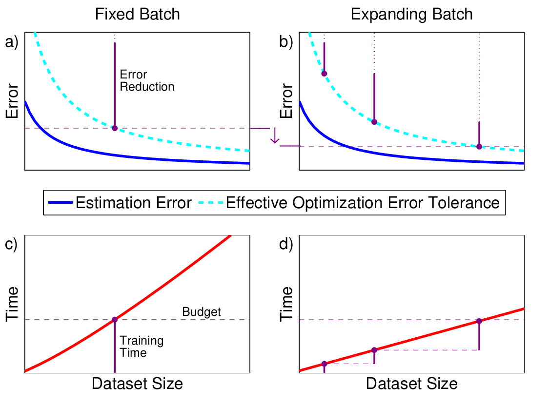
The general task of an optimization algorithm is to return a model with small optimization error . For selecting an effective optimization error tolerance in a machine learning problem, we often look at the estimation error exhibited by the objective, i.e. how much deviates from the expected regularized loss measured on a random unseen example. As discussed in [23, 5], the effective optimization error tolerance should be proportional to the estimation error of , because optimizing beyond that point does not yield any improvement on unseen data. Note that under standard statistical assumptions, the more data we use, the smaller the estimation error becomes [25], and thus, the effective optimization error tolerance should also be decreased (see Figure 1a).
Consider the scenario where data is abundant, but we have a limited time budget for training the model11 1 This is a reasonable practice in many web applications.. In this case, a practitioner would select the data size so that we can reach the smallest effective optimization error tolerance (dashed curve in Figure 1a) within the allotted training time. Vertical line in Figure 1a shows the reduction in optimization error that the algorithm has to achieve to obtain the desired tolerance. If we use a batch optimizer for this task, the training time is determined by two factors. First, as the dataset grows, each iteration takes longer (e.g. for linear optimizers the iteration time is proportional to the data size, as discussed in Section 3.1). Second, the algorithm has to perform larger number of iterations, the smaller the effective optimization error tolerance. Combined, those two effects result in training time, which, for linear optimizers, grows faster than linearly with the data size (see Figure 1c).
In this paper, we propose that instead of finding the optimal dataset size at the beginning, we first load a small subset of data, train the model until we reach the corresponding effective optimization error tolerance, then we load more data, and optimize further, etc. Vertical lines in Figure 1b illustrate how optimization error is reduced in multiple stages working with increasing data sizes. This procedure benefits from faster iterations in the early stages, as shown in Figure 1d, with vertical lines corresponding to the training time for each data size, and the horizontal line showing the time budget (note that the budget shown for this method is the same as the one used in Figure 1c). Thus, our approach is able to reach smaller effective optimization error tolerance within the same time budget compared to fixing the dataset size at the beginning (see Figures 1a and 1b).
3.3 Exponentially increasing batches
We now precisely formulate the idea of training with gradually increasing data size. Suppose our goal is to return a model with optimization error . In the procedure described above, we seek to obtain a sequence of gradually improving models before we reach . Any of the intermediate models (say, model for ) has a large optimization error relative to , so to compute we can minimize an objective function with correspondingly large estimation error. Thus, we will first obtain with optimization error22 2 The optimization error for intermediate models is computed using only the loaded portion of the data. using data points, next we pick a smaller error tolerance and bigger data size , computing a better model , etc. so that in the end we reach . Algorithm 1 demonstrates a simple instantiation of this strategy, where at each stage we double the data size:
The basis for the number of inner iterations will be explained below. Note that at stage of the process we are working with an estimate of the loss function
which tends to with increasing . At this stage, the optimizer is in fact converging to an approximate optimum
rather than to the minimizer of , . To decide how much data is needed at each stage we will describe the relationship between data size and the desired optimization error . Note that model obtained at stage is assumed to satisfy , where represents optimization error for the given data subset, i.e. When going to the next stage, the data size increases, and thus we can use optimization error function , which is a better estimate of than is. In Appendix A.1, we show that function can be uniformly bounded by , plus an additional term which can be interpreted as the estimation error (of with respect to ):
| (2) |
As discussed earlier, the effective optimization error for data size is proportional to the estimation error suffered by , hence it is sufficient to demand that
| (3) |
Note that this makes the optimization error tolerance inversely proportional to the subset size , confirming our intuition that for , since , we can work with a batch of size that is smaller than .
To establish the correct rate of growth for the data size , we combine (3) with the observations made in Section 3.1. First, note that the rate of decay of sequence should match the convergence rate of the optimization algorithm, so that inequality can be satisfied for all . Recall from Section 3.1, that a linear optimizer takes only a constant number of iterations to reduce the optimization error by a constant factor. Suppose that improvement by a factor of takes iterations (going from to ). Then, using (2) and (3) we have
This suggests the following simple strategy: at each stage perform iterations of the optimizer, then divide the tolerance level by 2 (matching the convergence rate). Note that based on Equation (3), this corresponds to doubling the data size . Thus, we obtain the following simple scheme for data expansion, which maintains the desired relationship between and :
It is important that grows exponentially with . This allows for a considerable improvement in runtime. Let us say that and stages are needed to reach the final desired tolerance , i.e. . Moreover, using (3) the suitable size of the full dataset is . If we assume that one iteration of the linear optimizer takes time proportional to the data size, then the time complexity of the optimization when using batch-expansion is given by
On the other hand, when running the same optimizer on full dataset from the beginning, the time complexity becomes
Note that to establish convergence of the proposed algorithm, it is only required that the dataset is randomly permuted, i.e. that each subset represents a random portion of the data. However, the batches used in different stages do not need to be independent of each other, which is why we can reuse data from previous stages. Section 4 precisely formulates the ideas discussed above, and a careful analysis of the time complexity is given in Theorem 4.1.
3.4 Two-track algorithm
How many iterations of the proposed expansion procedure should be performed at each stage? From our high-level analysis, we concluded that a roughly constant number of updates should be sufficient for any stage (using a linear optimizer), since each time we aim to make the same multiplicative improvement to the optimization error suffered by our model. However, that constant may depend on the type of loss function, the dataset, as well as the optimizer used, and moreover, in practice the right number of iterations may in fact vary to some extent between the stages. Therefore, we need a practical method of deciding the right time to double the data. Consider the following experiment: we run two optimization tracks in parallel, first one for the batch of size , the other for half of that batch. One update on the bigger batch takes longer than an update on the smaller one. Which track will make better progress towards the optimum of the bigger batch in the same amount of time? If the starting model is far enough from the optimum , then the faster updates will initially have an advantage. However, as the convergence proceeds, only the slower track can get arbitrarily close, so at some point it will move ahead of the fast one (in terms of the loss ). Denote the starting model as . The secondary track (running on half of the batch) also starts at the same point, denoted as , and they are both updated:
where is one step of the optimizer, with respect to model , on the batch . Let and be the total runtimes of the first and second track after iterations, respectively, and let be the number of iterations that the slower track completes in the time it took the faster track to do . To compare the performance of the two tracks we will use the condition:
| (4) |
Algorithm 2 describes Batch-Expansion Training implemented using the Two-Track strategy. Note that in this algorithm we run the two tracks sequentially, in an alternating order, however running them in parallel would further improve the overall performance.
3.5 Discussion
We found that the choice to increase data size by a factor of at each stage (rather than by a different factor) is not crucial for the optimization performance (both theoretically and in practice), therefore this parameter does not require tuning. The initial subset size also does not affect performance significantly - generally, the larger we select, the more updates will be performed before first data expansion, but as long as the initial subset is small enough, total optimization time will remain close to optimal. Thus, Algorithm 2 does not require any tuning to achieve good performance. Moreover, our method can be paired with many popular batch optimizers, and it will automatically adapt its behavior to the selected inner optimizer, as shown in Section 5.1.
It is important to note that the fraction of data accessed by the algorithm is only gradually expanded as optimization proceeds. Moreover, BET iterates multiple times over the data points that have already been loaded. Thus, it is very resource efficient in a way that can be beneficial with:
Slow disk-access. Loading data from disk to memory can be a significant bottleneck [18]. Performing multiple iterations over the data points while extra data is being loaded in parallel provides speed-up.
Resource ramp-up. In distributed computing, often not all resources are made available immediately at the beginning of the optimization [20], which similarly leads to gradual data availability.
4 Complexity Analysis
In this section, we provide theoretical guarantees for the time complexity of Batch-Expansion Training and compare them to other approaches. For the remainder of this section, we assume that the inner optimizer for some and for every exhibits linear convergence:
For the sake of complexity analysis, we discuss a parameterized variant of our approach, described in Algorithm 3, and establish complexity results for it. Here, the number of updates needed at each stage is a fixed parameter .
Assumptions. We assume that the feature mapping (see (1) and the discussion below it) is -bounded, i.e. it satisfies , and that the loss function is -Lipschitz in for all . Moreover, we will use the fact that is -strongly convex, due to the use of -norm regularization. The result below holds with high probability with respect to a random permutation of data.
Theorem 4.1
Proof Recall that we denote the approximation error estimate at stage by and the full approximation error as . Moreover, note that Algorithm 3 defines the optimization error tolerances recursively as . First, we give the following uniform convergence result:
Lemma 1
For any , there exists such that
and with probability , for all and all :
| (5) | ||||
| (6) | ||||
| (7) |
See Appendix A.1 for proof. Next, using this lemma, we show the main result. Let be the convergence rate of the inner optimizer. Recall, that we set the number of inner iterations of Algorithm 3 to be
This gives us the following bound for the progress that the inner optimizer makes at each stage (for any ):
Suppose that satisfies Lemma 1. We can show by induction that (with probability ) for all , model is an -approximate solution for , i.e. that . Base case is given by (5). The inductive step follows from:
Next, we verify that is an -approximate solution for :
Finally, we move on to complexity analysis. The number of iterations in the algorithm is , since:
Assuming that one update of the inner optimizer requires passes over the data, we obtain the data-access complexity:
See Appendix A.2 for details regarding the log terms.
Using gradient descent as the inner optimizer, we have , so Algorithm 3 reaches data-access complexity . However, the general nature of this approach allows us to choose a different linear optimizer with better guarantees, like for accelerated gradient descent. Methods like L-BFGS and other approximate Newton algorithms have been shown to exhibit linear convergence [17, 12] with a rate that does not suffer from such strict dependence on the strong convexity coefficient . Hence, when using those optimizers, for most problems we should expect to be a small constant factor, in which case data-access complexity becomes .
5 Experiments

In this section we present experimental results showing the benefits of applying BET acceleration to batch optimizers and demonstrating scalability of the method in parallel and distributed settings. As the optimization problem we use logistic loss with -norm regularization trained on several standard LIBSVM datasets (see Table 1). All algorithms start with the initial model vector set to all zeros. BET was implemented as shown in Algorithm 2, without any parameters that required tuning. The results are presented using test set accuracy and training objective, the latter being shown in terms of the log Relative Functional Value Difference
| (8) |
All algorithms were implemented in the PETSc [2, 3, 4] framework, with the data split between multiple computing cores to achieve parallelization speed-up (we used 16 cores in most experiments). For splice-site dataset33 3 Due to resource constraints, we used a 1.5TB portion of the full 3TB splice-site dataset., data was additionally divided between multiple machines.
| Dataset, size | Train/Test | Dim. | |
|---|---|---|---|
| url, 1GB | 1.8M/0.5M | 3.2M | 1e-8 |
| covtype, 19GB | 0.5M/69k | 170k | 1e-6 |
| webspam, 30GB | 250k/100k | 16.6M | 1e-6 |
| splice-site, 1.5TB | 25M/4.6M | 11.7M | 2e-10 |
5.1 Adapting to inner optimizers
To demonstrate the flexibility of our framework, in this section we use two different inner optimizers with BET:
- 1.
Nonlinear Conjugate Gradient method (CG), using Fletcher-Reeves [13] formula, with exact line-search;
- 2.
Limited-memory BFGS (L-BFGS) [8].
Both of those methods are linear optimizers that employ strategies for enhancing the basic gradient descent direction. Note, that CG uses a memory vector updated at each iteration. When the loss function changes from to , one might expect that memory vector to become invalid, rendering CG ineffective. However, BET still proves very effective at accelerating memory-based algorithms.
Figure 2 shows the performance comparison of using BET with the two inner optimizers on webspam dataset, contrasted with both of them ran in regular batch mode. First, we can see that L-BFGS is a much more effective optimizer than Nonlinear CG, thus in all of the following experiments we used L-BFGS as the inner optimizer. However, both methods significantly benefit from BET. In fact, in the early phase of the optimization, performance of BET is similar with either of the optimizers. However, once batch expansion reaches close to the full dataset, quality of the underlying optimizer starts to play an important role. Circular dots on the BET plots in Figure 2 mark the points when batch size is doubled during the optimization. We observed that the average number of iterations per stage of BET is larger when the inner optimizer is CG. This matches our expectation, since theory suggests that the number of iterations per stage should be inversely proportional to the convergence rate of the inner optimizer. Moreover, within one optimization run, we saw significant fluctuations in the number of iterations needed before each batch-expansion stage, which means that there is no universal number of iterations per stage which will work well in all settings. Thus, the adaptive capabilities of the two-track algorithm are crucial to achieving good performance of batch-expansion.
5.2 Combining the benefits of batch and stochastic

In this experiment, we examine the trade-offs between batch and stochastic methods, showing how BET fits into this comparison. A batch optimizer typically starts off slower than a stochastic one, but once it gets closer to the optimum, we expect to see a fast convergence behavior. Thus, depending on which tolerance level we select, we would choose the appropriate optimizer. This is shown on a sample plot for the covtype dataset in Figure 3, where we use Parallel SGD [28] as the stochastic algorithm and L-BFGS as the Batch method, with all algorithms running on a 16 core machine (for the sake of clarity, only a portion of the full convergence time is shown). We also tested mini-batch SVRG as an alternative stochastic approach. However, due to the high communication cost, this method exhibited much slower per iteration time, and for this reason we did not include the results in the paper. To obtain the reported performance for Parallel SGD we had to tune the step size on a chunk of data, which adds to the overall optimization time, whereas BET is a parameter-free method. Our algorithm gets the best of both worlds, since it behaves like a stochastic method at the beginning, and then like a batch method towards the end. More plots are presented in Appendix B, showing datasets which favor either batch or stochastic methods. In summary, BET performs as well as the best method for each dataset, with no tuning necessary.
5.3 Parallelization speed-up

The goal of this experiment is to analyze the parallelization speed-up of BET and compare it with the speed-up of Batch. We set this up as follows: we run to convergence and find the final accuracy, then for each method, we vary the number of cores and measure the time it takes to reach within 0.25% of optimum accuracy. For this experiment we selected the url dataset to demonstrate a stark contrast with Parallel SGD. The method achieves close to linear speed-up only for up to 4 cores, after which its performance flattens. This behavior can be atributed to the fact that as we increase the number of cores, a single iteration of Parallel SGD becomes less and less effective, which in some cases may negate the parallelization speed-up altogether. Batch methods, on the other hand, behave much more reliably with parallelization, because their iterations produce the same effect regardless of the number of cores. Figure 4 shows the speed-up factors for BET, Batch and Parallel SGD. BET achieves similar speed-up as Batch, due to the fact that parallelization happens in the inner optimizer, which is the same for both methods.
5.4 Distributed optimization
Batch optimization shows the most benefits when dealing with large-scale datasets, which do not fit into the memory of a single machine. BET easily scales up to this setting as seen in Figure 5, running on the splice-site data, with 20 machines, and 50 cores per machine, compared against Batch and Parallel SGD in the same setup. Since the dataset is highly skewed, the results are shown in terms of area under Precision-Recall curve (auPRC).

Note that BET reaches close to optimum test auPRC much more quickly than Batch or Parallel SGD. Moreover, until that point batch-expansion has not reached the full training data, which means that if the data were loaded in parallel with the optimization, the optimization time would be partially absorbed into the loading time. In our experiments, each one of the 1000 processes independently reads a separate chunk of data, however this procedure still takes at least 1500 seconds even on a high-performance cluster. Thus, a portion of BET’s optimization time can be absorbed into data loading.
6 Conclusions
We proposed Batch-Expansion Training, a simple parameter-free method of accelerating batch optimizers in a way that is both theoretically and experimentally efficient. BET does not require tuning and can be paired with any optimizer, offering advantages in parallel and distributed settings. Extending our framework to non-convex optimization is an interesting direction for future research.
References
- [1] Alekh Agarwal, Olivier Chapelle, Miroslav Dudík, and John Langford. A reliable effective terascale linear learning system. J. Mach. Learn. Res., 15(1):1111–1133, January 2014.
- [2] Satish Balay, Shrirang Abhyankar, Mark F. Adams, Jed Brown, Peter Brune, Kris Buschelman, Lisandro Dalcin, Victor Eijkhout, William D. Gropp, Dinesh Kaushik, Matthew G. Knepley, Lois Curfman McInnes, Karl Rupp, Barry F. Smith, Stefano Zampini, Hong Zhang, and Hong Zhang. PETSc Web page. http://www.mcs.anl.gov/petsc, 2016.
- [3] Satish Balay, Shrirang Abhyankar, Mark F. Adams, Jed Brown, Peter Brune, Kris Buschelman, Lisandro Dalcin, Victor Eijkhout, William D. Gropp, Dinesh Kaushik, Matthew G. Knepley, Lois Curfman McInnes, Karl Rupp, Barry F. Smith, Stefano Zampini, Hong Zhang, and Hong Zhang. PETSc users manual. Technical Report ANL-95/11 - Revision 3.7, Argonne National Laboratory, 2016.
- [4] Satish Balay, William D. Gropp, Lois Curfman McInnes, and Barry F. Smith. Efficient management of parallelism in object oriented numerical software libraries. In E. Arge, A. M. Bruaset, and H. P. Langtangen, editors, Modern Software Tools in Scientific Computing, pages 163–202. Birkhäuser Press, 1997.
- [5] Leon Bottou and Olivier Bousquet. The tradeoffs of large scale learning. In Proceedings of the 20th International Conference on Neural Information Processing Systems, NIPS’07, pages 161–168, USA, 2007. Curran Associates Inc.
- [6] Sébastien Bubeck. Convex optimization: Algorithms and complexity. Found. Trends Mach. Learn., 8(3-4):231–357, November 2015.
- [7] Richard H. Byrd, Gillian M. Chin, Jorge Nocedal, and Yuchen Wu. Sample size selection in optimization methods for machine learning. Math. Program., 134(1):127–155, August 2012.
- [8] Richard H. Byrd, Peihuang Lu, Jorge Nocedal, and Ciyou Zhu. A limited memory algorithm for bound constrained optimization. SIAM Journal on Scientific Computing, 16(5):1190–1208, 1995.
- [9] Hadi Daneshmand, Aurelien Lucchi, and Thomas Hofmann. Starting small - learning with adaptive sample sizes. In Maria Florina Balcan and Kilian Q. Weinberger, editors, Proceedings of The 33rd International Conference on Machine Learning, volume 48 of Proceedings of Machine Learning Research, pages 1463–1471, New York, New York, USA, 20–22 Jun 2016. PMLR.
- [10] Aaron Defazio, Francis R. Bach, and Simon Lacoste-Julien. SAGA: A fast incremental gradient method with support for non-strongly convex composite objectives. In Advances in Neural Information Processing Systems 27: Annual Conference on Neural Information Processing Systems 2014, December 8-13 2014, Montreal, Quebec, Canada, pages 1646–1654, 2014.
- [11] Ofer Dekel, Ran Gilad-Bachrach, Ohad Shamir, and Lin Xiao. Optimal distributed online prediction using mini-batches. J. Mach. Learn. Res., 13(1):165–202, January 2012.
- [12] Murat A. Erdogdu and Andrea Montanari. Convergence rates of sub-sampled newton methods. In Proceedings of the 28th International Conference on Neural Information Processing Systems, NIPS’15, pages 3052–3060, Cambridge, MA, USA, 2015. MIT Press.
- [13] R. Fletcher and C. M. Reeves. Function minimization by conjugate gradients. The Computer Journal, 7(2):149–154, February 1964.
- [14] Michael P. Friedlander and Mark Schmidt. Hybrid deterministic-stochastic methods for data fitting. SIAM Journal on Scientific Computing 34(3), 2012.
- [15] Rie Johnson and Tong Zhang. Accelerating stochastic gradient descent using predictive variance reduction. In Christopher J. C. Burges, Léon Bottou, Zoubin Ghahramani, and Kilian Q. Weinberger, editors, NIPS, pages 315–323, 2013.
- [16] Mu Li, Tong Zhang, Yuqiang Chen, and Alexander J. Smola. Efficient mini-batch training for stochastic optimization. In Proceedings of the 20th ACM SIGKDD International Conference on Knowledge Discovery and Data Mining, KDD ’14, pages 661–670, New York, NY, USA, 2014. ACM.
- [17] Chih-Jen Lin, Ruby C. Weng, and S. Sathiya Keerthi. Trust region newton methods for large-scale logistic regression. In Proceedings of the 24th International Conference on Machine Learning, ICML ’07, pages 561–568, New York, NY, USA, 2007. ACM.
- [18] Shin Matsushima, S.V.N. Vishwanathan, and Alexander J. Smola. Linear support vector machines via dual cached loops. In Proceedings of the 18th ACM SIGKDD International Conference on Knowledge Discovery and Data Mining, KDD ’12, pages 177–185, New York, NY, USA, 2012. ACM.
- [19] Aryan Mokhtari, Hadi Daneshmand, Aurélien Lucchi, Thomas Hofmann, and Alejandro Ribeiro. Adaptive newton method for empirical risk minimization to statistical accuracy. In Advances in Neural Information Processing Systems 29: Annual Conference on Neural Information Processing Systems 2016, December 5-10, 2016, Barcelona, Spain, pages 4062–4070, 2016.
- [20] Shravan Narayanamurthy, Markus Weimer, Dhruv Mahajan, Tyson Condie, Sundararajan Sellamanickam, and Keerthi Selvaraj. Towards resource-elastic machine learning. NIPS 2013 BigLearn Workshop, 2013.
- [21] Jorge Nocedal and Steve J. Wright. Numerical optimization. Springer Series in Operations Research and Financial Engineering. Springer, Berlin, 2006. NEOS guide http://www-fp.mcs.anl.gov/otc/Guide/.
- [22] Mark Schmidt, Nicolas Le Roux, and Francis Bach. Minimizing finite sums with the stochastic average gradient. Math. Program., 162(1-2):83–112, March 2017.
- [23] Shai Shalev-Shwartz and Nathan Srebro. Svm optimization: Inverse dependence on training set size. In Proceedings of the 25th International Conference on Machine Learning, ICML ’08, pages 928–935, New York, NY, USA, 2008. ACM.
- [24] Shai Shalev-Shwartz and Tong Zhang. Stochastic dual coordinate ascent methods for regularized loss. J. Mach. Learn. Res., 14(1):567–599, February 2013.
- [25] Karthik Sridharan, Shai Shalev-shwartz, and Nathan Srebro. Fast rates for regularized objectives. In D. Koller, D. Schuurmans, Y. Bengio, and L. Bottou, editors, Advances in Neural Information Processing Systems 21, pages 1545–1552. Curran Associates, Inc., 2009.
- [26] Ilya Tolstikhin, Nikita Zhivotovskiy, and Gilles Blanchard. Permutational rademacher complexity. In Proceedings of the 26th International Conference on Algorithmic Learning Theory - Volume 9355, pages 209–223, New York, NY, USA, 2015. Springer-Verlag New York, Inc.
- [27] Martin Zinkevich. Theoretical analysis of a warm start technique. NIPS 2011 BigLearn Workshop, 2011.
- [28] Martin Zinkevich, Markus Weimer, Alexander J. Smola, and Lihong Li. Parallelized Stochastic Gradient Descent. In John D. Lafferty, Christopher K. I. Williams, John S. Taylor, Richard S. Zemel, and Aron Culotta, editors, NIPS, pages 2595–2603. Curran Associates, Inc., 2010.
Appendix A Proof Details for Theorem 4.1
A.1 Proof of Lemma 1
First, we formulate a uniform-convergence bound, which closely resembles Theorem 1 from [25]. The only difference is that they consider PAC setting: sampling an i.i.d. dataset from a fixed distribution, and comparing the finite-sample objective computed using with the true objective , which is an expectation over the distribution. On the other hand, we consider an increasing sequence of datasets , selected by a uniformly random permutation of the full dataset . Note, that we assume the algorithm never observes the full dataset, only loading as much data as needed. Taking the limit of , the relationship between any subset and the full dataset becomes statistically equivalent to i.i.d. sampling from any fixed underlying distribution. Given that our goal is generalization to predicting on new data, that simplification is reasonable, although the analysis does go through in the strict optimization setting, where is finite. However, even with this assumption, we still need to describe the relationship between two consecutive subsets in the sequence, which does not fit the i.i.d. sampling model. To that end, we can view as a fraction of elements from , selected uniformly at random without replacement. We now describe the relationship between the two consecutive loss estimates in this sequence. Note, that in this section the big- notation hides only fixed numeric constants.
Lemma 2
With probability , for all and all we have
| (9) |
Proof The proof is very similar to [25], except we replace standard Rademacher Complexity with Permutational Rademacher Complexity (PRC), proposed in [26]. Let us fix , and consider a specific set of instances , from which a random subset is sampled (without replacement). Following [25], for any we define
where
and
Our aim is to analyze the empirical average of the function values from evaluated on a given instance set :
We can translate the task of comparing and to describe it in terms of the function class :
To compare with we use Theorem 5 [26], which provides transductive risk bounds through expected PRC of function class , conditioned on set :
Here, the randomness only comes from selecting as a subset of . For any , with probability at least ,
Note, that (see [26]), where is the standard Rademacher Complexity. The remainder of the proof proceeds identically as in [25] (up to numerical constants), i.e. by bounding both terms and by
Note, that since the bound is obtained for every possible , it will still hold with probability at least without conditioning on .
Finally, as shown in [25], by setting appropriately we obtain that w.p. , for all
Applying union bound to account for all values of simultaneously, we obtain the desired result.


We return to the proof of Lemma 1. Using Lipschitz and boundedness assumptions for the loss and mapping , as well as strong convexity of the regularized objective, we obtain initial tolerance of the loss estimate:
We used the fact that is set to zero only for applying inequality to drop the regularization terms (any initialization satisfying that requirement is acceptable).
Finally, Condition (7) regards the relationship between approximation error estimate and full approximation error . This bound can be obtained by repeating the same argument as in Lemma 2. We can either assume and use standard Rademacher complexity, as in Theorem 1, [25], or stay with the finite optimization model and apply PRC. Thus, we can set to satisfy the conditions of Lemma 1.
A.2 Deriving Log Terms in Theorem 4.1
The number of iterations, , depends on . But in Lemma 1 we defined using . To address this, we have to find satisfying:
with . It is easy to show that for small enough it suffices to set
Thus, setting , we obtain the final complexity bound in Theorem 4.1 as
Appendix B Additional Experiments
| Dataset, size | Train/Test | Dim. | |
|---|---|---|---|
| HIGGS, 8GB | 10.5M/0.5M | 28 | 1e-10 |
| url, 1GB | 1.8M/0.5M | 3.2M | 1e-8 |
In this section we look at two datasets with very different properties. First one, HIGGS, is large, but extremely low dimensional. In this case, given an overabundance of data, if we look at the accuracy plot (see Figure 6), the Batch algorithm takes much longer to converge than Parallel SGD. This follows from the fact that the task has low sample complexity, and a Batch method is wasting resources by training on too much data. The second dataset, url, is very high-dimensional, and in this case Batch has clear advantage over SGD. BET does as well as the best method on each dataset. In the case of HIGGS, BET simply converges to the optimum accuracy before it even reaches full dataset, thus saving on expensive iterations. For url, the batch expansion happens relatively early on in the optimization, and from that point on the algorithm is simply running full L-BFGS. Those two extreme cases show the versatility and robustness of our proposed meta-algorithm.