The Discrete Empirical Interpolation Method: Canonical Structure and Formulation in Weighted Inner Product SpacesThanks: The work of the first author was supported by grant HRZZ-9345 from the Croatian Science Foundation.
Abstract
New contributions are offered to the theory and numerical implementation of the Discrete Empirical Interpolation Method (DEIM). A substantial tightening of the error bound for the DEIM oblique projection is achieved by index selection via a strong rank revealing QR factorization. This removes the exponential factor in the dimension of the search space from the DEIM projection error, and allows sharper a priori error bounds. Well-known canonical structure of pairs of projections is used to reveal canonical structure of DEIM. Further, the DEIM approximation is formulated in weighted inner product defined by a real symmetric positive-definite matrix . The weighted DEIM (-DEIM) can be interpreted as a numerical implementation of the Generalized Empirical Interpolation Method (GEIM) and the more general Parametrized-Background Data-Weak (PBDW) approach. Also, it can be naturally deployed in the framework when the POD Galerkin projection is formulated in a discretization of a suitable energy (weighted) inner product such that the projection preserves important physical properties such as e.g. stability. While the theoretical foundations of weighted POD and the GEIM are available in the more general setting of function spaces, this paper focuses to the gap between sound functional analysis and the core numerical linear algebra. The new proposed algorithms allow different forms of -DEIM for point-wise and generalized interpolation. For the generalized interpolation, our bounds show that the condition number of does not affect the accuracy, and for point-wise interpolation the condition number of the weight matrix enters the bound essentially as , where is the spectral condition number.
keywords
empirical interpolation, Galerkin projection, generalized empirical interpolation, nonlinear model reduction, oblique projection, proper orthogonal decomposition, parametrized-background data-weak approach, rank revealing QR factorization, weighted inner productAMS
15A12, 15A23, 65F35, 65L02, 65M20, 65M22, 93A15, 93B40, 93C15, 93C201 Introduction
Suppose we want to run numerical simulations of a physical reality described by a set of ordinary differential equations (ODEs)
| (1) |
where , . Often, of interest is , with some given matrix . Such a system of ODEs can arise from discretization of a spatial differential operator in time dependent PDEs (e.g. method of lines), e.g. for the purposes of prediction and/or control, or optimization with respect to a set of parameters. In a parameter dependent case we have , , , and is also parameter dependent, where the parameter , that may carry e.g. information on material properties, is from a parameter domain , .11 1 To keep the notation simple, we suppress the explicit parameter dependence until numerical experiments in §5. The function is in general assumed to be nonlinear. Large dimension (say, ) makes the task computationally intractable for multiple query problems, and one is forced to devise and use a reduced order system that emulates (1).
In a projection based model order reduction, one constructs a suitable low dimensional subspace as the range of an orthonormal matrix () and seeks an approximation of the form , . The solution is stored at a set of discrete times (also known as snapshots) and is the average over the snapshots. The matrix can be, e.g., the POD basis of the leading left singular vectors of the centered snapshots , computed at the discrete times from high resolution numerical simulations in the off-line phase; possibly over a parameter grid. It is assumed that . By enforcing the orthogonality of the residual and the space , one obtains Galerkin projection of the original problem
| (2) |
where is , , but the projected nonlinear forcing term still involves the dimension , in computing and (at a sequence of discrete values ), as well as in computing . For large , this carries substantial computational effort and heavy memory traffic.
The Discrete Empirical Interpolation (DEIM) [15] method provides a way to alleviate these burdens, and to efficiently approximate from a learned subspace. DEIM originates in the Empirical Interpolation Method (EIM) [24], [5], [42] and it uses the reduced basis provided by the POD. For a related discrete version of EIM see [26]. Here, for the reader’s convenience, we first briefly review the main steps of DEIM approximation and its error estimate, and then we place it in the more general concepts of GEIM and PBDW.
1.1 DEIM
Suppose we have empirically determined an -dimensional subspace as the range of an orthonormal such that . This can be done e.g. by the POD, which will determine a suitable dimension from the decay of the singular values of the matrix of snapshots. The tacit assumption is that is from a set of functions with small Kolmogorov -width [35], [36, Chapter 6], [42]. Inserting the orthogonal projection into (2) gives
| (3) |
where denotes the identity, and the last term (the POD error, as seen from ) can be neglected. However, this still does not solve the problem of computational complexity because it requires all components of , and the matrix vector product takes operations for every time point .
The DEIM [15] trick is to select a submatrix of the identity ,
and to replace the orthogonal projector by the oblique projector
Note that has an interpolating property at the selected coordinates, . The alternative for (3) is thus
| (4) |
where in the matrix product , the factor can be pre-computed in the off-line phase. Obviously, important is only the component of the error that lies in .
The on-line computation at any particular involves only values , . If is defined at a vector component-wise as22 2 For a general nonlinear , where () denotes a sub-array of needed to evaluate , the situation is more complicated, see [15, §3.5]. then
and the computational complexity of
becomes independent of the dimension , once the time independent matrices are precomputed in the off-line phase.33 3 In the sequel, for the sake of simplicity, we do not include centering of the snapshots. This tremendously reduces both the flop count and the memory traffic in the (on-line) simulation.
The error of the DEIM oblique projection can be bounded in the Euclidean norm by that of the orthogonal projector,
| (5) |
The condition number determines the quality of the approximation, and satisfies [15]. In practical situations, however, this bound is pessimistic and is much lower. (Using the concept of maximal volume [34], [23], it can be shown that there exists a strategy such that .)
1.1.1 Variations and generalizations
DEIM has been successfully deployed in many applications, and tuned for better performance, giving rise to the localized DEIM [48], unassembled DEIM (UDEIM) [60], [59], matrix DEIM [66], [46], nonnegative DEIM (NNDEIM) [1], and Q-DEIM [19]. The latter is an orthogonal variant of DEIM, which can be efficiently implemented with high-performance libraries such as LAPACK [2] and ScaLAPACK [9]. Furthermore, Q-DEIM admits a better condition number bound, ; it allows randomized sampling; and it can work with only a subset of the rows of for computing selection matrices while keeping moderate.
1.2 GEIM and PBDW
In many applications, the functions’ values may not be available through point evaluation because, e.g., they are from a class that does not contain continuous functions, there is no analytical expression, or they may be noisy sensor data (measurements) obtained by weighted averaging. In those cases, point-wise interpolation may not be possible, nor even desirable – for a most illuminating discussion see [40]. This motivated the development of a generalization of EIM, GEIM (Generalized Empirical Interpolation Method), which replaces point interpolation by more general evaluation functionals selected from a dictionary; see [45, Chapters 4, 5] and [39], [40], [41]
These ideas have been further extended in the Parametrized-Background Data-Weak approach to data assimilation (PBDW) [43]. PBDW is an elaborate data assimilation scheme whose weak formulation naturally fits variational framework for (parametrized) PDEs, and facilitates error estimates (both a priori and a posteriori) with the capability to identify optimal observation functionals. Additional insights and analysis of PBDW with respect to noise in the data, and an updating strategy for many-query scenarios, are provided in [44]; the optimality of the approximation is established in [6]. Furthermore, [6] contains a multi-space extension.
In the context of empirical interpolation, PBDW allows more (generalized) approximation positions than the cardinality of the POD basis, thus calling for least squares approximation. In particular, it contains GEIM as a special (one-space) case.
1.3 Proper inner-product space structure
In applications in engineering and applied sciences the solution of (1) represents an approximation of a function from an appropriate function space, that is subject to governing equations that describe a physical reality. The quality of an approximation is then naturally measured in an appropriate (interpretable) metric in that space.
For instance, in many applications the natural ambient space is (weighted) , with the Hilbert space structure generated by the inner product and with the corresponding induced norm . Both the weight function and a quadrature formula in the course of constructing a discrete (finite -dimensional) framework yield a weighted inner product in , , where is the corresponding symmetric positive definite matrix. Then the natural framework for devising e.g. a POD approximation [63, §1.2] is given by the Hilbert space structure of . Further, for the equations of e.g. compressible fluid flow, Galerkin projection in an inner product may not preserve the underlying physics, such as energy conservation or stability, see e.g. [53], [27, §3.4.3]. Different inner products (with corresponding norms) may yield substantially different results, see e.g. [21], [58], [31]. In model order reduction, for instance, a Galerkin projection may be naturally defined in a Lyapunov inner product, generated by the positive definite solution of a Lyapunov matrix equation, see e.g. [32, §6.1], [54], [52], [27, §5.4.3]. For further examples and in-depth discussion see [4] [33], [12], [69, 68], [51], [47], [20]. It should be clear that the use of a weighted inner product in the POD-DEIM framework does not guarantee the stability of the reduced system, unless the DEIM is additionally adapted to a particular structure. An excellent example of energy stable DEIM approximation is the NNDEIM [1].
The use of a proper inner product is implicitly assumed in the abstract framework of PBDW, including the special case of GEIM. The resulting numerical realization of the proper inner product results in the discrete inner product. From the numerical point of view, this is not a mere change to another inner product, as the condition number of becomes an important factor both in the theoretical projection error bound and in the computation in finite precision arithmetic. Hence, it seems natural and important to revise the numerical implementation of DEIM oblique projection, to place it in the wider context of PBDW, and to ensure its robustness independent of the possibly high condition number of the weight matrix .
1.4 Scaling of variables
We discuss difficulties due to scaling issues in the practical computation of a POD basis and construction of a DEIM projection, and argue that, when appropriate, the DEIM projection must be weighted in a consistent manner with the POD basis.
Scaling issues discussed here arise from two sources. First, when unknowns represent different physical quantities, such as velocity and pressure, and the numerical values of one of them, say pressure, can dominate all others by several orders of magnitude. Second, a single variable can vary over a wide range. In both scenarios, the components of may vary over several orders of magnitude, so that the matrix of nonlinear snapshots
has graded rows, with widely varying norms.
Let us try to understand the computational ramifications. Suppose the rows of are permuted so that contains the rows with large norm, the rows with small norm, so that in the Frobenius norm . Typically , and let the thin SVD be , where is orthonormal, is diagonal and is an orthogonal matrix. An economical way to compute , often used in practice, is to first compute the eigenvalue decomposition . Then choose a suitable , compute , and apply a Gram-Schmidt correction to improve the numerical orthonormality of . Since , in this procedure the contribution of to the computation of and is marginal and the subdominant variables are almost invisible.
Further, the POD basis may inherit the graded structure of . Assume, for the purpose of demonstration, that the dominant singular values of are nearly equal and much larger than the remaining, subdominant, singular values. Rearranging the thin SVD , where is an orthogonal matrix, shows that the row norms of are the same as those of . Furthermore, the row norms of the matrix of the leading singular vectors are distributed like the corresponding row norms of . The indices corresponding to dominant variables have dominant rows in , which creates difficulties for the representation of subdominant variables.
Moreover, the DEIM [15] and Q-DEIM [19] are based on greedy algorithms that try to identify an submatrix of of maximal volume, thus preferring row indices corresponding to dominant variables and ignoring the others. The resulting small approximation error in the Euclidean norm is misleading, though. Without prior scaling, relevant and informative subdominant variables are unnecessarily suppressed.44 4 Recall the discussion in §1.3.
Finally, it should be pointed out that strongly graded poses intrinsic computational difficulties for any algorithm for computing . Even the backward error that corresponds to the numerical computation, and which is small in the sense that is small, may wipe out the information on the subdominant variables. The corresponding entries of the left singular vectors , , are computed possibly with large relative error, as numerical methods in general compute the singular vectors with error such that is appropriately bounded by the machine roundoff times a condition number [64], [56, V.4]. Tiny components of are usually computed with large relative error.
1.5 Contributions and overview of the paper
Our contributions to the theory and practice of empirical interpolation methods in the framework of PBDW approximations (in particular, EIM and GEIM) are towards numerical linear algebra and matrix theory; the goal is to setup a more general algorithmic schemes and principles for development of numerical methods with sharp error bounds, and for their successful software implementations and applications in scientific computing.
In Section 2, we present a substantial improvement of the bound on the condition number in (5). The selection operator is based on local maximal volume approach [34, 23], implemented via a strong rank-revealing QR decomposition [25]; the resulting DEIM condition number is , with tunable parameter . In §3, we present a canonical form for the DEIM projector, which is based on the well known structure of oblique projections. It provides better understanding of the structure of DEIM and its approximation error. In §4 we introduce and give detailed analysis of the weighted DEIM (-DEIM) which naturally applies in the situations discussed in §1.3, §1.4. The goal is to establish a universal framework for DEIM projections in weighted inner product spaces, where inner products are induced by positive definite matrices of various origins and with various interpretations.
We present several algorithms for computing the -DEIM approximation. The algorithms come in two flavors depending on whether generalized or pointwise interpolation is desired. When generalized interpolation is to be used, we present different algorithms depending on whether is dense or sparse. When pointwise interpolation is used, our analysis shows that the condition number of plays a role in the error analysis. To mitigate this issue, we present an algorithm for which the spectral condition number enters the error bound, up to the factor of , as .
-DEIM can be considered as a numerical realization of disretized (one-space) PBDW that includes, as a special case, a discrete version of the generalized empirical interpolation method (GEIM). In §5, we corroborate the results with numerical examples.
2 Nearly optimal subset selection
We review strong rank revealing QR methods for matrices with at least as many rows as columns (§2.1); and present an extension to matrices with fewer rows than columns and apply it to matrices with orthonormal rows (§2.2). This yields a new DEIM selection with superior error bound.
2.1 Tall and skinny matrices
For with , and a target rank , a QR factorization with column pivoting computes
where is a permutation; is an orthogonal matrix; and are upper triangular; and .
Let be the singular values of . Singular value interlacing [22, Corollary 8.6.2] implies for the non-increasingly ordered singular values and of the diagonal blocks and , respectively,
So-called rank-revealing QR (RRQR) factorizations [14, 25] try to make the singular values of as large as possible, and those of as small as possible. In particular, the strong RRQR (sRRQR) factorization [25, Algorithm 4] with tuning parameter computes a triangular matrix whose diagonal blocks have singular values within, essentially, a polynomial factor (in and ) of the singular values of ,
and whose off-diagonal block is bounded by
For the sRRQR factorization can be computed in arithmetic operations [25, Section 4.4]. Recommended values for are small fractional powers of [25, Section 4.4], such as [25, Section 6], which result in a time complexity.
The traditional Businger-Golub QR with column pivoting [11], [22, Algorithm 5.4.1] often achieves the above bounds in practice, but fails spectacularly on contrived examples such as the Kahan matrix [30], [25, Section 6]. Sometimes, the failure is caused by the software implementation of a RRQR factorization; for details see [18].
2.2 Short and fat matrices
The sRRQR factorization can be adapted to matrices with fewer rows than columns, , and of full row rank, to select a well-conditioned submatrix.
For with , and target rank , a QR factorization with column pivoting computes
where is a permutation matrix, is an orthogonal matrix, is upper triangular, and .
A sRRQR factorization, in particular, is computed with a simplified version of [25, Algorithm 4]. A column of is swapped with one in until , . From [10, Lemma 3.1] follows
| (6) |
Given a matrix with orthonormal columns, this algorithm can be used to select a well conditioned submatrix.
Lemma 1.
Let with . Applying [25, Algorithm 4] with target rank and tuning parameter to gives a submatrix of with
and
3 Canonical representation of
The DEIM operator is an oblique projection and, as such, it possesses certain canonical structure that is revealed in an appropriately chosen basis. In this section we derive representation of the DEIM projection operator in a particular basis, in order to gain better understanding of the effectiveness of DEIM. As already mentioned in §1.2, the PBDW framework [43] allows selecting approximation points, and we will proceed with the general case of rectangular . The oversampling has been successfully used in the related context of missing point estimation, see [3] [49], [70], [71].
We adopt the following notation. Let be a selection of columns of the identity and let . Define the orthogonal projectors and onto and , respectively.
3.1 Generalization of oblique DEIM
We first derive a representation of the DEIM projection in terms of and . Suppose and have full column rank, then the DEIM projector can be written as [7, Theorem 2.2.3]
| (8) |
where the superscript denotes the Moore-Penrose inverse. Note that the expression does not require existence of the inverse ; in fact it does not even require and to have the same number of columns, or the same rank.
We now consider the case that is a rectangular matrix where . In this case, one can check (e.g., using the SVD of ) that it holds
| (9) |
This observation leads to a general definition of the DEIM projection as which is valid when has different number of columns as , and different rank. We now investigate whether this generalization retains the properties of interpolation () and projection ( ).
With the observation , suppose that and split the analysis into two cases.
- 1.
Case
- (a)
The interpolation property still holds, i.e.,
The reason for this is because has full row rank, and is a right multiplicative inverse.
- (b)
On the other hand, the projection property is lost, i.e., . However, is still a projector, . To find its range, let be the leading right singular vectors of . Then the DEIM projection operator. , where spans an –dimensional subspace of . Therefore, is a projector onto .
- (a)
- 2.
Case
- (a)
The interpolation property does not hold, i.e., . This is because is no longer a right multiplicative inverse. However, is the least square projection of onto the range of . To see this
- (b)
In this case since is a left multiplicative inverse of .
- (a)
As can be seen above, when the DEIM operator is generalized to the setting only the projection property or the interpolation property is retained but not both simultaneously. For related developments, see [43], [71], [13].
3.2 Canonical structure of
We present the following theorem that sheds light onto the canonical structure of the DEIM operator .
Theorem 2.
Let and have orthonormal columns, and and assume that . Let , set , and let the singular values of be ordered as
| (10) |
(Here are the acute principal angles between the ranges of and .)
(i) There exists an orthogonal matrix such that the matrix can be represented as
| (11) |
Here the block is of size .
(ii) The DEIM projector satisfies . If, in addition, and , then .
Proof.
The above representation follows immediately from the canonical representation of a pair of orthogonal projectors [65]. In a particularly constructed orthonormal basis given by the columns of , the two projectors have the following matrix representations:
| (12) | |||||
| (13) |
with ’s as stated in the theorem, and , are diagonal matrices with diagonal entries or and such that . Note that each () corresponds to a direction in the range of () orthogonal to the entire range of (). In the special case when is invertible, .
The expression for is obtained by multiplying the representations in (12) and (13), and taking the pseudoinverse. It follows that
A direct evaluation shows that
The novelty and the importance of Theorem 2 are in the interpretation in the DEIM setting, allowing for a deeper understanding of the structure of the DEIM projection and its error. For related usage of canonical angles between subspaces [8], see the construction of the favorable bases in [6].
Remark 3.
Let be invertible and . If then both the DEIM error and the orthogonal projection error are zero, as . In the case , write ; verify that the summands are orthogonal, apply Pythagoras’ theorem to get
Since , we can factor out to get
| (14) |
(This is illustrated graphically in Figure 1.) Next, introduce the partition of , represented in the basis , as follows:
Now, straightforward computation for each reveals that
Together this gives
Since is invertible, from the proof of Theorem 2, we have , and therefore
Since , we can divide throughout by to obtain the inequality
Combining this inequality with the relation for into (14) gives
Therefore, . This result, of course, reproduces the bound (5). However, the analysis shows that a tighter condition number can be obtained by considering how the contributions of the error are weighted in the principal directions identified in Theorem 2.
3.3 Connection to CS decomposition
The structure of can also be analyzed using the Cosine–Sine (CS) decomposition [55]. Assume for simplicity that the rows of are ordered so that . If this is not the case, we work with , where is a permutation matrix. Assume that is invertible and therefore, the DEIM operator is . Further, let .
With these assumptions, has the CS decomposition
Here and are orthogonal matrices and
We can therefore represent as
where . Similarly, we have
and we (again) see that For further insights on the tangents between subspaces, see e.g., [67].
4 Weighted DEIM
As discussed in §1.3, the discrete analogue of a (generalized) interpolatory projection based approximation must be constructed within an appropriate weighted inner product, and the selection of the interpolation indices must ensure sharp error bounds. In particular, care must be taken to control how the condition number of the positive definite weight matrix influences the projection error, expressed in the -weighted norm . In this section, we address this issue and propose two new algorithms for -weighted variants of DEIM.
To set the scene and to introduce notation, in §4.1 we recall the weighted POD. In §4.2, we propose -DEIM oblique projection that relies on a more general form of the selection operator, and in the numerical realization uses implicitly through its Cholesky factor. In this case, although the pointwise interpolation is lost, the more general interpolation condition in the sense of GEIM holds true. In §4.6 and §4.6.1 we propose alternative methods for point selection in the weighted setting that allow for pointwise interpolation; however, the resulting approximation error bounds depend on the condition number of or on the condition number of optimally scaled .
4.1 Setting the scene
Let be symmetric positive definite, and define the weighted inner product for by Let be a factorization where the nonsingular matrix is a Cholesky factor or the positive definite square root . The original problem might give rise to a nonsingular matrix , so that the weight matrix is then given implicitly by its factor . Recall that any two square “Cholesky” factors of are related by an orthogonal matrix , so that [28, page 67, Exercise (x)].
Remark 4.
In the weighted norm the induced operator norm of an equals
Further, in the -inner product space, the adjoint of is where is the transpose of .
The POD basis with respect to is determined by the 3-step procedure in Algorithm 1. For more details see [63]. For the sake of simplicity, we do not include centering of the snapshots matrix .
4.2 -DEIM
Once a discrete inner product has been chosen to capture the geometric framework (e.g., for Petrov-Galerkin projection, POD), one needs to define an appropriate DEIM projection operator in this weighted setting. Furthermore, the resulting quantities are now measured in the weighted norm . To that end, using the notation introduced in Remark 5, we define a -DEIM projector as follows.
Definition 6.
Let be -orthogonal. With a full column rank generalized selection operator (where ), define a weighted -DEIM projector
| (16) |
In the above definition, in addition to the use of a more general inner product, we also allow for tall rectangular . The only constraint is that has full column rank. However, in practice, we will use the square nonsingular case.
For the moment, we leave the (generalized) selection operator unspecified, and we remark that the columns of need not be the columns of the identity matrix. 55 5 In fact, one can also allow full row rank to obtain a further variation of the DEIM projection as discussed in §3.1, but we omit this for the sake of brevity. As in the case of DEIM, the matrix is an oblique projector, i.e., it satisfies
The following proposition is a recast of [71, Proposition 2.1] to the norm.
Proposition 7.
Let be as in Definition 6 and let have full column rank. Then
| (17) |
Proof.
Since has full column rank, is a left inverse, so that hence . Consequently for any vector
| (18) |
Since is non-trivial projector (, ) it holds that , and (17) follows. ∎
The condition number that amplifies the POD projection error is the weighted norm . A naive application of the result in Remark 4 suggests the bound . That is, the condition number of the inner product matrix could potentially amplify the -DEIM projection error. However, by a clever choice of we can eliminate the factor .
Definition 8.
Let the weighted selection operator and the corresponding -DEIM projector , respectively, be defined as
| (19) |
where is an index selection operator ( selected columns of the identity , ).
Note that while is possibly dense, is a sparse matrix. We now present a result that quantifies the condition number for the specific choice of selection operator .
Proposition 9.
Let and be defined as in (19). Then and .
Proof.
Therefore, with this choice of , the condition number of does not explicitly appear in the bounds. However, the dependence on is implicitly contained in the matrix of the left singular vectors, and in the definition of .
In §4.6 we present alternative choices for the Selection Operator which can ensure pointwise interpolation.
Remark 10.
To obtain the canonical structure of -DEIM, one follows the derivation from §3, properly adapted to the structure induced by .
4.3 How to choose
Recall that contains carefully chosen columns of . The index selection to determine the columns of can be computed using the original DEIM approach [15]. Another approach, Q-DEIM proposed in [19], uses a rank revealing QR factorization [11], implemented in high performance software libraries such as LAPACK [2] and ScaLAPACK [9].
However, in this paper, we adopt the strong Rank Revealing QR (sRRQR) factorization [25, Algorithm 4]. We present a result that characterizes the error of -DEIM
Theorem 11.
Applying sRRQR [25, Algorithm 4] to produces an index selection operator whose -DEIM projection error satisfies
| (21) |
Proof.
The importance of this result is that the point selection can also be applied in the weighted inner product case, and the resulting error bound similar as the DEIM bound in §2.
4.4 On the interpolating property and its generalization
Recall that the original DEIM formulation allows pointwise interpolation , i.e., the projection and match exactly for a set of indices determined by the columns of . In the case of -DEIM, the following interpolation properties hold.
Proposition 12.
Let be invertible and let be as in Definition 6. Then .
This can be readily verified; since is invertible then
With the choice , Proposition 12 simplifies to
| (22) |
Hence, -DEIM cannot in general interpolate at the selected indices , . An exception to this is the case that has diagonal entries, see §4.5.1 for details. But, in many applications the discretized functions values may not be available through point evaluation either because there is no analytical expression or they may be sensor data corrupted by noise. In those cases, pointwise interpolation may not be possible, nor desirable – for a most illuminating discussion see [40].
4.4.1 DGEIM
The DEIM is a realization of the discrete version of the Empirical Interpolation Method (EIM) [5] in which interpolation was handled by only using pointwise function evaluation. In the same way we can interpret the interpolation condition (22) as a discrete version of GEIM, DGEIM, as a particular case of -DEIM.
To this end, consider a more general concept of interpolation using a family of linear functionals, see [17, Chapter 11]. Introduce in (22) a column partition of and rewrite it as
| (23) |
If we interpret as the discretized Riesz representation of a given linear functional, then (22) interpolates the desired function at selected functionals. (The point interpolation corresponds to using the point evaluation functional, , where is the Kronecker delta.)
4.5 How to ensure sparse selection
The original DEIM approximation was computationally efficient because it only required evaluating a small number of components of the vector . However, in the computation of , the factor may, in the worst case, require many, or possibly all, components of . This might make -DEIM computationally inefficient. It is clear that the selection is sparse when the matrix is sparse.
The analysis is subdivided into three different cases. When the weighting matrix is sparse, or diagonal, the Cholesky factor is also sparse. When is sparse, reordering the matrix may lead to sparse factors . On the other hand, if is dense, we must resort to an inexact sparse factorization. These cases are discussed below.
4.5.1 Diagonal weighting matrix
If , then
and the computation of requires only the indices of selected by . Furthermore, in this case the interpolation condition (22) simplifies to
i.e., is an interpolating projection.
4.5.2 Sparse weighting matrix
In some cases, the matrix that defines a discrete inner product is large and sparse, and possibly contains additional block structure, see e.g., [32, §5.4]. Examples of sparse weighting matrices are discussed in the section on numerical experiments (Section 5).
When is sparse, one can take advantage of sparse factorization techniques to compute a pivoted factorization , where the permutation matrix is determined to produce a sparse Cholesky factor . (In fact, the permutation matrix has the additional benefit of making well conditioned for inversion by trying to improve diagonal dominance.) Then we factor with , and we have
Since will select only a small portion of the rows of a sparse matrix , the product is expect to require only relatively small number of the entries of . An efficient implementation of this procedure would deploy the data structure and algorithms from the sparse matrices technology.
We now see an advantage of pure algebraic selection of the interpolation indices, as featured in the Q-DEIM version of the method [19]. In Q-DEIM, the index selection is computed by a rank revealing (column) pivoting in the QR factorization of the matrix , where . The role of pivoting is to select an submatrix of with small inverse. Hence, as argued in [19], it might be possible to find such a submatrix without having to touch all rows of .
One possible way to improve sparsity is to lock certain columns of (whose indices correspond to non-sparse rows of ) and exclude them from the pivot selection. Since , it is very likely that even with some columns of excluded, the selection will perform well. In fact, pivoting in the QR factorization can be modified to prefer indices that correspond to most sparse rows of .
4.5.3 General dense positive definite
In the most difficult case, the natural inner product is defined with large dimensional dense positive definite that is also difficult to compute. For instance, as mentioned in §1.3, can be the Gramian obtained by solving a large scale Lyapunov equation, or replaced by an empirical approximation based on the method of snapshots.
If computational complexity requires enforcing sparsity of the selection operator, then we can resort to inexact sparse factorization of the form , i.e., we compute . The resulting approximation has the backward error as a result of a thresholding strategy to produce the sparse factor . We mention two possibilities here. The incomplete Cholesky factorization is one candidate, see e.g. [37]. The matrix can also be sparsified by zeroing entries if e.g., is below some threshold.
Let us identify, for simplicity, , so that . Set . Then
Now, from we have
One can also justify using the sparsified weighting matrix in a backward sense, i.e. using as the generator of the inner product. This line of reasoning via the incomplete factorization requires further analysis which we defer to our future work. Of course, in the case of dense , saving the work in evaluating by the generalized interpolation (23) is nearly impossible as it may require too many entries to be practical. In that case, one can resort to point-wise interpolation that we discuss next.
4.6 Pointwise-interpolating -DEIM
Note that in the formula for the -DEIM projection in Definition 6 there is a certain freedom in choosing . The key in our formulation is indeed that we have left it as an adaptable device. In the case of the original DEIM with , is a submatrix of , resulting in more efficient computation of the projection [15]. If a generalized interpolation of the type (22) and (23) is desired, then as in (19) in Proposition 9 will accomplish the task.
On the other hand, if we want point-wise interpolation
| (24) |
also in the weighted case with a general positive definite , then this can be obtained using the following definition.
Definition 13.
Let the weighted selection operator and the corresponding -DEIM projector , respectively, be defined as
| (25) |
Here is -orthogonal and has columns from the identity matrix
Note that the relations (24), and the error estimate (17) still apply. However, now, the condition number will depend on the specific choice of . We now show how to pick the indices that determine the columns of .
The algorithm proceeds as follows. First, as in Algorithm 1, a thin generalized SVD [62] of the snapshot matrix is computed and truncated to obtain low rank approximation , where and is -orthonormal, i.e., .
Then, the thin QR of is computed, and strong RRQR is applied to , to obtain the selection operator (whose columns come from the identity matrix). Finally, we set . This procedure is summarized in Algorithm 2, where the first two steps are implemented as in Algorithm 1. The corresponding error bound is given in Theorem 14.
Theorem 14.
Assume that the DEIM projection operator is defined as in Algorithm 2. Then
| (26) |
Proof.
Note that We now bound . Consider the thin QR of , where must be nonsingular. Then
Since and have orthonormal columns, . The rest of the proof is similar to Theorem 11. ∎
4.6.1 Scaling invariant error bound
Note that, compared to Theorem 11, the error bound (26) has an additional factor of . For highly ill-conditioned matrices , this considerably inflates the error bound and possibly the actual error as well. It is instructive to see how a simple trick can improve this undesirable situation.
Let and ; note that this scaling ensures for all . It is well known (see [61]) that this diagonal equilibration nearly minimizes the spectral condition number over all diagonal scalings,
| (27) |
where is the space of diagonal matrices. The task is to eliminate the scaling factor from the bound on (by the use of a different subset selection) and to replace with – which can be a substantial improvement for certain applications of interest. To that end, we must examine how influences the structure of , and interweave assembling of with the construction of the DEIM selection operator. The selection operator is , as in Algorithm 2.
We use the expression for the weighted POD basis as in Algorithm 1, i.e. , where and . If we define , then ; has rows of unit Euclidean length, and, since ,
The key observation is that , where is a diagonal matrix with the vector on its diagonal. This cancels out ,
Let now be the QR factorization. (Note that .) Then
and we conclude that DEIM selection using yields the desired bound
These considerations are summarized in Algorithm 3 and Theorem 15.
Theorem 15.
Assume that the DEIM projection operator is defined as in Algorithm 3. Then
| (28) |
Remark 16.
It follows from (27) that the DEIM projection error bound (28) that applies to Algorithm 3 is never much worse () and it is potentially substantially better66 6 Take e.g. diagonal and highly ill-conditioned . () than the estimate (26) that holds for Algorithm 2. Although the two algorithms determine from different orthonormal matrices, the factor is the same, because of the property of the sRRQR.
Remark 17.
In both Algorithm 3 and Algorithm 2, the sRRQR and computation of can be replaced with the Q-DEIM selection [19], which is more efficient, essentially nearly as robust, but with weaker theoretical bound. However, the weaker upper bound on is unlikely to make a substantial difference in practical computations, and both algorithms can be implemented using Q-DEIM.
Remark 18.
For better numerical properties, the Cholesky factorization can be computed with pivoting, , i.e. , and we can easily modify Algorithm 3 to work implicitly with instead of .
5 Numerical Examples
In this section, we show numerical examples that highlight the benefits of our proposed algorithms.
5.1 Example 1
This example is based on [19, Example 3.1]. In this example we study the performance of sRRQR [25, Algorithm 4] for subset selection compared to the DEIM approach [15] and Q–DEIM [19]. Therefore, we let the weighting matrix . Let
| (29) |
The snapshot set is generated by taking evenly spaced values of and evenly spaced points in time. The snapshots are collected in a matrix of size , the thin SVD of this matrix is computed and the left singular vectors corresponding to the first modes are used to define .
To test the interpolation accuracy, we compute its value using the DEIM approximation at evenly spaced points in the -domain. Three different subset selection procedures were used: DEIM, Pivoted QR labeled Q–DEIM, and sRRQR. In each case, we report the relative error defined as
The results of the comparison are provided in Figure 2.
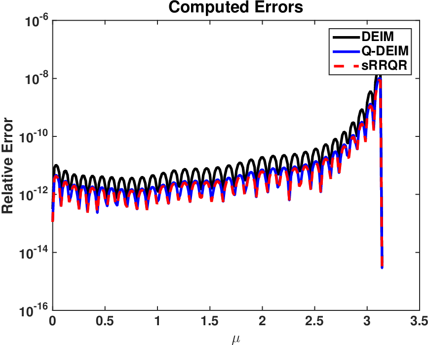

We observe that while all three methods are very accurate, Q–DEIM and sRRQR are much more accurate compared to DEIM for this example. Furthermore, from the right plot in Figure 2, we see that sRRQR is more accurate compared to both Q–DEIM and sRRQR. In practice, the performance of sRRQR is very similar to Q–DEIM, except for some adversarial cases in which Q–DEIM can fail spectacularly. In the subsequent examples, we use sRRQR for subset selection.
5.2 Example 2
Our next example is inspired by the Nonlinear RC-Ladder circuit, which is a standard benchmark problem for model reduction (see, for example [16, Section 6]). The underlying model is given by a dynamical system of the form
where and and . The diagonal matrix is chosen to have entries
The diagonal matrix induces the norm and the relative error between the full and the reduced order models are measured in this norm.
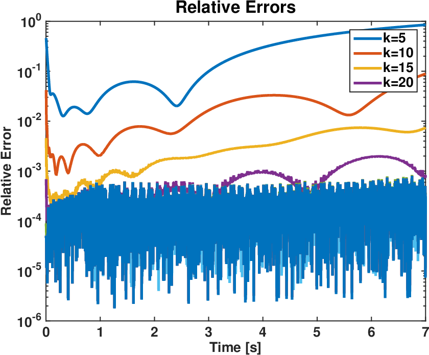
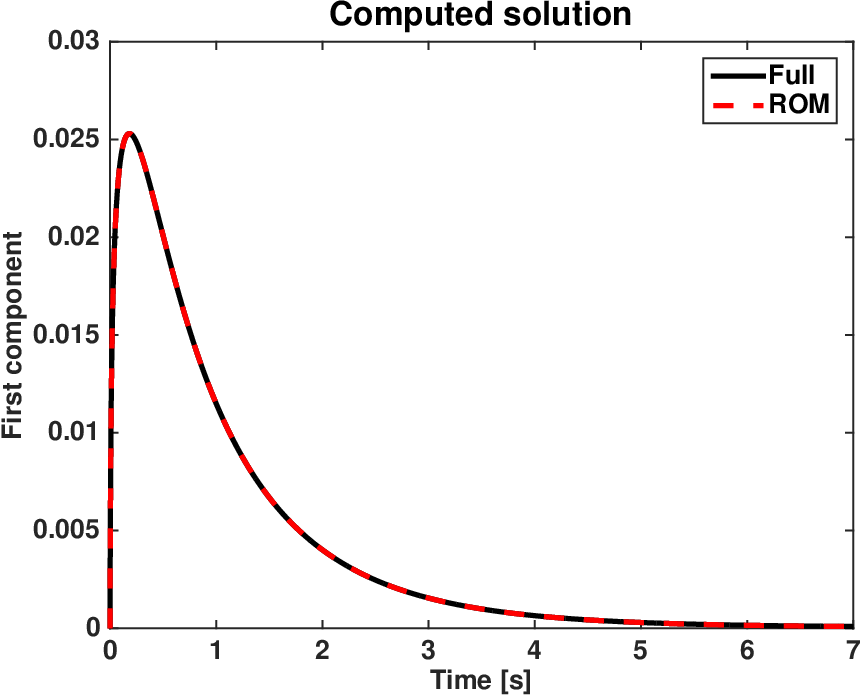
The dynamical system is simulated over seconds and snapshots of the dynamical system and the nonlinear function are collected with equidistant time steps. Based on the decay rate of the snapshots, we vary the number of basis vectors from to . The relative error is defined to be
where is the solution of the dynamical system at time , whereas is the reduced order approximation at the same time. The relative error as a function of number of retained basis vectors is plotted in left panel of Figure 3. On the right, the reconstruction of the first component of the dynamical system is shown; here basis vectors were retained. As can be seen, the reconstruction error is low and the -DEIM, indeed, approximates the large-scale dynamical system accurately.
5.3 Example 3
This example is inspired by [48, Section 2.3]. The spatial domain is taken to be and the parameter domain is . We define a function which satisfies
where . The function that is to be interpolated is
| (30) | |||||
| (31) |
Depending on the parameter , it has a sharp peak in one of the four corners of . The function is discretized on a grid in , and parameter samples are drawn from a equispaced grid in . These snapshots are used to construct the DEIM approximation. We choose three different weighting functions: is the identity matrix, is the weighting matrix corresponding to the inner product, and is the weighting matrix corresponding to the inner product.


We then compute the average relative error over a test sample corresponding to a equispaced grid in . The relative error is defined to be
The POD basis is computed using Algorithm 1, whereas the subset selection is done using sRRQR [25, Algorithm 4]. The results of the interpolation errors as a function of number of DEIM interpolation points retained, is displayed in the left panel of Figure 4. On the right hand panel of the same figure, we display the error constants . As can be seen, although the error constants increase with increasing number of basis vectors, the overall interpolation error decreases resulting an effective approximation.
5.4 Example 4
This is a continuation of Example 3. We use the same setup as before; however, we compare the different algorithms for -DEIM. In ‘Method 1’ we use Algorithm 1 to generate the POD basis, while the subset selection is done using sRRQR [25, Algorithm 4]. The error constant for this method is . In ‘Method 2’ we use Algorithm 2 with error constant and in ‘Method 3’ we use Algorithm 3 with error constant .
In Algorithm 2, the GSVD of the snapshot matrix w.r.t. the weighting matrix was computed as follows. First, the weighted QR was computed using [38, Algorithm 2] to obtain . Note that . Then the SVD of is computed as . We obtain the GSVD of , where now .


For a given weighting matrix, we define the relative error as
The DEIM operators correspond to the different Methods described above. In Figure 5 we plot the relative error using the DEIM approximation and error constants; here the weighting matrix corresponds to the inner product. As can be seen, the overall interpolation error from all three methods are comparable. However, the error constants for Method 2 are highest as expected, since it involves . In Figure 6 we repeat the same experiment; however, the weighting matrix corresponds to the inner product. Our conclusions are similar to the previous weighting matrix. Note here that is more ill-conditioned than and furthermore, for we have that . Therefore, the difference between the error constants for Methods 2 and 3 is very small.
In conclusion, for the application at hand, all three -DEIM methods produce comparable results. Methods 2 and 3 maybe desirable if factorization of is computationally expensive, or even infeasible.
5.5 Example 5
In this example, we consider a parameterized PDE based on [50, Section 8.5]. Consider the following parameterized PDE form defined on domain with boundary
| (32) | |||||
| (33) |
Here , and is the normal vector. The wind velocity is taken to be as , which is a constant in space but depends nonlinearly on the parameter . The source term has the form of a Gaussian function centered at and spread
The goal of this problem is to construct a reduced order model for the solution in the domain over the range of parameters , and . A POD based approach is used to reduce the model of the parameterized PDE with DEIM/WDEIM approximation for the source term.


As the weighting matrix , we choose the arising from the discrete representation of the inner product. For constructing the WPOD and WDEIM bases, we first generated a training set of parameters of points generated by Latin Hypercube sampling; then the source term and the solution of the PDE is computed at each training point . The maximum dimension for the WPOD and WDEIM bases were chosen to be and respectively based on the decay of the singular values. From the same snapshot set we also compute bases for the POD and DEIM with dimensions and respectively. For both approaches, we use the PQR for computing for point selections. We report the errors used by both approaches in Figure 7. The errors were averaged over different randomly generate samples in the parameter range. In the left panel, we compare the error in the DEIM approximation and WDEIM approximations of the source term , whereas in the right panel, we consider the error in the solution of over the same test samples. For the right panel, the dimension of the DEIM/W-DEIM was chosen to be and the dimension of the POD/WPOD basis dimension was chosen to be . All the errors were computed with the weighted norm . We see that the error in our approach (WPOD-WDEIM) is comparable with that of the POD-DEIM approach, whereas the error in the WDEIM approach is slightly better than the error in the error in the DEIM approach.
6 Conclusions
The main contributions of this work are: (i) it defines a new index selection operator, based on strong rank revealing QR factorization, that nearly attains the optimal DEIM projection error bound; (ii) it facilitates the understanding of the canonical structure of the DEIM projection; (iii) it establishes a core numerical linear algebra framework for the DEIM projection in weighted inner product spaces; (iv) it defines a discrete version of the Generalized Empirical Interpolation Method (GEIM). We believe that these will be useful for further development of the DEIM idea and its applications in scientific computing.
Acknowledgements
We are indebted to Ilse Ipsen and in particular to the two anonymous referees for constructive criticism and many suggestions that have improved the presentation of the paper.
References
- [1] David Amsallem and Jan Nordström, Energy stable model reduction of neurons by nonnegative discrete empirical interpolation, SIAM Journal on Scientific Computing, 38 (2016), pp. B297–B326.
- [2] E. Anderson, Z. Bai, C. Bischof, L. S. Blackford, J. Demmel, Jack J. Dongarra, J. Du Croz, S. Hammarling, A. Greenbaum, A. McKenney, and D. Sorensen, LAPACK Users’ Guide, Society for Industrial and Applied Mathematics (SIAM), Philadelphia, PA, third ed., 1999.
- [3] P. Astrid, S. Weiland, K. Willcox, and T. Backx, Missing point estimation in models described by proper orthogonal decomposition, IEEE Transactions on Automatic Control, 53 (2008), pp. 2237–2251.
- [4] M. F. Barone, I. Kalashnikova, D. J. Segalman, and H. K. Thornquist, Stable Galerkin reduced order models for linearized compressible flow, J. Comput. Phys., 228 (2009), pp. 1932–1946.
- [5] M. Barrault, N. C. Nguyen, Y. Maday, and A. T. Patera, An empirical interpolation method: Application to efficient reduced-basis discretization of partial differential equations, C. R. Acad. Sci. Paris, Série I., 339 (2004), pp. 667–672.
- [6] Peter Binev, Albert Cohen, Wolfgang Dahmen, Ronald DeVore, Guergana Petrova, and Przemyslaw Wojtaszczyk, Data assimilation in reduced modeling, SIAM/ASA Journal on Uncertainty Quantification, 5 (2017), pp. 1–29.
- [7] Å. Björck, Numerical Methods in Matrix Computations, Springer, Heidelberg, 2015.
- [8] Å. Björck and G. H. Golub, Numerical methods for computing angles between linear subspaces, Math. Comp., 27 (1973), pp. 579–594.
- [9] L. S. Blackford, J. Choi, A. Cleary, E. D’Azeuedo, J. Demmel, I. Dhillon, S. Hammarling, G. Henry, A. Petitet, K. Stanley, D. Walker, and R. C. Whaley, ScaLAPACK User’s Guide, Society for Industrial and Applied Mathematics (SIAM), Philadelphia, PA, 1997.
- [10] M. E. Broadbent, M. Brown, and K. Penner, Subset selection algorithms: Randomized vs. deterministic, SIAM Undergraduate Research Online, 3 (2010), pp. 50–71.
- [11] P. A. Businger and G. H. Golub, Linear least squares solutions by Householder transformations, Numer. Math., 7 (1965), pp. 269–276.
- [12] V. M. Calo, Y. Efendiev, J. Galvis, and M. Ghommem, Multiscale empirical interpolation for solving nonlinear PDEs, J. Comput. Phys., 278 (2014), pp. 204–220.
- [13] F. Casenave, A. Ern, and T. Lelièvre, Variants of the empirical interpolation method: Symmetric formulation, choice of norms and rectangular extension, Applied Mathematics Letters, 56 (2016), pp. 23–28.
- [14] S. Chandrasekaran and I. C. F. Ipsen, On rank-revealing QR factorisations, SIAM J. Matrix Anal. Appl., 15 (1994), pp. 592–622.
- [15] S. Chaturantabut and D. C. Sorensen, Nonlinear model reduction via discrete empirical interpolation, SIAM J. Sci. Comput., 32 (2010), pp. 2737–2764.
- [16] M. Condon and R. Ivanov, Empirical balanced truncation of nonlinear systems, J. Nonlinear Sci., 14 (2004), pp. 405–414.
- [17] F. Deutsch, Best approximation in inner product spaces, CMS books in mathematics/Ouvrages de Mathématiques de la SMC, 7, Springer Verlag, New York, 2001.
- [18] Z. Drmač and Z. Bujanović, On the failure of rank revealing QR factorization software – a case study, ACM Trans. Math. Softw., 35 (2008), pp. 1–28.
- [19] Z. Drmač and S. Gugercin, A new selection operator for the Discrete Empirical Interpolation Method – improved a priori error bound and extensions, SIAM J. Sci. Comput., 38 (2016), pp. A631–A648.
- [20] Charbel Farhat, Todd Chapman, and Philip Avery, Structure-preserving, stability, and accuracy properties of the energy-conserving sampling and weighting method for the hyper reduction of nonlinear finite element dynamic models, International Journal for Numerical Methods in Engineering, 102 (2015), pp. 1077–1110. nme.4820.
- [21] J. B. Freund and T. Colonius, POD analysis of sound generation by a turbulent jet, in 40th AIAA Aerospace Sciences Meeting, 2002.
- [22] G. H. Golub and C. F. Van Loan, Matrix Computations, Johns Hopkins University Press, Baltimore, MD, fourth ed., 2013.
- [23] S. A. Goreinov, E. E. Tyrtyshnikov, and N. L. Zamarashkin, A theory of pseudoskeleton approximations, Linear Algebra Appl., 261 (1997), pp. 1–21.
- [24] M.A. Grepl, Y. Maday, N.C. Nguyen, and A.T. Patera, Efficient reduced–basis treatment of nonaffine and nonlinear partial differential equations, ESAIM, Math. Model. Numer. Anal., 41 (2007), pp. 575–605.
- [25] M. Gu and S. C. Eisenstat, Efficient algorithms for computing a strong rank-revealing QR factorization, SIAM J. Sci. Comput., 17 (1996), pp. 848–869.
- [26] B. Haasdonk, M. Ohlberger, and G. Rozza, A reduced basis method for evolution schemes with parameter-dependent explicit operators, ETNA, 32 (2008), pp. 145–161.
- [27] P. Holmes, J.L. Lumley, G. Berkooz, and C.W. Rowley, Turbulence, Coherent Structures, Dynamical Systems and Symmetry, Cambridge Monographs on Mechanics, Cambridge University Press, 2014.
- [28] I. C. F. Ipsen, Numerical Matrix Analysis, Society for Industrial and Applied Mathematics (SIAM), Philadelphia, PA, 2009.
- [29] I. C. F. Ipsen and C. D. Meyer, The angle between complementary subspaces, Amer. Math. Monthly, 102 (1995), pp. 904–911.
- [30] W. Kahan, Numerical linear algebra, Canadian Mathematical Bulletin, 9 (1965), pp. 757–801.
- [31] I. Kalashnikova and S. Arunajatesan, A stable Galerkin reduced order modeling (ROM) for compressible flow, in 10th Wold Congress on Computational Mechanics, Blucher Mechanical Engineering Proceedings, May 2014.
- [32] I. Kalashnikova, S. Arunajatesan, M. F. Barone, B. G. van Bloemen Waanders, and J. A. Fike, Reduced order modeling for prediction and control of large–scale systems, Sandia Report SAND2014–4693, Sandia National Laboratories, May 2014.
- [33] I. Kalashnikova, M. F. Barone, S. Arunajatesan, and B. G. van Bloemen Waanders, Construction of energy-stable projection-based reduced order models, App. Math. Comput., 249 (2014), pp. 569–596.
- [34] D. E. Knuth, Semi-optimal bases for linear dependencies, Linear Multilinear Algebra, 17 (1985), pp. 1–4.
- [35] A. Kolmogoroff, Über die beste Annäherung von Funktionen einer gegebenen Funktionenklasse, Annals of Mathematics, 37 (1936), pp. 107–110.
- [36] M. A. Kowalski, K. A. Sikorski, and F. Stenger, Selected Topics in Approximation and Computation, Oxford University Press, 1995.
- [37] C.-J. Lin and R. Saigal, An incomplete Cholesky factorization for dense symmetric positive definite matrices, BIT, 40 (2000), pp. 536–558.
- [38] B. R. Lowery and J. Langou, Stability analysis of QR factorization in an oblique inner product, arXiv preprint arXiv:1401.5171, (2014).
- [39] Y. Maday and O. Mula, A generalized empirical interpolation method : Application of reduced basis techniques to data assimilation, in Analysis and Numerics of Partial Differential Equations, Springer INdAM Series, Springer, January 2013, pp. 221–235.
- [40] Y. Maday, O. Mula, A. T. Patera, and M. Yano, The generalized empirical interpolation method: Stability theory on Hilbert spaces with an application to the Stokes equation, Comput. Methods Appl. Mech. and Engrg., 287 (2015), pp. 310–334.
- [41] Y. Maday, O. Mula, and G. Turinici, Convergence analysis of the generalized empirical interpolation method, SIAM Journal on Numerical Analysis, 54 (2016), pp. 1713–1731.
- [42] Yvon Maday, Ngoc Cuong Nguyen, Anthony T. Patera, and S. H. Pau, A general multipurpose interpolation procedure: the magic points, Communications on Pure and Applied Analysis, 8 (2009), pp. 383–404.
- [43] Yvon Maday, Anthony T. Patera, James D. Penn, and Masayuki Yano, A parameterized-background data-weak approach to variational data assimilation: formulation, analysis, and application to acoustics, International Journal for Numerical Methods in Engineering, 102 (2015), pp. 933–965.
- [44] Maday, Yvon, T, Anthony, Penn, James D, and Yano, Masayuki, PBDW state estimation: Noisy observations; configuration-adaptive background spaces; physical interpretations, ESAIM: Proc., 50 (2015), pp. 144–168.
- [45] O. Mula, Some contributions towards the parallel simulation of time dependent neutron transport and the integration of observed data in real time, PhD thesis, Université Pierre et Marie Curie - Paris VI, November 2014. https://tel.archives-ouvertes.fr/tel-01081601.
- [46] F. Negri, A. Manzoni, and D. Amsallem, Efficient model reduction of parametrized systems by matrix discrete empirical interpolation, J. Comput. Phys., 303 (2015), pp. 431–454.
- [47] B. R. Noack, M. Schlegel, B. Ahlborn, G. Mutschke, M. Morzyński, P. Comte, and G. Tadmor, A finite-time thermodynamics of unsteady fluid flows, Journal of Non-Equilibrium Thermodynamics, 33 (2008), pp. 103–148.
- [48] B. Peherstorfer, D. Butnaru, K. Willcox, and H.-J. Bungartz, Localized discrete empirical interpolation method, SIAM J. Sci. Comput., 36 (2014), pp. A168–A192.
- [49] Benjamin Peherstorfer and Karen Willcox, Online adaptive model reduction for nonlinear systems via low-rank updates, SIAM Journal on Scientific Computing, 37 (2015), pp. A2123–A2150.
- [50] A. Quarteroni, A. Manzoni, and F. Negri, Reduced basis methods for partial differential equations: an introduction, vol. 92, Springer, 2015.
- [51] Satish C. Reddy, Peter J. Schmid, and Dan S. Henningson, Pseudospectra of the Orr–Sommerfeld operator, SIAM Journal on Applied Mathematics, 53 (1993), pp. 15–47.
- [52] C. W. Rowley, Model reduction for fluids, using balanced proper orthogonal decomposition, Internat. J. Bifur. Chaos Appl. Sci. Engrg., 15 (2005), pp. 997–1013.
- [53] C. W. Rowley, T. Colonius, and R. M. Murray, Model reduction for compressible flows using POD and Galerkin projection, Phys. D, 189 (2004), pp. 115–129.
- [54] G. Serre, P. Lafon, X. Gloerfelt, and C. Bailly, Reliable reduced-order models for time-dependent linearized Euler equations, J. Comput. Phys., 231 (2012), pp. 5176–5194.
- [55] G. W. Stewart, Computing the CS decomposition of a partitioned orthonormal matrix, Numer. Math., 40 (1982), pp. 297–306.
- [56] G. W. Stewart and Ji-Guang Sun, Matrix Perturbation Theory, Academic Press, 1990.
- [57] D. B. Szyld, The many proofs of an identity on the norm of oblique projections, Numer. Algorithms, 42 (2006), pp. 309–323.
- [58] M. Tabandeh and M. Wei, On the symmetrization in POD-Galerkin model for linearized compressible flows, in 54th AIAA Aerospace Sciences Meeting, 2016.
- [59] Paolo Tiso, Rob Dedden, and D.J. Rixen, A modified discrete empirical interpolation method for reducing non-linear structural finite element models, in International Design Engineering Technical Conferences & Computers and Information in Engineering Conference, no. 2013-13280, ASME, 4-7 August 2013.
- [60] Paolo Tiso and Daniel J. Rixen, Discrete Empirical Interpolation Method for Finite Element Structural Dynamics, Springer New York, New York, NY, 2013, pp. 203–212.
- [61] A. van der Sluis, Condition numbers and equilibration of matrices, Numer. Math., 14 (1969), pp. 14–23.
- [62] C. F. Van Loan, Generalizing the singular value decomposition, SIAM J. Numer. Anal., 13 (1976), pp. 76–83.
- [63] S. Volkwein, Model reduction using proper orthogonal decomposition, 2011. http://www.uni-graz. at/imawww/volkwein/POD.pdf.
- [64] P. Å Wedin, Perturbation bounds in connection with singular value decomposition, BIT Numerical Mathematics, 12 (1972), pp. 99–111.
- [65] P. Å. Wedin, On angles between subspaces of a finite dimensional inner product space, in Matrix Pencils, vol. 973 of Lecture Notes in Mathematics, Springer Verlag, 1982, pp. 263–285.
- [66] D. Wirtz, D. C. Sorensen, and B. Haasdonk, A posteriori error estimation for DEIM reduced nonlinear dynamical systems, SIAM Journal on Scientific Computing, 36 (2014), pp. A311–A338.
- [67] P. Zhu and A. V. Knyazev, Angles between subspaces and their tangents, J. Numer. Math., 21 (2013), pp. 325–340.
- [68] R. Zimmermann, A locally parametrized reduced-order model for the linear frequency domain approach to time-accurate computational fluid dynamics, SIAM Journal on Scientific Computing, 36 (2014), pp. B508–B537.
- [69] R. Zimmermann and S. Görtz, Non-linear reduced order models for steady aerodynamics, Procedia Computer Science, 1 (2010), pp. 165–174.
- [70] Ralf Zimmermann, Benjamin Peherstorfer, and Karen Willcox, Geometric subspace updates with applications to online adaptive nonlinear model reduction, ACDL Report TR15-3, Massachusetts Institute of Technology, Cambridge, MA, USA,, December 2015.
- [71] R. Zimmermann and K. Willcox, An accelerated greedy missing point estimation procedure, SIAM Journal on Scientific Computing, 38 (2016), pp. A2827–A2850.