跳到论文正文
W Papers独立论文阅读器 arXiv:1704.06550 论文正文 计算阅读时间 · 0%
引用这篇论文根据当前论文元数据生成,正式投稿前建议核对。


License: arXiv.org perpetual non-exclusive license
arXiv:1704.06550v1 [q-fin.MF] 21 Apr 2017

ON MEAN-VARIANCE HEDGING UNDER PARTIAL OBSERVATIONS AND TERMINAL WEALTH CONSTRAINTS

VITALII MAKOGIN Vitalii MakoginInstitute of Stochastics,
Ulm University, D-89069, Ulm, Germany
vitalii.makogin@uni-ulm.de
, ALEXANDER MELNIKOV Alexander MelnikovDepartment of Mathematical and Statistical Sciences,
University of Alberta, 632 Central Academic Building
Edmonton, AB T6G 2G1., Canada
melnikov@ualberta.ca
and YULIYA MISHURA Yuliya MishuraDepartment of Probability Theory, Statistics and Actuarial Mathematics,
Taras Shevchenko National University of Kyiv, Volodymyrska 64,
Kyiv, 01601, Ukraine
myus@univ.kiev.ua
Abstract.

In the paper a mean-square minimization problem under terminal wealth constraint with partial observations is studied. The problem is naturally connected to the mean-variance hedging problem under incomplete information. A new approach to solving this problem is proposed. The paper provides a solution when the underlying pricing process is a square-integrable semimartingale. The proposed method for study is based on the martingale representation. In special cases the Clark-Ocone representation can be used to obtain explicit solutions. The results and the method are illustrated and supported by example with two correlated geometric Brownian motions.

1. Introduction

Let us start with the problem which can arise on commodity markets. Particularly, the following example is given in the paper of [Weisshaupt (2003)]. Suppose that a mining company wants to exploit a certain mining area. The mineral AA which the mining company would produce after this investment is not traded now, but there exists another mineral A~\widetilde{A} with similar characteristics which is already traded on the market. Then the unobservable price process SS of the mineral AA is highly correlated with the price process S~\widetilde{S} of the mineral A~.\widetilde{A}. The mining company wants to insure against the risk that the price of the mineral AA after the period of investment TT will be below the production costs c.c. It invests money in options on mineral A~.\widetilde{A}. In this case, the company wants to find a strategy that minimizes the expected value of the squared difference between the price of AA and portfolio value. Such problem is called the problem of mean-variance hedging (MVH).

Since the pioneering work of [Föllmer & Sondermann (1986)], the mean-variance hedging is a permanent area of research in mathematical finance. At the beginning, the problem was formulated assuming that the probability measure was a martingale measure. In this context, some results were obtained in the case of full information by [Föllmer & Sondermann (1986)]. Under incomplete information this type of hedging was developed later in many papers. See, for example the paper of [Schweizer (1992)], where two correlated Wiener processes were considered and the hedging strategy could depend on both, and [Schweizer (1994)] where results were obtained using projection techniques.

We introduce the model of the present paper as follows. Assume that an agent used to work on well-known simple financial market and this market is observable enough to be complete. The agent wants to use financial instruments only from this market, and he wants to start working on a new unobservable market. We assume that this new market is incomplete. In our model there are two contingent claims H~\widetilde{H} and HH. The first one is observable and from the completeness of the observable market the agent superhedges H~\widetilde{H}, i.e., he chooses the strategy under which the terminal wealth exceeds the claim value. The second claim HH is from the new incomplete market and for reducing the new risk the agent uses the mean-variance approach, i.e., he simultaneously minimizes the mean-square difference of the terminal wealth and the unobservable claim. The simplest example of this model is the mean-variance hedging of unobservable claim HH using observable asset with the condition that portfolio value is non-negative at time T,T, i.e., in this case H~=0.\widetilde{H}=0. We assume that there are no arbitrage on both markets and therefore the value process of an admissible portfolio with non-negative terminal value is also non-negative. It enables us to consider the terminal constraint rather than the constraint which is pointwise in time.

To authors’ knowledge such an approach has not been considered in the existing literature. In the paper of [Föllmer & Leukert (2000)] the expectation of shortfall weighted by some loss function is minimized under condition that wealth process is non-negative on interval [0,T].[0,T]. In the paper of [Korn & Trautmann (1995)] investors trade in such a way that they achieve a non-negative wealth over the whole time interval [0,T].[0,T]. The authors’ analysis is based on the expected utility or the mean-variance approach and they gave a common framework including both types of selection criteria as special cases by considering portfolio problems with terminal wealth constraints. In the paper of [Korn (1997)] the considered problem is the mean-variance minimization for Black-Sholes model under condition that the terminal wealth only is non-negative. But author’s aim was concentrated on finding the terminal wealth value and the exact form of the minimization strategy was not given. In the paper of [Bielecki et al. (2005)] a continuous-time mean-variance portfolio selection problem is studied where all the market coefficients are random and the wealth process under any admissible trading strategy is not allowed to be below zero at any time.

In the paper [Fujii & Takahashi (2014)], the mean-variance hedging problem is studied in a partially observable market where the drift processes can only be inferred through the observation of asset or index processes. In the paper of [Ceci et al. (2014)] authors provide a suitable Galtchouk-Kunita-Watanabe decomposition of the contingent claim that works in a partial information framework. The paper [Hubalek et al. (2006)] considers variance-optimal hedging for processes with stationary independent increments. And in the paper of [Jeanblanc et al. (2012)] the problem of mean-variance hedging for general semimartingale models is solved via stochastic control methods.

Mathematically, the “unobservable” information is described by the filtration 𝔽={ℱt,t≥0}\mathbb{F}=\{\mathcal{F}_{t},t\geq 0\} and “observable” information is described by its subfiltration 𝔽~={ℱ~t,t≥0}.\widetilde{\mathbb{F}}=\{\widetilde{\mathcal{F}}_{t},t\geq 0\}. We restrict ourselves to the finite horizon T>0.T>0. The prices of underlying asset are given by 𝔽~\widetilde{\mathbb{F}}-adapted square-integrable stochastic process S~={S~t,t∈[0,T]}.\widetilde{S}=\{\widetilde{S}_{t},t\in[0,T]\}. We assume that S~\widetilde{S} be a semimartingale. A trading strategy is described by 𝔽~\widetilde{\mathbb{F}}-predictable square-integrable stochastic processes ξ={ξt,t∈[0,T]}\xi=\{\xi_{t},t\in[0,T]\} such that the stochastic integral ∫0Tξt​d​S~t\int_{0}^{T}\xi_{t}d\widetilde{S}_{t} is well-defined. This integral describes the trading gains induced by the self-financing portfolio strategy associated to ξ.\xi. Let a contingent claim H~\widetilde{H} be a ℱ~T\widetilde{\mathcal{F}}_{T}-measurable square-integrable nonnegative random variable. At time TT, a hedger who starts with initial capital xx and uses the strategy ξ,\xi, has to pay the random amount H~,\widetilde{H}, so that portfolio value should not be less than H~.\widetilde{H}. This contingent claim H~\widetilde{H} can be interpreted as a random lower bound on a terminal wealth. At the same time hedger wants to approximate a random amount HH by portfolio value. In contradiction to H~\widetilde{H}, we assume that HH is a ℱT\mathcal{F}_{T}-measurable square-integrable non-negative random variable. In this context, mean-variance hedging problem with partial observations means solving the optimization problem

minimize ​𝔼​(H−x−∫0Tξt​d​S~t)2​ over all ​ξ∈Ξ⁡(x,H~),\mbox{minimize }\mathbb{E}\left(H-x-\int_{0}^{T}\xi_{t}d\widetilde{S}_{t}\right)^{2}\mbox{ over all }\xi\in\Xi(x,\widetilde{H}),

where Ξ(x,H~)={ξ:x+∫0TξtdS~t≥H~a.s.}\Xi(x,\widetilde{H})=\{\xi:x+\int_{0}^{T}\xi_{t}d\widetilde{S}_{t}\geq\widetilde{H}~a.s.\}

This problem is naturally related to the mean-variance hedging. The main challenge in solving mean-variance hedging problem is to find more explicit descriptions of the optimal strategy and in the present paper we introduce the new approach. The concrete form of the minimizing strategy can be obtained by the Clark-Ocone formula when it is applicable.

We consider the example of this problem when pricing processes of observable and unobservable assets S~\widetilde{S}, SS are two correlated geometric Wiener processes. In this case we can use the delta-hedging but we illustrate how our method works by applying the Clark-Ocone theorem in the Brownian setting. For the case when the contingent claim HH is a call-option we provide the precise formula of the solution and make numerical illustrations.

The paper is organized as follows. In section 2 we formulate the conditional mean-variance hedging problem under incomplete information in the general semimartingale setting. In section 3 we reduce it to the simplified statement in order to avoid technical details. We prove the auxiliary result concerning the representation of the random variable that is approached and prove the main result that gives the solution of the minimization problem. In section 4 the corresponding results are illustrated with the help of the model with two correlated geometric Wiener processes. In subsection 4.1 we present the numerical illustrations.

2. Preliminaries and the Formulation of a Problem

Let we have complete probability space (Ω,ℱ,P)(\Omega,\mathcal{F},P) with filtration 𝔽={ℱt,t≥0}\mathbb{F}=\{\mathcal{F}_{t},t\geq 0\} that corresponds to the “complete information”. Suppose that there exists a subfiltration 𝔽~={ℱ~t,t≥0}\mathbb{\widetilde{F}}=\{\widetilde{\mathcal{F}}_{t},t\geq 0\} that corresponds to the “incomplete information”. Consider càdlàg risk asset S~={St~,t≥0}\widetilde{S}=\{\widetilde{S_{t}},t\geq 0\} such that S~\widetilde{S} is non-negative and adapted to the “incomplete information”, or, that is the same for us, 𝔽~\mathbb{\widetilde{F}}-adapted. We suppose that non-risky asset Bt≡1B_{t}\equiv 1 and the market Σ\Sigma is arbitrage-free on (Ω,ℱ,P)(\Omega,\mathcal{F},P) with filtration 𝔽\mathbb{F}. Moreover, we suppose that S~∈Σ\widetilde{S}\in\Sigma and the observable market Σ~={1,S~}\widetilde{\Sigma}={\{1,\widetilde{S}\}} is complete on (Ω,ℱ,P)(\Omega,\mathcal{F},P) with filtration 𝔽~⊂𝔽\mathbb{\widetilde{F}}\subset\mathbb{F}. We restrict ourselves to the finite horizon TT, so we consider all processes on the interval [0,T][0,T]. Let 𝒫\mathcal{P} be the set of all equivalent martingale measures for Σ\Sigma. Then the restriction P~\widetilde{P} of any P∗∈𝒫P^{*}\in\mathcal{P} on 𝔽~\mathbb{\widetilde{F}} is the same unique equivalent martingale measure for the observable market Σ~\widetilde{\Sigma} so that S~\widetilde{S} is 𝔽~\mathbb{\widetilde{F}}-martingale w.r.t. P~.\widetilde{P}. Denote DT=d​P~Td​PTD_{T}=\frac{d\widetilde{P}_{T}}{dP_{T}} the restriction of d​P~d​P\frac{d\widetilde{P}}{dP} on interval [0,T][0,T].

Now we introduce two square-integrable nonnegative random variables, HH and H~\widetilde{H}, HH being ℱT{\mathcal{F}}_{T}-measurable and H~\widetilde{H} being ℱ~T\widetilde{\mathcal{F}}_{T}-measurable. We can characterize them as “unobservable” and “observable” random variables or contingent claims, correspondingly.

In order to remain within the framework of the square-integrable approach, we introduce the following assumptions.

  1. (A​1)(A1)

    S~={St~,t≥0}\widetilde{S}=\{\widetilde{S_{t}},t\geq 0\} is the semimartingale admitting the representation St~=Nt~+At~,\widetilde{S_{t}}=\widetilde{N_{t}}+\widetilde{A_{t}}, where N~\widetilde{N} is the square-integrable martingale and A~\widetilde{A} is the predictable process of square-integrable variation. Suppose that 𝔽~\mathbb{\widetilde{F}} is generated by N~={N~t,t≥0}\widetilde{N}=\{\widetilde{N}_{t},t\geq 0\}.

  2. (A​2)(A2)

    𝔼​DT2<∞,\mathbb{E}D_{T}^{2}<\infty, 𝔼​H2<∞\mathbb{E}H^{2}<\infty and 𝔼​H~2<∞.\mathbb{E}\widetilde{H}^{2}<\infty.

These conditions mean, in particular, that we can consider stochastic integral w.r.t. the semimartingale S~,\widetilde{S},

I⁡(t,ξ)=∫0tξs​d​S~s=∫0tξs​d​N~s+∫0tξs​d​A~s,t∈[0,T]{I}(t,{\xi})=\int_{0}^{t}\xi_{s}d\widetilde{S}_{s}=\int_{0}^{t}\xi_{s}d\widetilde{N}_{s}+\int_{0}^{t}\xi_{s}d\widetilde{A}_{s},\;t\in[0,T]

for such 𝔽~\mathbb{\widetilde{F}}-predictable processes ξ\xi that ∫0Tξs2​d​⟨N~⟩s<∞\int_{0}^{T}\xi_{s}^{2}d\langle\widetilde{N}\rangle_{s}<\infty and ∫0T|ξs|​d​|A~|s<∞\int_{0}^{T}|\xi_{s}|d|\widetilde{A}|_{s}<\infty a.s.

Denote Ξ\Xi class of such 𝔽~\mathbb{\widetilde{F}}-predictable strategies.

Completeness of market Σ~\widetilde{\Sigma} together with condition (A​2)(A2) means that for any initial value x≥𝔼P~​H~x\geq\mathbb{E}_{\widetilde{P}}\widetilde{H} we can construct the superhedge of the contingent claim H~\widetilde{H} a.s. with the help of such ξ∈Ξ\xi\in\Xi that 𝔼​(I⁡(T,ξ))2<∞\mathbb{E}({I}(T,{\xi}))^{2}<\infty. In other words, there exists such ξ∈Ξ\xi\in\Xi that x+I⁡(T,ξ)≥H~a.s.x+{I}(T,{\xi})\geq\widetilde{H}\quad a.s. Further, for any x∈ℝx\in\mathbb{R} denote

Ξ⁡(x,H~)={ξ∈Ξ:x+∫0Tξs​d​S~s≥H~​a.s.}.\Xi(x,\widetilde{H})=\{\xi\in\Xi:x+\int_{0}^{T}\xi_{s}d\widetilde{S}_{s}\geq\widetilde{H}\;\textit{a.s.}\}.

Note, if x<𝔼P~​H~,x<\mathbb{E}_{\widetilde{P}}\widetilde{H}, then the space of admissible strategies is empty. So, in what follows, we can assume that x≥𝔼P~​H~.x\geq\mathbb{E}_{\widetilde{P}}\widetilde{H}.

Now we can state a conditional minimization problem in the semimartingale framework.

Problem [S⁡(x,H~,H)][S({x,{\widetilde{H}};{H}})]. Starting with fixed value x≥𝔼P~​H~,x\geq\mathbb{E}_{\widetilde{P}}\widetilde{H}, to construct the hedging strategy ξ~∈Ξ⁡(x,H~)\widetilde{\xi}\in\Xi(x,\widetilde{H}) so that

𝔼​(H−x−∫0Tξ~s​d​S~s)2=minξ∈Ξ⁡(x,H~)⁡𝔼​(H−x−∫0Tξs​d​S~s)2,\mathbb{E}\left(H-x-\int_{0}^{T}\widetilde{\xi}_{s}d\widetilde{S}_{s}\right)^{2}=\min_{\xi\in\Xi(x,\widetilde{H})}\mathbb{E}\left(H-x-\int_{0}^{T}\xi_{s}d\widetilde{S}_{s}\right)^{2},

and such ξ~\widetilde{\xi} for which

minξ∈Ξ⁡(x,H~)⁡𝔼​(H−x−∫0Tξs​d​S~s)2=𝔼​(H−x−∫0Tξ~s​d​S~s)2.\min_{\xi\in\Xi(x,\widetilde{H})}\mathbb{E}\left({H}-x-\int_{0}^{T}\xi_{s}d\widetilde{S}_{s}\right)^{2}=\mathbb{E}\left({H}-x-\int_{0}^{T}\widetilde{\xi}_{s}d\widetilde{S}_{s}\right)^{2}.

Note that if N~\widetilde{N} has a martingale representation property then the the market Σ~\widetilde{\Sigma} is complete. For example, Brownian motion and compensated Poisson process have this property.

3. Main results

In order to simplify the solving of Problem [S⁡(x,H~,H)][S({x,{\widetilde{H}};{H}})] we make the following remarks.

Remark 3.1.

We present 𝔼​(H−x−∫0Tξs​d​S~s)2\mathbb{E}\left(H-x-\int_{0}^{T}\xi_{s}d\widetilde{S}_{s}\right)^{2} as

𝔼​(H−𝔼⁡(H|ℱ~T)+𝔼⁡(H|ℱ~T)−x−∫0Tξs​d​S~s)2\displaystyle\mathbb{E}\left(H-\mathbb{E}(H|\widetilde{\mathcal{F}}_{T})+\mathbb{E}(H|\widetilde{\mathcal{F}}_{T})-x-\int_{0}^{T}\xi_{s}d\widetilde{S}_{s}\right)^{2}
=𝔼​(H−𝔼⁡(H|ℱ~T))2+𝔼​(𝔼⁡(H|ℱ~T)−x−∫0Tξs​d​S~s)2,\displaystyle=\mathbb{E}\left(H-\mathbb{E}(H|\widetilde{\mathcal{F}}_{T})\right)^{2}+\mathbb{E}\left(\mathbb{E}(H|\widetilde{\mathcal{F}}_{T})-x-\int_{0}^{T}\xi_{s}d\widetilde{S}_{s}\right)^{2},

since H−𝔼⁡(H|ℱ~T)H-\mathbb{E}(H|\widetilde{\mathcal{F}}_{T}) and any square-integrable ℱ~T\widetilde{\mathcal{F}}_{T}-measurable random variable are orthogonal. So, Problem [S⁡(x,H~,H)][S({x,{\widetilde{H}};{H}})] is reduced to the finding of

(3.1) minξ∈Ξ⁡(x,H~)⁡𝔼​(𝔼⁡(H|ℱ~T)−x−∫0Tξs​d​S~s)2,\begin{gathered}\min_{\xi\in\Xi(x,\widetilde{H})}\mathbb{E}\left(\mathbb{E}(H|\widetilde{\mathcal{F}}_{T})-x-\int_{0}^{T}\xi_{s}d\widetilde{S}_{s}\right)^{2},\end{gathered}

and such ξ~\widetilde{\xi} for which

minξ∈Ξ⁡(x,H~)⁡𝔼​(𝔼⁡(H|ℱ~T)−x−∫0Tξs​d​S~s)2=𝔼​(𝔼⁡(H|ℱ~T)−x−∫0Tξ~s​d​S~s)2.\min_{\xi\in\Xi(x,\widetilde{H})}\mathbb{E}\left(\mathbb{E}(H|\widetilde{\mathcal{F}}_{T})-x-\int_{0}^{T}\xi_{s}d\widetilde{S}_{s}\right)^{2}=\mathbb{E}\left(\mathbb{E}(H|\widetilde{\mathcal{F}}_{T})-x-\int_{0}^{T}\widetilde{\xi}_{s}d\widetilde{S}_{s}\right)^{2}.
Remark 3.2.

Denote H1=𝔼⁡(H|ℱ~T).H_{1}=\mathbb{E}(H|\widetilde{\mathcal{F}}_{T}). Consider the expansion H1=H1​𝟙H1≥H~+H1​𝟙H1<H~H_{1}=H_{1}\mathbbm{1}_{H_{1}\geq\widetilde{H}}+H_{1}\mathbbm{1}_{H_{1}<\widetilde{H}} and denote H2=H1​𝟙H1≥H~+H~​𝟙H1<H~≥H~H_{2}=H_{1}\mathbbm{1}_{H_{1}\geq\widetilde{H}}+\widetilde{H}\mathbbm{1}_{H_{1}<\widetilde{H}}\geq\widetilde{H}. On one hand, for any ξ∈Ξ⁡(x,H~)\xi\in\Xi(x,\widetilde{H})

𝔼​(H1−x−∫0Tξs​d​S~s)2\displaystyle\mathbb{E}\left(H_{1}-x-\int_{0}^{T}\xi_{s}d\widetilde{S}_{s}\right)^{2}
=𝔼​(H1−x−∫0Tξs​d​S~s)2​𝟙H1<H~+𝔼​(H1−x−∫0Tξs​d​S~s)2​𝟙H1≥H~\displaystyle=\mathbb{E}\left(H_{1}-x-\int_{0}^{T}\xi_{s}d\widetilde{S}_{s}\right)^{2}\mathbbm{1}_{H_{1}<\widetilde{H}}+\mathbb{E}\left(H_{1}-x-\int_{0}^{T}\xi_{s}d\widetilde{S}_{s}\right)^{2}\mathbbm{1}_{H_{1}\geq\widetilde{H}}
(3.2) ≥𝔼​(H~−x−∫0Tξs​d​S~s)2​𝟙H1<H~+𝔼​(H1−x−∫0Tξs​d​S~s)2​𝟙H1≥H~\displaystyle\geq\mathbb{E}\left(\widetilde{H}-x-\int_{0}^{T}\xi_{s}d\widetilde{S}_{s}\right)^{2}\mathbbm{1}_{H_{1}<\widetilde{H}}+\mathbb{E}\left(H_{1}-x-\int_{0}^{T}\xi_{s}d\widetilde{S}_{s}\right)^{2}\mathbbm{1}_{H_{1}\geq\widetilde{H}}
=𝔼​(H2−x−∫0Tξs​d​S~s)2.\displaystyle=\mathbb{E}\left(H_{2}-x-\int_{0}^{T}\xi_{s}d\widetilde{S}_{s}\right)^{2}.

On the other hand, for any ξ∈Ξ⁡(x,H~)\xi\in\Xi(x,\widetilde{H})

𝔼​(H1−x−∫0Tξs​d​S~s)2=𝔼​(H1​𝟙H1≥H~+H1​𝟙H1<H~−x−∫0Tξs​d​S~s)2\displaystyle\mathbb{E}\left(H_{1}-x-\int_{0}^{T}\xi_{s}d\widetilde{S}_{s}\right)^{2}=\mathbb{E}\left(H_{1}\mathbbm{1}_{H_{1}\geq\widetilde{H}}+H_{1}\mathbbm{1}_{H_{1}<\widetilde{H}}-x-\int_{0}^{T}\xi_{s}d\widetilde{S}_{s}\right)^{2}
=𝔼​(H1​𝟙H1≥H~−x−∫0Tξs​d​S~s)2+𝔼​(H1​𝟙H1<H~)2\displaystyle=\mathbb{E}\left(H_{1}\mathbbm{1}_{H_{1}\geq\widetilde{H}}-x-\int_{0}^{T}\xi_{s}d\widetilde{S}_{s}\right)^{2}+\mathbb{E}\left(H_{1}\mathbbm{1}_{H_{1}<\widetilde{H}}\right)^{2}
−2​𝔼​(x+∫0Tξs​d​S~s)​H1​𝟙H1<H~\displaystyle-2\mathbb{E}\left(x+\int_{0}^{T}\xi_{s}d\widetilde{S}_{s}\right)H_{1}\mathbbm{1}_{H_{1}<\widetilde{H}}
≤𝔼​(H1​𝟙H1≥H~−x−∫0Tξs​d​S~s)2+𝔼​(H1​𝟙H1<H~)2−2​𝔼​(H~​H1​𝟙H1<H~)\displaystyle\leq\mathbb{E}\left(H_{1}\mathbbm{1}_{H_{1}\geq\widetilde{H}}-x-\int_{0}^{T}\xi_{s}d\widetilde{S}_{s}\right)^{2}+\mathbb{E}\left(H_{1}\mathbbm{1}_{H_{1}<\widetilde{H}}\right)^{2}-2\mathbb{E}\left(\widetilde{H}H_{1}\mathbbm{1}_{H_{1}<\widetilde{H}}\right)
(3.3) ≤𝔼​(H1​𝟙H1≥H~−x−∫0Tξs​d​S~s)2−𝔼​(H1​𝟙H1<H~)2,\displaystyle\leq\mathbb{E}\left(H_{1}\mathbbm{1}_{H_{1}\geq\widetilde{H}}-x-\int_{0}^{T}\xi_{s}d\widetilde{S}_{s}\right)^{2}-\mathbb{E}\left(H_{1}\mathbbm{1}_{H_{1}<\widetilde{H}}\right)^{2},

and the equalities in (3.2),(3.3) are achieved if and only if H1≥H~H_{1}\geq\widetilde{H} a.s. Therefore, we can restrict ourselves to the case H1≥H~H_{1}\geq\widetilde{H} a.s. and in other cases apply bounds (3.2),(3.3) (It will be specified in Remark 3.5 how to deal with the upper bound in (3.3).)

Remark 3.3.

Now, let H1≥H~H_{1}\geq\widetilde{H} a.s. and consider the case when x=𝔼P~​H1.x=\mathbb{E}_{\widetilde{P}}H_{1}. It follows from the completeness of the market Σ~\widetilde{\Sigma} that we have the representation H1=x+∫0Tξs0​d​S~sH_{1}=x+\int_{0}^{T}\xi^{0}_{s}d\widetilde{S}_{s} for some ξ0∈Ξ⁡(x,H~)\xi^{0}\in\Xi(x,\widetilde{H}). So, we put ξ~=ξ0\widetilde{\xi}=\xi^{0} and get the trivial zero solution of minimization problem. So, it is reasonable to consider two cases: x<𝔼P~​H1x<\mathbb{E}_{\widetilde{P}}H_{1} and x>𝔼P~​H1x>\mathbb{E}_{\widetilde{P}}H_{1}. However, since our goal is to solve the minimization problem with minimal initial resources, we suppose in what follows that x<𝔼P~​H1x<\mathbb{E}_{\widetilde{P}}H_{1}.

Remark 3.4.

Further, let 𝔼P~​H~≤x<𝔼P~​H1\mathbb{E}_{\widetilde{P}}\widetilde{H}\leq x<\mathbb{E}_{\widetilde{P}}H_{1}. Evidently, 𝔼​(H1−x−∫0Tξs​d​S~s)2\mathbb{E}\left(H_{1}-x-\int_{0}^{T}\xi_{s}d\widetilde{S}_{s}\right)^{2} =𝔼​(H1−H~−(x+∫0Tξs​d​S~s−H~))2.=\mathbb{E}\left(H_{1}-\widetilde{H}-\left(x+\int_{0}^{T}\xi_{s}d\widetilde{S}_{s}-\widetilde{H}\right)\right)^{2}. It follows from the completeness of the market that there exists η∈Ξ{\eta}\in\Xi such that H~=𝔼P~​H~+∫0Tηs​d​S~s.\widetilde{H}=\mathbb{E}_{\widetilde{P}}\widetilde{H}+\int_{0}^{T}{\eta}_{s}d\widetilde{S}_{s}. Now, rewrite

𝔼​(H1−x−∫0Tξs​d​S~s)2=𝔼​(H1−H~−(x−𝔼P~​H~+∫0T(ξs−ηs)​d​S~s))2,\mathbb{E}\left(H_{1}-x-\int_{0}^{T}\xi_{s}d\widetilde{S}_{s}\right)^{2}=\mathbb{E}\left(H_{1}-\widetilde{H}-\left(x-\mathbb{E}_{\widetilde{P}}\widetilde{H}+\int_{0}^{T}(\xi_{s}-\eta_{s})d\widetilde{S}_{s}\right)\right)^{2},

denote G=H1−H~G=H_{1}-\widetilde{H}, g=x−x~g=x-\widetilde{x}, ζs=ξs−ηs,{\zeta}_{s}=\xi_{s}-\eta_{s}, and note that G≥0G\geq 0 a.s., 𝔼​G>0\mathbb{E}G>0. Then obviously 0≤g<𝔼P~​G0\leq g<\mathbb{E}_{\widetilde{P}}G and g+∫0Tζs​d​S~s=x−x~+∫0T(ξs−ηs)​d​S~s≥H~−H~=0g+\int_{0}^{T}\zeta_{s}d\widetilde{S}_{s}=x-\widetilde{x}+\int_{0}^{T}(\xi_{s}-\eta_{s})d\widetilde{S}_{s}\geq\widetilde{H}-\widetilde{H}=0 a.s. The case g=0g=0 corresponds to x=𝔼P~​H~x=\mathbb{E}_{\widetilde{P}}\widetilde{H} and then the trivial solution of [S⁡(x,H~,H)][S({x,{\widetilde{H}};{H}})] is the strategy ηs.{\eta}_{s}. So, further we assume g>0g>0 or x>𝔼P~​H~.x>\mathbb{E}_{\widetilde{P}}\widetilde{H}. It means that we reduce Problem [S⁡(x,H~,H)][S({x,{\widetilde{H}};{H}})] to the following one.

Problem [S⁡(g,0,G)][S({g,0;{G}})]. For fixed square-integrable nonnegative F~T{\widetilde{F}}_{T}-measurable random variable GG and fixed number 0<g<𝔼P~​G0<g<\mathbb{E}_{\widetilde{P}}G to find

minξ∈Ξ⁡(g,0)⁡𝔼​(G−g−∫0Tξs​d​S~s)2,\min_{\xi\in\Xi(g,0)}\mathbb{E}\left(G-g-\int_{0}^{T}\xi_{s}d\widetilde{S}_{s}\right)^{2},

and such ξ~∈Ξ⁡(g,0)\widetilde{\xi}\in\Xi(g,0) for which

minξ∈Ξ⁡(g,0)⁡𝔼​(G−g−∫0Tξs​d​S~s)2=𝔼​(G−g−∫0Tξ~s​d​S~s)2.\min_{\xi\in\Xi(g,0)}\mathbb{E}\left(G-g-\int_{0}^{T}\xi_{s}d\widetilde{S}_{s}\right)^{2}=\mathbb{E}\left(G-g-\int_{0}^{T}\widetilde{\xi}_{s}d\widetilde{S}_{s}\right)^{2}.
Remark 3.5.

Consider the term 𝔼⁡(x,S~):=𝔼​(H1​𝟙H1≥H~−x−∫0Tξs​d​S~s)2\mathbb{E}(x,\widetilde{S}):=\mathbb{E}\left(H_{1}\mathbbm{1}_{H_{1}\geq\widetilde{H}}-x-\int_{0}^{T}\xi_{s}d\widetilde{S}_{s}\right)^{2} from (3.3). We can present it as

𝔼⁡(x,S~)=𝔼​((H1−H~)​𝟙H1≥H~−(x+∫0Tξs​d​S~s−H~​𝟙H1≥H~))2.\mathbb{E}(x,\widetilde{S})=\mathbb{E}\left((H_{1}-\widetilde{H})\mathbbm{1}_{H_{1}\geq\widetilde{H}}-\left(x+\int_{0}^{T}\xi_{s}d\widetilde{S}_{s}-\widetilde{H}\mathbbm{1}_{H_{1}\geq\widetilde{H}}\right)\right)^{2}.

It follows from the market completeness that H~​𝟙H1≥H~\widetilde{H}\mathbbm{1}_{H_{1}\geq\widetilde{H}} admits the representation

H~​𝟙H1≥H~=x~1+∫0Tγ~s​d​S~s,\widetilde{H}\mathbbm{1}_{H_{1}\geq\widetilde{H}}=\widetilde{x}_{1}+\int_{0}^{T}\widetilde{\gamma}_{s}d\widetilde{S}_{s},

where x~1=𝔼P~​H~​𝟙H1≥H~≤𝔼P~​H~≤x\widetilde{x}_{1}=\mathbb{E}_{\widetilde{P}}\widetilde{H}\mathbbm{1}_{H_{1}\geq\widetilde{H}}\leq\mathbb{E}_{\widetilde{P}}\widetilde{H}\leq x and x+∫0Tξs​d​S~s−H~​𝟙H1≥H~≥0x+\int_{0}^{T}\xi_{s}d\widetilde{S}_{s}-\widetilde{H}\mathbbm{1}_{H_{1}\geq\widetilde{H}}\geq 0. Therefore, the minimization of the term 𝔼⁡(x,S~)\mathbb{E}(x,\widetilde{S}) is in the framework of the Problem [S⁡(g,0,G)][S({g,0;{G}})] with g=x−x~1≥0g=x-\widetilde{x}_{1}\geq 0 and G=(H1−H~)​𝟙H1≥H~≥0G=(H_{1}-\widetilde{H})\mathbbm{1}_{H_{1}\geq\widetilde{H}}\geq 0. So, in the general case, when the inequality H1≥H~H_{1}\geq\widetilde{H} does not hold a.s., we can minimize right-hand side of (3.3) in the framework of the Problem [S⁡(g,0,G)][S({g,0;{G}})] and find the minimization strategy ξ~t.\widetilde{\xi}_{t}. The minimum value minξ∈Ξ⁡(x,H~)⁡𝔼​(𝔼⁡(H|ℱ~T)−x−∫0Tξs​d​S~s)2\min_{\xi\in\Xi(x,\widetilde{H})}\mathbb{E}\left(\mathbb{E}(H|\widetilde{\mathcal{F}}_{T})-x-\int_{0}^{T}\xi_{s}d\widetilde{S}_{s}\right)^{2} will be between the right-hand side of (3.2) evaluated for strategy ξ~t+γ~t\widetilde{\xi}_{t}+\widetilde{\gamma}_{t} and the minimum value of the right-hand side of (3.3).

To solve Problem [S⁡(g,0,G)][S({g,0;{G}})], recall DT=d​P~Td​PTD_{T}=\frac{d\widetilde{P}_{T}}{dP_{T}} is the restriction of d​P~d​P\frac{d\widetilde{P}}{dP} on [0,T][0,T] and note that for any v⁡(x)∈ℝv(x)\in\mathbb{R}

𝔼P~​(G+v⁡(x)​DT)+≤𝔼​DT​G+|v⁡(x)|​𝔼​DT2<+∞.\mathbb{E}_{\widetilde{P}}\left(G+v(x)D_{T}\right)^{+}\leq\mathbb{E}D_{T}G+|v(x)|\mathbb{E}D^{2}_{T}<+\infty.

Now, for any 0<x<𝔼P~​G0<x<\mathbb{E}_{\widetilde{P}}G consider v⁡(x)v(x) that is the solution of equation

(3.4) 𝔼P~​(G+v⁡(x)​DT)+=x.\mathbb{E}_{\widetilde{P}}\left(G+v(x)D_{T}\right)^{+}=x.

We see that v⁡(x)v(x) is non decreasing.

Lemma 3.6.

Function v=v⁡(x),x∈(0,𝔼P~​G)v=v(x),\;x\in(0,\mathbb{E}_{\widetilde{P}}G) is uniquely determined, continuous and strictly increasing on the interval (0,𝔼P~​G)(0,\mathbb{E}_{\widetilde{P}}G). The range of values of this function is the interval (r,0)(r,0), where r=−esssupω∈ΩG/DT.r=-{\mathrm{ess}\sup}_{\omega\in\Omega}G/D_{T}.

Proof.

Evidently, function f⁡(y)=𝔼P~​(y​DT+G)+f(y)=\mathbb{E}_{\widetilde{P}}\left(yD_{T}+G\right)^{+} is non-decreasing and continuous on ℝ\mathbb{R}, limy→−∞f⁡(y)=0\lim_{y\rightarrow-\infty}f(y)=0 and limy→+∞f⁡(y)=+∞\lim_{y\rightarrow+\infty}f(y)=+\infty. Therefore, for any x∈(0,𝔼P~​G)x\in(0,\mathbb{E}_{\widetilde{P}}G) solution of equation (3.4) exists. Furthermore, let for y1<y2y_{1}<y_{2}

(3.5) 𝔼P~​(y1​DT+G)+=𝔼P~​(y2​DT+G)+=x>0.\mathbb{E}_{\widetilde{P}}\left(y_{1}D_{T}+G\right)^{+}=\mathbb{E}_{\widetilde{P}}\left(y_{2}D_{T}+G\right)^{+}=x>0.

Then P~{G>−y1DT}>0\widetilde{P}\{G>-y_{1}D_{T}\}>0 therefore with positive probability (y2​DT+G)+>\left(y_{2}D_{T}+G\right)^{+}> (y1​DT+G)+\left(y_{1}D_{T}+G\right)^{+} that is in contradiction with (3.5). Therefore, solution of equation (3.4) is unique and function v=v⁡(x),v∈(0,𝔼P~​G)v=v(x),v\in(0,\mathbb{E}_{\widetilde{P}}G) is uniquely determined. Now, 𝔼P~​(v⁡(x)​DT+G)+\mathbb{E}_{\widetilde{P}}\left(v(x)D_{T}+G\right)^{+} strictly increases in x∈(0,𝔼P~​G)x\in(0,\mathbb{E}_{\widetilde{P}}G). Indeed, let 𝔼P~​G>x2>x1>0\mathbb{E}_{\widetilde{P}}G>x_{2}>x_{1}>0 and

𝔼P~​(v⁡(x2)​DT+G)+=x2>𝔼P~​(v⁡(x1)​DT+G)+=x1>0.\mathbb{E}_{\widetilde{P}}\left(v(x_{2})D_{T}+G\right)^{+}=x_{2}>\mathbb{E}_{\widetilde{P}}\left(v(x_{1})D_{T}+G\right)^{+}=x_{1}>0.

It means in particular that

𝟙{v(x2)DT+G>0}−𝟙{v(x1)DT+G>0}>0\mathbbm{1}\left\{v(x_{2})D_{T}+G>0\right\}-\mathbbm{1}\left\{v(x_{1})D_{T}+G>0\right\}>0

with positive probability. Therefore

(v(x2)DT+G)𝟙{v(x2)DT+G>0}>(v(x1)DT+G)𝟙{v(x1)DT+G>0}\left(v(x_{2})D_{T}+G\right)\mathbbm{1}\left\{v(x_{2})D_{T}+G>0\right\}>\left(v(x_{1})D_{T}+G\right)\mathbbm{1}\left\{v(x_{1})D_{T}+G>0\right\}

with positive probability whence v⁡(x2)>v⁡(x1).v(x_{2})>v(x_{1}).

Establish continuity of v⁡(x)v(x) on the interval (0,𝔼P~​G)(0,\mathbb{E}_{\widetilde{P}}G). Let xn↑x>0x_{n}\uparrow x>0 then

𝔼P~​(v⁡(xn)​DT+G)+=xn↑𝔼P~​(v⁡(x)​DT+G)+=x.\mathbb{E}_{\widetilde{P}}\left(v(x_{n})D_{T}+G\right)^{+}=x_{n}\uparrow\mathbb{E}_{\widetilde{P}}\left(v(x)D_{T}+G\right)^{+}=x.

It means that 𝔼P~​(v⁡(xn)​DT+G)+>x2>0\mathbb{E}_{\widetilde{P}}\left(v(x_{n})D_{T}+G\right)^{+}>\frac{x}{2}>0 for n>n0.n>n_{0}. So, v⁡(xn)∈(v⁡(x2),v⁡(x))v(x_{n})\in(v(\frac{x}{2}),v(x)) is increasing and bounded and if v⁡(xn)↑v≠v⁡(x)v(x_{n})\uparrow v\neq v(x) then

𝔼P~​(v⁡(xnk)​DT+G)+↑𝔼P~​(v​DT+G)+≠𝔼P~​(v⁡(x)​DT+G)+\mathbb{E}_{\widetilde{P}}\left(v(x_{n_{k}})D_{T}+G\right)^{+}\uparrow\mathbb{E}_{\widetilde{P}}\left(vD_{T}+G\right)^{+}\neq\mathbb{E}_{\widetilde{P}}\left(v(x)D_{T}+G\right)^{+}

that is a contradiction. Continuity from the right is proved the same way, so v⁡(x)v(x) is continuous in x∈(0,𝔼P~​G)x\in(0,\mathbb{E}_{\widetilde{P}}G). Concerning the range of the values of v⁡(x)v(x), let xk↓0x_{k}\downarrow 0.

Then on one hand 𝔼P~​(v⁡(xk)​DT+G)+↓0\mathbb{E}_{\widetilde{P}}\left(v(x_{k})D_{T}+G\right)^{+}\downarrow 0 which implies that (v⁡(xk)​DT+G)+↓0\left(v(x_{k})D_{T}+G\right)^{+}\downarrow 0 P~{\widetilde{P}}-a.s. and ℙ{G>−v(xk)DT}↓0\mathbb{P}\left\{G>-v(x_{k})D_{T}\right\}\downarrow 0, or, that is the same, ℙ{v(xk)DT≤−G}↑1\mathbb{P}\left\{v(x_{k})D_{T}\leq-G\right\}\uparrow 1. On the other hand v⁡(xk)↓v∈ℝ∪{−∞}v(x_{k})\downarrow v\in\mathbb{R}\cup\{-\infty\}. Therefore ℙ{v≤essinfω∈Ω(−G/DT)}=1\mathbb{P}\left\{v\leq\mathrm{essinf}_{\omega\in\Omega}(-G/D_{T})\right\}=1, and it follows from the continuity of v⁡(x)v(x) that v=r,v=r, where r=−esssupω∈ΩG.r=-{{\mathrm{ess}\sup}}_{\omega\in\Omega}G. Evidently, 𝔼P~​(0+G)+=𝔼P~​G\mathbb{E}_{\widetilde{P}}\left(0+G\right)^{+}=\mathbb{E}_{\widetilde{P}}G, so, v⁡(x)↑0v(x)\uparrow 0 as x↑𝔼P~​Gx\uparrow\mathbb{E}_{\widetilde{P}}G and lemma is proved. ∎

Note that

𝔼​((G+v⁡(x)​DT)+)2≤2​𝔼​G2+2​v2​(x)​𝔼​DT2<+∞.\mathbb{E}\left(\left(G+v(x)D_{T}\right)^{+}\right)^{2}\leq 2\mathbb{E}G^{2}+2v^{2}(x)\mathbb{E}D^{2}_{T}<+\infty.

Then it follows from the completeness of the market that (G+v⁡(x)​DT)+\left(G+v(x)D_{T}\right)^{+} admits the representation

(3.6) (G+v⁡(x)​DT)+=𝔼P~​(G+v⁡(x)​DT)++∫0Tξ~s​d​S~s=x+∫0Tξ~s​d​S~s\left(G+v(x)D_{T}\right)^{+}=\mathbb{E}_{\widetilde{P}}\left(G+v(x)D_{T}\right)^{+}+\int_{0}^{T}\widetilde{\xi}_{s}d\widetilde{S}_{s}=x+\int_{0}^{T}\widetilde{\xi}_{s}d\widetilde{S}_{s}

with some ξ~∈Ξ\widetilde{\xi}\in\Xi.

Theorem 3.7.

Let g∈(0,𝔼P~​G)g\in(0,\mathbb{E}_{\widetilde{P}}G) be fixed. Consider v⁡(g)v(g) that is the unique solution of equation (3.4) with x=gx=g and the representation (3.6) of the random variable (G+v⁡(g)​DT)+\left(G+v(g)D_{T}\right)^{+}:

(3.7) (G+v⁡(g)​DT)+=g+∫0Tξ~s​d​S~s.\begin{gathered}\left(G+v(g)D_{T}\right)^{+}=g+\int_{0}^{T}\widetilde{\xi}_{s}d\widetilde{S}_{s}.\end{gathered}

Then ξ~\widetilde{\xi} is the solution of the minimization problem [S⁡(g,0,G)][S({g,0;{G}})].

Proof.

On one hand, ξ~∈Ξ⁡(g,0)\widetilde{\xi}\in\Xi(g,0). On the other hand, let η∈Ξ⁡(g,0)\eta\in\Xi(g,0). Then

𝔼​(G−g−∫0Tηs​d​S~s)2\displaystyle\mathbb{E}\left(G-g-\int_{0}^{T}\eta_{s}d\widetilde{S}_{s}\right)^{2}
=𝔼​(−v⁡(g)​DT+(G+v⁡(g)​DT)+−(G+v⁡(g)​DT)−−g−∫0Tηs​d​S~s)2\displaystyle=\mathbb{E}\left(-v(g)D_{T}+\left(G+v(g)D_{T}\right)^{+}-\left(G+v(g)D_{T}\right)^{-}-g-\int_{0}^{T}\eta_{s}d\widetilde{S}_{s}\right)^{2}
=𝔼​(−v⁡(g)​DT−(G+v⁡(g)​DT)−+∫0T(ξ~s−ηs)​d​S~s)2\displaystyle=\mathbb{E}\left(-v(g)D_{T}-\left(G+v(g)D_{T}\right)^{-}+\int_{0}^{T}(\widetilde{\xi}_{s}-\eta_{s})d\widetilde{S}_{s}\right)^{2}
=𝔼​(−v⁡(g)​DT−(G+v⁡(g)​DT)−)2+𝔼​(∫0T(ξ~s−ηs)​d​S~s)2\displaystyle=\mathbb{E}\left(-v(g)D_{T}-\left(G+v(g)D_{T}\right)^{-}\right)^{2}+\mathbb{E}\left(\int_{0}^{T}(\widetilde{\xi}_{s}-\eta_{s})d\widetilde{S}_{s}\right)^{2}
+2​𝔼​(−v⁡(g)​DT−(G+v⁡(g)​DT)−)​(∫0T(ξ~s−ηs)​d​S~s).\displaystyle+2\mathbb{E}\left(-v(g)D_{T}-\left(G+v(g)D_{T}\right)^{-}\right)\left(\int_{0}^{T}(\widetilde{\xi}_{s}-\eta_{s})d\widetilde{S}_{s}\right).

Note that

−v⁡(g)​DT−(G+v⁡(g)​DT)−=G−g−∫0Tξ~s​d​S~s;\displaystyle-v(g)D_{T}-\left(G+v(g)D_{T}\right)^{-}=G-g-\int_{0}^{T}\widetilde{\xi}_{s}d\widetilde{S}_{s};
∫0T(ξ~s−ηs)​d​S~s=(G+v⁡(g)​DT)+−g−∫0Tηs​d​S~s;\displaystyle\int_{0}^{T}(\widetilde{\xi}_{s}-\eta_{s})d\widetilde{S}_{s}=\left(G+v(g)D_{T}\right)^{+}-g-\int_{0}^{T}\eta_{s}d\widetilde{S}_{s};
−𝔼​(G+v⁡(g)​DT)−​((G+v⁡(g)​DT)+−g−∫0Tηs​d​S~s)\displaystyle-\mathbb{E}\left(G+v(g)D_{T}\right)^{-}\left(\left(G+v(g)D_{T}\right)^{+}-g-\int_{0}^{T}\eta_{s}d\widetilde{S}_{s}\right)
=𝔼​(G+v⁡(g)​DT)−​(g+∫0Tηs​d​S~s)≥0;\displaystyle=\mathbb{E}\left(G+v(g)D_{T}\right)^{-}\left(g+\int_{0}^{T}\eta_{s}d\widetilde{S}_{s}\right)\geq 0;
𝔼⁡(DT​∫0T(ξ~s−ηs)​d​S~s)=𝔼P~​∫0T(ξ~s−ηs)​d​S~s=0.\mathbb{E}\left(D_{T}\int_{0}^{T}(\widetilde{\xi}_{s}-\eta_{s})d\widetilde{S}_{s}\right)=\mathbb{E}_{\widetilde{P}}\int_{0}^{T}(\widetilde{\xi}_{s}-\eta_{s})d\widetilde{S}_{s}=0.

Taking this into account, we continue:

𝔼​(−v⁡(g)​DT−(G+v⁡(g)​DT)−)2+𝔼​(∫0T(ξ~s−ηs)​d​S~s)2\displaystyle\mathbb{E}\left(-v(g)D_{T}-\left(G+v(g)D_{T}\right)^{-}\right)^{2}+\mathbb{E}\left(\int_{0}^{T}(\widetilde{\xi}_{s}-\eta_{s})d\widetilde{S}_{s}\right)^{2}
+2​𝔼​(−v⁡(g)​DT−(G+v⁡(g)​DT)−)​(∫0T(ξ~s−ηs)​d​S~s)\displaystyle+2\mathbb{E}\left(-v(g)D_{T}-\left(G+v(g)D_{T}\right)^{-}\right)\left(\int_{0}^{T}(\widetilde{\xi}_{s}-\eta_{s})d\widetilde{S}_{s}\right)
=𝔼​(G−g−∫0Tξ~s​d​S~s)2+𝔼​(∫0T(ξ~s−ηs)​d​S~s)2\displaystyle=\mathbb{E}\left(G-g-\int_{0}^{T}\widetilde{\xi}_{s}d\widetilde{S}_{s}\right)^{2}+\mathbb{E}\left(\int_{0}^{T}(\widetilde{\xi}_{s}-\eta_{s})d\widetilde{S}_{s}\right)^{2}
−2​𝔼​(G+v⁡(g)​DT)−​((G+v⁡(g)​DT)+−g−∫0Tηs​d​S~s)\displaystyle-2\mathbb{E}\left(G+v(g)D_{T}\right)^{-}\left(\left(G+v(g)D_{T}\right)^{+}-g-\int_{0}^{T}\eta_{s}d\widetilde{S}_{s}\right)
≥𝔼​(G−g−∫0Tξ~s​d​S~s)2+𝔼​(∫0T(ξ~s−ηs)​d​S~s)2,\displaystyle\geq\mathbb{E}\left(G-g-\int_{0}^{T}\widetilde{\xi}_{s}d\widetilde{S}_{s}\right)^{2}+\mathbb{E}\left(\int_{0}^{T}(\widetilde{\xi}_{s}-\eta_{s})d\widetilde{S}_{s}\right)^{2},

and the proof follows. ∎

Remark 3.8.
  1. (1)

    In the case P~=P,\widetilde{P}=P, the process S~\widetilde{S} is a PP-martingale and DT≡1.D_{T}\equiv 1.

  2. (2)

    In the case P~=P,\widetilde{P}=P, the method of solving the mean-variance hedging problem can be described as follows. We are focused on the case when 0<x<𝔼​H0<x<\mathbb{E}\ H and 𝔼⁡(H|ℱ~T)≥H~.\mathbb{E}(H|\widetilde{\mathcal{F}}_{T})\geq\widetilde{H}. The initial capital xx should be divided into two parts x~=𝔼​H~≥0\widetilde{x}=\mathbb{E}\widetilde{H}\geq 0 and x−x~≥0.x-\widetilde{x}\geq 0. A hedger with initial capital x~\widetilde{x} constructs the strategy η~\widetilde{\eta} which replicates the claim H~\widetilde{H} using information 𝔽~.\widetilde{\mathbb{F}}. The process η~\widetilde{\eta} and the new initial capital are obtained from martingale representation of H~.\widetilde{H}. Then the hedger should construct the strategy ξ~\widetilde{\xi} such that the terminal wealth x−x~+∫0Tξ~t​d​S~tx-\widetilde{x}+\int_{0}^{T}\widetilde{\xi}_{t}d\widetilde{S}_{t} is non-negative a.s. and ξ~\widetilde{\xi} minimize the mean-square difference of a new claim G~:=𝔼⁡(H|ℱ~T)\widetilde{G}:=\mathbb{E}(H|\widetilde{\mathcal{F}}_{T}) and the terminal wealth. The strategy ξ~\widetilde{\xi} is obtained from martingale representation of random variable (G~+v⁡(x−x~))+,(\widetilde{G}+v(x-\widetilde{x}))^{+}, where v⁡(x−x~)v(x-\widetilde{x}) is such that 𝔼​(G+v⁡(x−x~))+=x−x~.\mathbb{E}(G+v(x-\widetilde{x}))^{+}=x-\widetilde{x}. Thus, the resulting strategy is η~+ξ~.\widetilde{\eta}+\widetilde{\xi}.

4. Application to the model with two correlated geometric Brownian motions

Example 4.1.

Let W~,W^\widetilde{W},\widehat{W} be two independent Wiener processes under measure PP and W=ρ​W~+1−ρ2​W^.W=\rho\widetilde{W}+\sqrt{1-\rho^{2}}\widehat{W}. Let filtration 𝔽\mathbb{F} be generated by two-dimensional Wiener process (W~,W^)(\widetilde{W},\widehat{W}), filtration 𝔽~\widetilde{\mathbb{F}} be generated by W~.\widetilde{W}. Consider the case when an unobservable risk asset is the semimartingale S={St=exp⁡(Wt+∫0ta⁡(s)​𝑑s),t≥0}S=\{S_{t}=\exp\left(W_{t}+\int_{0}^{t}a(s)ds\right),t\geq 0\} and an observable risk asset is the semimartingale S~={S~t=exp⁡(W~t+a​t),t≥0}\widetilde{S}=\{\widetilde{S}_{t}=\exp(\widetilde{W}_{t}+at),t\geq 0\} and the market Σ={1,S,S~}.\Sigma=\{1,S,\widetilde{S}\}. Let {a⁡(s),s≥0}\{a(s),s\geq 0\} be a deterministic function from L1​[0,T],L_{1}[0,T], aa be some positive constant. Let the contingent claim G=H⁡(ST)G=H(S_{T}) be a square-integrable random variable, where H:ℝ→ℝ+H:\mathbb{R}\to\mathbb{R}_{+} is real-valued non-decreasing measurable function of polynomial growth at infinity. For initial capital g∈(0,𝔼P~​G)g\in(0,\mathbb{E}_{\widetilde{P}}G) we find the solution of minimization problem [S⁡(g,0,G)].[S({g,0;{G}})].

Let B~t:=W~t+(a+1/2)​t,t≥0.\widetilde{B}_{t}:=\widetilde{W}_{t}+(a+1/2)t,t\geq 0. Then S~t=exp⁡(W~t+a​t)=exp⁡(B~t−t/2),t≥0.\widetilde{S}_{t}=\exp(\widetilde{W}_{t}+at)=\exp(\widetilde{B}_{t}-t/2),t\geq 0. If B~\widetilde{B} is a P~\widetilde{P}-Wiener process, then S~\widetilde{S} is a P~\widetilde{P}-martingale. Denote a1:=a+1/2.a_{1}:=a+1/2. It follows from Girsanov’s theorem that (Bt~,W^t),t∈[0,T](\widetilde{B_{t}},\widehat{W}_{t}),t\in[0,T] is two-dimensional Wiener process under measure P~\widetilde{P} with Radon-Nikodym derivative

DT=d​P~d​P|[0,T]\displaystyle D_{T}=\frac{d\widetilde{P}}{dP}\bigg|_{[0,T]} =exp{−∫0Ta1dB~s−12∫0Ta12ds}\displaystyle=\exp\left\{-\int_{0}^{T}a_{1}d\widetilde{B}_{s}-\frac{1}{2}\int_{0}^{T}a_{1}^{2}ds\right\}
=exp⁡{−a1​B~T−a12​T2}=exp⁡{−a1​ln⁡S~T+T2​(a2−14)}.\displaystyle=\exp\left\{-a_{1}\widetilde{B}_{T}-\frac{a_{1}^{2}T}{2}\right\}=\exp\left\{-a_{1}\ln\widetilde{S}_{T}+\frac{T}{2}(a^{2}-\frac{1}{4})\right\}.

In order to give the explicit solution of minimization problem [S⁡(g,0,G)][S({g,0;{G}})] we make the following steps.

At first, we find G~=𝔼P~​(G|ℱ~T).\widetilde{G}=\mathbb{E}_{\widetilde{P}}(G|\widetilde{\mathcal{F}}_{T}). We have that

G=H⁡(eWT+∫0Ta⁡(s)​𝑑s)\displaystyle G=H\left(e^{W_{T}+\int_{0}^{T}a(s)ds}\right) =H⁡(eρ​W~T+1−ρ2​W^T+∫0Ta⁡(s)​𝑑s)\displaystyle=H\left(e^{\rho\widetilde{W}_{T}+\sqrt{1-\rho^{2}}\widehat{W}_{T}+\int_{0}^{T}a(s)ds}\right)
=H⁡(eρ​B~T+1−ρ2​W^T+∫0Ta⁡(s)​𝑑s−a1​ρ​T)\displaystyle=H\left(e^{\rho\widetilde{B}_{T}+\sqrt{1-\rho^{2}}\widehat{W}_{T}+\int_{0}^{T}a(s)ds-a_{1}\rho T}\right)
=H⁡((S~T)ρ​e1−ρ2​W^T+∫0Ta⁡(s)​𝑑s−a​ρ​T).\displaystyle=H\left((\widetilde{S}_{T})^{\rho}e^{\sqrt{1-\rho^{2}}\widehat{W}_{T}+\int_{0}^{T}a(s)ds-a\rho T}\right).

Denote AT=1ρ​∫0Ta⁡(s)​𝑑s−a1​T.A_{T}=\frac{1}{\rho}\int_{0}^{T}a(s)ds-a_{1}T. Then we get

G~\displaystyle\widetilde{G} =𝔼⁡(G|ℱ~T)\displaystyle=\mathbb{E}(G|\widetilde{\mathcal{F}}_{T})
(4.1) =∫ℝH⁡(eρ​W~T+y​1−ρ2+ρ​AT+ρ​a1​T)​exp⁡(−y22​T)2​π​T​𝑑y\displaystyle=\int_{\mathbb{R}}H\left(e^{\rho\widetilde{W}_{T}+y\sqrt{1-\rho^{2}}+\rho A_{T}+\rho a_{1}T}\right)\frac{\exp\left(-\frac{y^{2}}{2T}\right)}{\sqrt{2\pi T}}dy
(4.2) =∫ℝH⁡(eu)​exp⁡(−(u−ρ⁡(W~T+a1​T+AT))22​T​(1−ρ2))2​π​T​(1−ρ2)​𝑑u.\displaystyle=\int_{\mathbb{R}}H\left(e^{u}\right)\frac{\exp\left(-\frac{(u-\rho(\widetilde{W}_{T}+a_{1}T+A_{T}))^{2}}{2T(1-\rho^{2})}\right)}{\sqrt{2\pi T(1-\rho^{2})}}du.

Introduce the function

(4.3) f⁡(x)=∫ℝH⁡(ez)​exp⁡(−(z−ρ​x−ρ​AT)22​T​(1−ρ2))2​π​T​(1−ρ2)​𝑑z,f(x)=\int_{\mathbb{R}}H(e^{z})\frac{\exp\left(-\frac{(z-\rho x-\rho A_{T})^{2}}{2T(1-\rho^{2})}\right)}{\sqrt{2\pi T(1-\rho^{2})}}dz,

and get that G~=f⁡(W~T+a1​T)=f⁡(B~T)=f⁡(ln⁡S~T+T/2).\widetilde{G}=f\left(\widetilde{W}_{T}+a_{1}T\right)=f\left(\widetilde{B}_{T}\right)=f\left(\ln\widetilde{S}_{T}+T/2\right).

On the second step, we need to find a solution of equation (3.4). In this case the left hand side of (3.4) equals

𝔼P~​(f⁡(B~T)+v⁡(g)​exp⁡(−a1​B~T+a12​T2))+.\mathbb{E}_{\widetilde{P}}\left(f(\widetilde{B}_{T})+v(g)\exp\left(-a_{1}\widetilde{B}_{T}+\frac{a_{1}^{2}T}{2}\right)\right)^{+}.

Define an auxiliary function h:ℝ→ℝ+:h:\mathbb{R}\to\mathbb{R}_{+}:

(4.4) h⁡(x)=f⁡(x)​exp⁡(a1​x−a12​T2),x∈ℝ.h(x)=f(x)\exp\left(a_{1}x-\frac{a_{1}^{2}T}{2}\right),x\in\mathbb{R}.

Then f⁡(x)+v⁡(g)​exp⁡(−a1​x+a12​T2)≥0f(x)+v(g)\exp\left(-a_{1}x+\frac{a_{1}^{2}T}{2}\right)\geq 0 if and only if h⁡(x)≥−v⁡(g).h(x)\geq-v(g). Note that ff is non-decreasing function. Indeed, the fact that HH is a non-decreasing implies that for any x1<x2x_{1}<x_{2}

f⁡(x1)\displaystyle f(x_{1}) =∫ℝH⁡(eρ​x1+T⁡(1−ρ2)​y+ρ​AT)​exp(−y2/2)2​π​𝑑y\displaystyle=\int_{\mathbb{R}}H(e^{\rho x_{1}+\sqrt{T(1-\rho^{2})}y+\rho A_{T}})\frac{\exp(-y^{2}/2)}{\sqrt{2\pi}}dy
≤∫ℝH⁡(eρ​x2+T⁡(1−ρ2)​y+ρ​AT)​exp(−y2/2)2​π​𝑑y=f⁡(x2).\displaystyle\leq\int_{\mathbb{R}}H(e^{\rho x_{2}+\sqrt{T(1-\rho^{2})}y+\rho A_{T}})\frac{\exp(-y^{2}/2)}{\sqrt{2\pi}}dy=f(x_{2}).

Moreover, hh is non-decreasing too, and for hh we can define a generalized inverse function h(−1)​(x):=inf{y:h⁡(y)>x},x∈ℝ.h^{(-1)}(x):=\inf\{y:h(y)>x\},x\in\mathbb{R}. So, equation (3.4) is rewritten in the following form

g\displaystyle g =𝔼P~​(f⁡(B~T)+v⁡(g)​exp⁡(−a1​B~T+a12​T2))+\displaystyle=\mathbb{E}_{\widetilde{P}}\left(f(\widetilde{B}_{T})+v(g)\exp\left(-a_{1}\widetilde{B}_{T}+\frac{a_{1}^{2}T}{2}\right)\right)^{+}
=𝔼P~(f(B~T)+v(g)exp(−a1B~T+a12​T2))𝟙{B~T≥h(−1)(−v(g))}\displaystyle=\mathbb{E}_{\widetilde{P}}\left(f(\widetilde{B}_{T})+v(g)\exp\left(-a_{1}\widetilde{B}_{T}+\frac{a_{1}^{2}T}{2}\right)\right)\mathbbm{1}\{\widetilde{B}_{T}\geq h^{(-1)}(-v(g))\}
=∫h(−1)​(−v​(g))+∞f⁡(x)​exp⁡(−x22​T)2​π​T​𝑑x+v⁡(g)​ea12​T​Φ​(−h(−1)​(−v​(g))T−a1),\displaystyle=\int_{h^{(-1)}(-v(g))}^{+\infty}f(x)\frac{\exp\left(-\frac{x^{2}}{2T}\right)}{\sqrt{2\pi T}}dx+v(g)e^{a_{1}^{2}T}\Phi\left(-\frac{h^{(-1)}(-v(g))}{\sqrt{T}}-a_{1}\right),

where Φ⁡(x)=∫−∞xexp(−y2/2)2​π​𝑑y,x∈ℝ\Phi(x)=\int_{-\infty}^{x}\frac{\exp(-y^{2}/2)}{\sqrt{2\pi}}dy,x\in\mathbb{R} is the standard normal cumulative distribution function. The existence of solution v⁡(g)v(g) follows from Lemma 3.6. Now, we find the value 𝔼P~​G~.\mathbb{E}_{\widetilde{P}}\widetilde{G}.

𝔼P~​G~=𝔼P~​G=𝔼P~​H​(eρ​B~T+1−ρ2​W^T+ρ​AT)=∫ℝH⁡(ey+ρ​AT)​exp⁡(−y22​T)2​π​T​𝑑y.\mathbb{E}_{\widetilde{P}}\widetilde{G}=\mathbb{E}_{\widetilde{P}}G=\mathbb{E}_{\widetilde{P}}H\left(e^{\rho\widetilde{B}_{T}+\sqrt{1-\rho^{2}}\widehat{W}_{T}+\rho A_{T}}\right)=\int_{\mathbb{R}}H\left(e^{y+\rho A_{T}}\right)\frac{\exp\left(-\frac{y^{2}}{2T}\right)}{\sqrt{2\pi T}}dy.

On the next step we need to specify the integral representation of (G~+v⁡(g)​DT)+.\left(\widetilde{G}+v(g)D_{T}\right)^{+}. Define an auxiliary function

h~​(x,β)\displaystyle\widetilde{h}(x,\beta) =(f(x)−βexp{−a1x+a12T/2})𝟙{x≥h(−1)(β)}\displaystyle=(f(x)-\beta\exp\{-a_{1}x+a_{1}^{2}T/2\})\mathbbm{1}\{x\geq h^{(-1)}(\beta)\}
(4.5) =exp{−a1x+a12T/2}(h(x)−β)𝟙{x≥h(−1)(β)},x∈ℝ,β>0.\displaystyle=\exp\{-a_{1}x+a_{1}^{2}T/2\}(h(x)-\beta)\mathbbm{1}\{x\geq h^{(-1)}(\beta)\},x\in\mathbb{R},\beta>0.

In this example we deal with Itò stochastic integrals and hence we use the Clark-Ocone representation in Brownian setting for random variables from the space 𝔻1,2\mathbb{D}_{1,2} ([Di Nunno, Øksendal & Proske (2009), Theorem 4.1., Definition 3.1.]). From (4.3) we see that f∈C1​(ℝ).f\in C^{1}(\mathbb{R}). Then by the chain rule ([Di Nunno, Øksendal & Proske (2009), Theorem 3.5.]) we have G~=f⁡(B~T)∈𝔻1,2\widetilde{G}=f(\widetilde{B}_{T})\in\mathbb{D}_{1,2} and

G~=𝔼P~​G~+∫0T𝔼P~​(Dt​G~|ℱ~t)​d​S~t=𝔼P~​G~+∫0T1S~t​𝔼P~​(Dt​G~|ℱ~t)​d​B~t,\widetilde{G}=\mathbb{E}_{\widetilde{P}}\widetilde{G}+\int_{0}^{T}\mathbb{E}_{\widetilde{P}}(D_{t}\widetilde{G}|\widetilde{\mathcal{F}}_{t})d\widetilde{S}_{t}=\mathbb{E}_{\widetilde{P}}\widetilde{G}+\int_{0}^{T}\frac{1}{\widetilde{S}_{t}}\mathbb{E}_{\widetilde{P}}(D_{t}\widetilde{G}|\widetilde{\mathcal{F}}_{t})d\widetilde{B}_{t},

where Dt​FD_{t}F is the stochastic derivative of a random variable F.F. For the properties of stochastic derivatives we refer to [Di Nunno, Øksendal & Proske (2009)]. In the Brownian setting we have

Dt​G~=Dt​f​(B~T)=∂f⁡(B~T)∂x​𝟙[0,T]​(t).D_{t}\widetilde{G}=D_{t}f(\widetilde{B}_{T})=\frac{\partial f(\widetilde{B}_{T})}{\partial x}\mathbbm{1}_{[0,T]}(t).

From (4.3) we obtain

∂f⁡(x)∂x\displaystyle\frac{\partial f(x)}{\partial x} =∂∂x​∫ℝH⁡(ez)​exp⁡(−(z−ρ​x−ρ​AT)22​T​(1−ρ2))2​π​T​(1−ρ2)​𝑑z\displaystyle=\frac{\partial}{\partial x}\int_{\mathbb{R}}H(e^{z})\frac{\exp\left(-\frac{(z-\rho x-\rho A_{T})^{2}}{2T(1-\rho^{2})}\right)}{\sqrt{2\pi T(1-\rho^{2})}}dz
=∫ℝH⁡(ez)​exp⁡(−(z−ρ​x−ρ​AT)22​T​(1−ρ2))2​π​T​(1−ρ2)​(z−ρ​x−ρ​AT)​ρT⁡(1−ρ2)​𝑑z\displaystyle=\int_{\mathbb{R}}H(e^{z})\frac{\exp\left(-\frac{(z-\rho x-\rho A_{T})^{2}}{2T(1-\rho^{2})}\right)}{\sqrt{2\pi T(1-\rho^{2})}}\frac{(z-\rho x-\rho A_{T})\rho}{T(1-\rho^{2})}dz
(4.6) =ρ​∫ℝH⁡(eρ​x+y​T⁡(1−ρ2)+ρ​AT)​exp(−y2/2)2​π​T​(1−ρ2)​y​𝑑y.\displaystyle=\rho\int_{\mathbb{R}}H(e^{\rho x+y\sqrt{T(1-\rho^{2})}+\rho A_{T}})\frac{\exp(-y^{2}/2)}{\sqrt{2\pi T(1-\rho^{2})}}ydy.

Then (G~+v⁡(g)​DT)+=h~​(BT~,−v⁡(g))\left(\widetilde{G}+v(g)D_{T}\right)^{+}=\widetilde{h}(\widetilde{B_{T}},-v(g)) and 𝔼P~​h~​(BT~,−v⁡(g))=g.\mathbb{E}_{\widetilde{P}}\widetilde{h}(\widetilde{B_{T}},-v(g))=g. From Theorem 3.7, the solution ξ~\widetilde{\xi} of minimization problem [S⁡(g,0,G)][S({g,0;{G}})] is the process from the integral representation of the random variable h~​(B~T,−v⁡(g))=g+∫0Tξ~t​d​S~t=g+∫0Tξ~t​(S~t)−1​d​B~t.\widetilde{h}(\widetilde{B}_{T},-v(g))=g+\int_{0}^{T}\widetilde{\xi}_{t}d\widetilde{S}_{t}=g+\int_{0}^{T}\widetilde{\xi}_{t}(\widetilde{S}_{t})^{-1}d\widetilde{B}_{t}. We use the Clark-Ocone formula

(4.7) h~​(B~T,−v⁡(g))=𝔼P~​f~​(B~T,−v⁡(g))+∫0T𝔼⁡[Dt​h~​(B~T,−v⁡(g))|ℱ~t]​d​B~t,\widetilde{h}(\widetilde{B}_{T},-v(g))=\mathbb{E}_{\widetilde{P}}\widetilde{f}(\widetilde{B}_{T},-v(g))+\int_{0}^{T}\mathbb{E}[D_{t}\widetilde{h}(\widetilde{B}_{T},-v(g))|\widetilde{\mathcal{F}}_{t}]d\widetilde{B}_{t},

We see from (4.5) that the function h~\widetilde{h} is not differentiable at x=h(−1)​(−v​(g))x=h^{(-1)}(-v(g)), so we cannot use the chain rule directly to evaluate Dt​h~​(B~T,−v⁡(g)).D_{t}\widetilde{h}(\widetilde{B}_{T},-v(g)). However, using the same arguments as in [Øksendal (1996), Example 5.15], we can approximate h~\widetilde{h} by C1C^{1} functions h~n\widetilde{h}_{n} with the property that h~n​(x,−v⁡(g))=h~​(x,−v⁡(g))\widetilde{h}_{n}(x,-v(g))=\widetilde{h}(x,-v(g)) for |x−h(−1)​(−v⁡(g))|≥1n.|x-h^{(-1)}(-v(g))|\geq\frac{1}{n}. Random variables h~n​(B~T,−v⁡(g))\widetilde{h}_{n}(\widetilde{B}_{T},-v(g)) are Wiener polynomials and for all n>1n>1 Dt​h~n​(B~T,−v⁡(g))D_{t}\widetilde{h}_{n}(\widetilde{B}_{T},-v(g)) exists (see [Di Nunno, Øksendal & Proske (2009), Lemma A.12]). The space 𝔻1,2\mathbb{D}_{1,2} consists of all F∈L2​(P)F\in L^{2}(P) such that there exists Wiener polynomials FnF_{n} with the property that Fn→FF_{n}\to F in L2​(P),n→∞L^{2}(P),n\to\infty and {Dt​Fn}n=1∞\{D_{t}F_{n}\}_{n=1}^{\infty} is convergent in L2​(P×λ).L^{2}(P\times\lambda). Since {Dt​h~n​(B~T,−v⁡(g))}n=1∞\{D_{t}\widetilde{h}_{n}(\widetilde{B}_{T},-v(g))\}_{n=1}^{\infty} is convergent and h~n​(B~T,−v⁡(g))→h~​(B~T,−v⁡(g))\widetilde{h}_{n}(\widetilde{B}_{T},-v(g))\to\widetilde{h}(\widetilde{B}_{T},-v(g)) in L2​(P),L^{2}(P), we have h~​(x,−v⁡(g))∈𝔻1,2.\widetilde{h}(x,-v(g))\in\mathbb{D}_{1,2}. Therefore, Dt​h~​(B~T,−v⁡(g))D_{t}\widetilde{h}(\widetilde{B}_{T},-v(g)) exists. By closability of operator DtD_{t}, we have (see [Di Nunno, Øksendal & Proske (2009), Theorem A.14])

Dt​h~​(B~T,−v⁡(g))\displaystyle D_{t}\widetilde{h}(\widetilde{B}_{T},-v(g)) =limn→∞Dt​h~n​(B~T,−v⁡(g))\displaystyle=\lim_{n\to\infty}D_{t}\widetilde{h}_{n}(\widetilde{B}_{T},-v(g))
=𝟙{B~T≥h−1(−v(g))}Dt(f(B~T)+v(g)e−a1​B~T+a12​T/2).\displaystyle=\mathbbm{1}\{\widetilde{B}_{T}\geq h^{-1}(-v(g))\}D_{t}\left(f(\widetilde{B}_{T})+v(g)e^{-a_{1}\widetilde{B}_{T}+a_{1}^{2}T/2}\right).

We know that if ∫0Tδs​d​B~s=0\int_{0}^{T}\delta_{s}d\widetilde{B}_{s}=0 a.s. then δs=0\delta_{s}=0 a.s. Thus, the process ξ~\widetilde{\xi} in the representation of h~​(BT~,−v​(g))\widetilde{h}(\widetilde{B_{T}},-v(g)) is uniquely determined.

Therefore, the solution ξ~t\widetilde{\xi}_{t} of minimization problem [S⁡(g,0,G)][S({g,0;{G}})] equals

ξ~t\displaystyle\widetilde{\xi}_{t} =S~t​𝔼P~​[Dt​h~​(B~T,−v⁡(g))|ℱ~t]\displaystyle=\widetilde{S}_{t}\mathbb{E}_{\widetilde{P}}\left[D_{t}\widetilde{h}(\widetilde{B}_{T},-v(g))\big|\widetilde{\mathcal{F}}_{t}\right]
=S~t𝔼P~[𝟙{B~T≥h(−1)(−v(g))}Dt(f(B~T)+v(g)exp(−a1B~T+a12​T2))|ℱ~t]\displaystyle=\widetilde{S}_{t}\mathbb{E}_{\widetilde{P}}\left[\mathbbm{1}\{\widetilde{B}_{T}\geq h^{(-1)}(-v(g))\}D_{t}\left(f(\widetilde{B}_{T})+v(g)\exp\left(-a_{1}\widetilde{B}_{T}+\frac{a_{1}^{2}T}{2}\right)\right)\bigg|\widetilde{\mathcal{F}}_{t}\right]
=S~t𝔼P~[𝟙{B~T≥h(−1)(−v(g))}(∂f⁡(B~T)∂x−v(g)a1exp(−a1B~T+a12​T2))|ℱ~t]\displaystyle=\widetilde{S}_{t}\mathbb{E}_{\widetilde{P}}\left[\mathbbm{1}\{\widetilde{B}_{T}\geq h^{(-1)}(-v(g))\}\left(\frac{\partial f(\widetilde{B}_{T})}{\partial x}-v(g)a_{1}\exp\left(-a_{1}\widetilde{B}_{T}+\frac{a_{1}^{2}T}{2}\right)\right)\bigg|\widetilde{\mathcal{F}}_{t}\right]
=S~t𝔼P~[𝟙{B~T−B~t≥h(−1)(−v(g))−B~t}(∂f⁡(B~T−B~t+B~t)∂x)|ℱ~t]\displaystyle=\widetilde{S}_{t}\mathbb{E}_{\widetilde{P}}\left[\mathbbm{1}\{\widetilde{B}_{T}-\widetilde{B}_{t}\geq h^{(-1)}(-v(g))-\widetilde{B}_{t}\}\left(\frac{\partial f(\widetilde{B}_{T}-\widetilde{B}_{t}+\widetilde{B}_{t})}{\partial x}\right)\bigg|\widetilde{\mathcal{F}}_{t}\right]
−v⁡(g)​a1​S~t​exp⁡(−a1​B~t+a12​T2)\displaystyle-v(g)a_{1}\widetilde{S}_{t}\exp\left(-a_{1}\widetilde{B}_{t}+\frac{a_{1}^{2}T}{2}\right)
×𝔼P~[𝟙{B~T−B~t≥h(−1)(−v(g))−B~t}exp(−a1(B~T−B~t))|ℱ~t].\displaystyle\times\mathbb{E}_{\widetilde{P}}\left[\mathbbm{1}\{\widetilde{B}_{T}-\widetilde{B}_{t}\geq h^{(-1)}(-v(g))-\widetilde{B}_{t}\}\exp\left(-a_{1}(\widetilde{B}_{T}-\widetilde{B}_{t})\right)\bigg|\widetilde{\mathcal{F}}_{t}\right].

Using (4.6), we obtain

ξ~t\displaystyle\widetilde{\xi}_{t} =S~t​∫h(−1)​(−v⁡(g))−B~t+∞∂f⁡(x+B~t)∂x​exp⁡(−x22​(T−t))2​π​(T−t)​𝑑x\displaystyle=\widetilde{S}_{t}\int_{h^{(-1)}(-v(g))-\widetilde{B}_{t}}^{+\infty}\frac{\partial f(x+\widetilde{B}_{t})}{\partial x}\frac{\exp\left(-\frac{x^{2}}{2(T-t)}\right)}{\sqrt{2\pi(T-t)}}dx
−v(g)a1S~texp(−a1B~t+a12​T2)∫h(−1)​(−v⁡(g))−B~t+∞exp(−a1x)exp⁡(−x22​(T−t))2​π​(T−t)dx\displaystyle-v(g)a_{1}\widetilde{S}_{t}\exp\left(-a_{1}\widetilde{B}_{t}+\frac{a_{1}^{2}T}{2}\right)\int_{h^{(-1)}(-v(g))-\widetilde{B}_{t}}^{+\infty}\exp\left(-a_{1}x\right)\frac{\exp\left(-\frac{x^{2}}{2(T-t)}\right)}{\sqrt{2\pi(T-t)}}dx
=ρ​S~t​∫h(−1)​(−v⁡(g))−B~t+∞∫ℝH⁡(exp⁡(ρ​x+y​T⁡(1−ρ2)+ρ​B~t+ρ​AT))\displaystyle=\rho\widetilde{S}_{t}\int_{h^{(-1)}(-v(g))-\widetilde{B}_{t}}^{+\infty}\int_{\mathbb{R}}H\left(\exp(\rho x+y\sqrt{T(1-\rho^{2})}+\rho\widetilde{B}_{t}+\rho A_{T})\right)
×yexp(−y2/2)2​π​T​(1−ρ2)​exp⁡(−x22​(T−t))2​π​(T−t)​d​y​d​x\displaystyle\times\frac{y\exp(-y^{2}/2)}{\sqrt{2\pi T(1-\rho^{2})}}\frac{\exp\left(-\frac{x^{2}}{2(T-t)}\right)}{\sqrt{2\pi(T-t)}}dydx
(4.8) −v⁡(g)​a1​S~t​exp⁡(−a1​B~t+a12​T2)​ea12​(T−t)/2​Φ​(B~t−h(−1)​(−v⁡(g))T−t−a1).\displaystyle-v(g)a_{1}\widetilde{S}_{t}\exp\left(-a_{1}\widetilde{B}_{t}+\frac{a_{1}^{2}T}{2}\right)e^{a_{1}^{2}(T-t)/2}\Phi\left(\frac{\widetilde{B}_{t}-h^{(-1)}(-v(g))}{\sqrt{T-t}}-a_{1}\right).

Finally, we give a formula for 𝔼​(G−g−∫0Tξ~s​d​S~s)2.\mathbb{E}\left(G-g-\int_{0}^{T}\widetilde{\xi}_{s}d\widetilde{S}_{s}\right)^{2}. According to Remark 3.1 the latter value equals 𝔼​(G−G~)2+𝔼​(G~−g−∫0Tξ~s​d​S~s)2.\mathbb{E}(G-\widetilde{G})^{2}+\mathbb{E}\left(\widetilde{G}-g-\int_{0}^{T}\widetilde{\xi}_{s}d\widetilde{S}_{s}\right)^{2}. Note that 𝔼​(G−G~)2=𝔼​G2−2​𝔼​(G​f​(W~T+a1​T))+𝔼​f2​(W~T+a1​T).\mathbb{E}(G-\widetilde{G})^{2}=\mathbb{E}G^{2}-2\mathbb{E}(Gf(\widetilde{W}_{T}+a_{1}T))+\mathbb{E}f^{2}(\widetilde{W}_{T}+a_{1}T). We have

𝔼​G2=∫ℝH2​(eu+ρ​AT+ρ​a1​T)​exp⁡(−u22​T)2​π​T​𝑑u.\mathbb{E}G^{2}=\int_{\mathbb{R}}H^{2}\left(e^{u+\rho A_{T}+\rho a_{1}T}\right)\frac{\exp\left(-\frac{u^{2}}{2T}\right)}{\sqrt{2\pi T}}du.

Then

𝔼​(G−G~)2=∫ℝH2​(eu+ρ​AT+ρ​a1​T)​exp⁡(−u22​T)2​π​T​𝑑u\displaystyle\mathbb{E}(G-\widetilde{G})^{2}=\int_{\mathbb{R}}H^{2}\left(e^{u+\rho A_{T}+\rho a_{1}T}\right)\frac{\exp\left(-\frac{u^{2}}{2T}\right)}{\sqrt{2\pi T}}du
−2∫ℝ∫ℝH(eρ​x+y​1−ρ2+ρ​AT+ρ​a1​T)f(x+a1T)exp⁡(−x2+y22​T)2​π​Tdydx\displaystyle-2\int_{\mathbb{R}}\int_{\mathbb{R}}H\left(e^{\rho x+y\sqrt{1-\rho^{2}}+\rho A_{T}+\rho a_{1}T}\right)f(x+a_{1}T)\frac{\exp\left(-\frac{x^{2}+y^{2}}{2T}\right)}{2\pi T}dydx
+∫ℝf2(x+a1T)exp⁡(−x22​T)2​π​Tdx\displaystyle+\int_{\mathbb{R}}f^{2}(x+a_{1}T)\frac{\exp\left(-\frac{x^{2}}{2T}\right)}{\sqrt{2\pi T}}dx
=∫ℝ(H2​(eu+ρ​AT+ρ​a1​T)−f2​(x+a1​T))​exp⁡(−x22​T)2​π​T​𝑑x.\displaystyle=\int_{\mathbb{R}}\left(H^{2}\left(e^{u+\rho A_{T}+\rho a_{1}T}\right)-f^{2}(x+a_{1}T)\right)\frac{\exp\left(-\frac{x^{2}}{2T}\right)}{\sqrt{2\pi T}}dx.

It follows from integral representation of (G~+v⁡(g)​DT)+(\widetilde{G}+v(g)D_{T})^{+} that

𝔼​(G~−g−∫0Tξ~s​d​S~s)2=𝔼​(G~−(G~+v⁡(g)​DT)+)2\displaystyle\mathbb{E}\left(\widetilde{G}-g-\int_{0}^{T}\widetilde{\xi}_{s}d\widetilde{S}_{s}\right)^{2}=\mathbb{E}(\widetilde{G}-(\widetilde{G}+v(g)D_{T})^{+})^{2}
=𝔼(G~)2𝟙{G~+v(g)DT≤0}+(v(g))2𝔼DT2𝟙{G~+v(g)DT>0}\displaystyle=\mathbb{E}(\widetilde{G})^{2}\mathbbm{1}\{\widetilde{G}+v(g)D_{T}\leq 0\}+(v(g))^{2}\mathbb{E}D_{T}^{2}\mathbbm{1}\{\widetilde{G}+v(g)D_{T}>0\}
=∫−∞h(−1)​(−v​(g))f2​(x+a1​T)​exp⁡(−x22​T)2​π​T​𝑑x\displaystyle=\int_{-\infty}^{h^{(-1)}(-v(g))}f^{2}(x+a_{1}T)\frac{\exp\left(-\frac{x^{2}}{2T}\right)}{\sqrt{2\pi T}}dx
+(v(g))2∫h(−1)​(−v​(g))+∞exp(−2a1x−a12T)exp⁡(−x22​T)2​π​Tdx\displaystyle+(v(g))^{2}\int_{h^{(-1)}(-v(g))}^{+\infty}\exp(-2a_{1}x-a_{1}^{2}T)\frac{\exp\left(-\frac{x^{2}}{2T}\right)}{\sqrt{2\pi T}}dx
=∫−∞h(−1)​(−v​(g))f2​(x+a1​T)​exp⁡(−x22​T)2​π​T​𝑑x\displaystyle=\int_{-\infty}^{h^{(-1)}(-v(g))}f^{2}(x+a_{1}T)\frac{\exp\left(-\frac{x^{2}}{2T}\right)}{\sqrt{2\pi T}}dx
(4.9) +(v⁡(g))2​exp⁡(a12​T)​Φ​(−h(−1)​(−v​(g))T−2​a1).\displaystyle+(v(g))^{2}\exp(a_{1}^{2}T)\Phi\left(-\frac{h^{(-1)}(-v(g))}{\sqrt{T}}-2a_{1}\right).
Example 4.2.

Consider the same problem as in Example 4.1 with specific function H⁡(y)=(y−K)+,y∈ℝ.H(y)=(y-K)^{+},y\in\mathbb{R}. At first, the function ff from (4.3) has the following form

f⁡(x)\displaystyle f(x) =∫ℝ(exp⁡(ρ​x+T⁡(1−ρ2)​y+ρ​AT)−K)+​exp(−y2/2)2​π​𝑑y\displaystyle=\int_{\mathbb{R}}\left(\exp(\rho x+\sqrt{T(1-\rho^{2})}y+\rho A_{T})-K\right)^{+}\frac{\exp(-y^{2}/2)}{\sqrt{2\pi}}dy
=exp⁡(ρ​x+T⁡(1−ρ2)/2+ρ​AT)​Φ​(ρ​x−ln⁡K+ρ​ATT⁡(1−ρ2)+T⁡(1−ρ2))\displaystyle=\exp\left(\rho x+T(1-\rho^{2})/2+\rho A_{T}\right)\Phi\left(\frac{\rho x-\ln K+\rho A_{T}}{\sqrt{T(1-\rho^{2})}}+\sqrt{T(1-\rho^{2})}\right)
(4.10) −K​Φ​(ρ​x−ln⁡K+ρ​ATT⁡(1−ρ2)).\displaystyle-K\Phi\left(\frac{\rho x-\ln K+\rho A_{T}}{\sqrt{T(1-\rho^{2})}}\right).

Denote α=−ln⁡K+ρ​AT+T⁡(1−ρ2)/2\alpha=-\ln K+\rho A_{T}+T(1-\rho^{2})/2 and β=T⁡(1−ρ2)/2.\beta=\sqrt{T(1-\rho^{2})/2}. Then

(4.11) f⁡(x)\displaystyle f(x) =K​exp⁡(ρ​x+α)​Φ​(ρ​x+α2​β+β2)−K​Φ​(ρ​x+α2​β−β2).\displaystyle=K\exp\left(\rho x+\alpha\right)\Phi\left(\frac{\rho x+\alpha}{\sqrt{2}\beta}+\frac{\beta}{\sqrt{2}}\right)-K\Phi\left(\frac{\rho x+\alpha}{\sqrt{2}\beta}-\frac{\beta}{\sqrt{2}}\right).

We evaluate ∂f∂x.\frac{\partial f}{\partial x}. Using (4.11) we get

∂f⁡(x)∂x\displaystyle\frac{\partial f(x)}{\partial x} =ρ​K​exp⁡(ρ​x+α)​Φ​(ρ​x+α2​β+β2)\displaystyle=\rho K\exp\left(\rho x+\alpha\right)\Phi\left(\frac{\rho x+\alpha}{\sqrt{2}\beta}+\frac{\beta}{\sqrt{2}}\right)
(4.12) +ρ​K2​β​exp⁡(ρ​x+α)​φ​(ρ​x+α2​β+β2)−ρ​K2​β​φ​(ρ​x+α2​β−β2).\displaystyle+\frac{\rho K}{\sqrt{2}\beta}\exp\left(\rho x+\alpha\right)\varphi\left(\frac{\rho x+\alpha}{\sqrt{2}\beta}+\frac{\beta}{\sqrt{2}}\right)-\frac{\rho K}{\sqrt{2}\beta}\varphi\left(\frac{\rho x+\alpha}{\sqrt{2}\beta}-\frac{\beta}{\sqrt{2}}\right).

Then

𝔼P~(𝟙{B~T≥h−1(−v(g))}∂f⁡(B~T)∂x|ℱ~t)\displaystyle\mathbb{E}_{\widetilde{P}}\left(\left.\mathbbm{1}\{\widetilde{B}_{T}\geq h^{-1}(-v(g))\}\frac{\partial f(\widetilde{B}_{T})}{\partial x}\right|\widetilde{\mathcal{F}}_{t}\right)
=\displaystyle= 𝔼P~(𝟙{B~T−B~t≥h−1(−v(g))−B~t}∂f⁡(B~T−B~t+B~t)∂x|ℱ~t)\displaystyle\mathbb{E}_{\widetilde{P}}\left(\left.\mathbbm{1}\{\widetilde{B}_{T}-\widetilde{B}_{t}\geq h^{-1}(-v(g))-\widetilde{B}_{t}\}\frac{\partial f(\widetilde{B}_{T}-\widetilde{B}_{t}+\widetilde{B}_{t})}{\partial x}\right|\widetilde{\mathcal{F}}_{t}\right)
=\displaystyle= ρ​K2​β​eρ​B~t+α​∫h−1​(−v⁡(g))−B~t+∞eρ​x​Φ​(ρ​x+ρ​B~t+α2​β+β2)​exp⁡(−x22​(T−t))2​π​(T−t)​𝑑x\displaystyle\frac{\rho K}{\sqrt{2}\beta}e^{\rho\widetilde{B}_{t}+\alpha}\int_{h^{-1}(-v(g))-\widetilde{B}_{t}}^{+\infty}e^{\rho x}\Phi\left(\frac{\rho x+\rho\widetilde{B}_{t}+\alpha}{\sqrt{2}\beta}+\frac{\beta}{\sqrt{2}}\right)\frac{\exp\left(-\frac{x^{2}}{2(T-t)}\right)}{\sqrt{2\pi(T-t)}}dx
+\displaystyle+ ρ​K​eρ​B~t+α2​π​(T−t)​∫h−1​(−v⁡(g))−B~t+∞exp⁡(ρ​x−12​(ρ​x+ρ​B~t+α2​β+β2)2−x22​(T−t))​𝑑x\displaystyle\frac{\rho Ke^{\rho\widetilde{B}_{t}+\alpha}}{2\pi\sqrt{(T-t)}}\int_{h^{-1}(-v(g))-\widetilde{B}_{t}}^{+\infty}\exp\left(\rho x-\frac{1}{2}\left(\frac{\rho x+\rho\widetilde{B}_{t}+\alpha}{\sqrt{2}\beta}+\frac{\beta}{\sqrt{2}}\right)^{2}-\frac{x^{2}}{2(T-t)}\right)dx
(4.13) −\displaystyle- ρ​K2​π​(T−t)​∫h−1​(−v⁡(g))−B~t+∞exp⁡(−12​(ρ​x+ρ​B~t+α2​β−β2)2−x22​(T−t))​𝑑x.\displaystyle\frac{\rho K}{2\pi\sqrt{(T-t)}}\int_{h^{-1}(-v(g))-\widetilde{B}_{t}}^{+\infty}\exp\left(-\frac{1}{2}\left(\frac{\rho x+\rho\widetilde{B}_{t}+\alpha}{\sqrt{2}\beta}-\frac{\beta}{\sqrt{2}}\right)^{2}-\frac{x^{2}}{2(T-t)}\right)dx.

Combining (4.8) and (4.13) we obtain the solution ξ~t\widetilde{\xi}_{t} of minimization problem [(S(g,0;G)]:[(S({g,0;{G}})]:

ξ~t\displaystyle\widetilde{\xi}_{t} =ρ​K​S~t​eρ​B~t+α2​β​∫h−1​(−v⁡(g))−B~t+∞eρ​x​Φ​(ρ​x+ρ​B~t+α2​β+β2)​exp⁡(−x22​(T−t))2​π​(T−t)​𝑑x\displaystyle=\frac{\rho K\widetilde{S}_{t}e^{\rho\widetilde{B}_{t}+\alpha}}{\sqrt{2}\beta}\int_{h^{-1}(-v(g))-\widetilde{B}_{t}}^{+\infty}e^{\rho x}\Phi\left(\frac{\rho x+\rho\widetilde{B}_{t}+\alpha}{\sqrt{2}\beta}+\frac{\beta}{\sqrt{2}}\right)\frac{\exp\left(-\frac{x^{2}}{2(T-t)}\right)}{\sqrt{2\pi(T-t)}}dx
+\displaystyle+ ρ​K​S~t​eρ​B~t+α2​π​(T−t)​∫h−1​(−v⁡(g))−B~t+∞exp⁡(ρ​x−(ρ⁡(x+B~t)+α2​β+β2)2−x22​(T−t))​𝑑x\displaystyle\frac{\rho K\widetilde{S}_{t}e^{\rho\widetilde{B}_{t}+\alpha}}{2\pi\sqrt{(T-t)}}\int_{h^{-1}(-v(g))-\widetilde{B}_{t}}^{+\infty}\exp\left(\rho x-\left(\frac{\rho(x+\widetilde{B}_{t})+\alpha}{2\beta}+\frac{\beta}{2}\right)^{2}-\frac{x^{2}}{2(T-t)}\right)dx
−\displaystyle- ρ​K​S~t2​π​(T−t)​∫h−1​(−v⁡(g))−B~t+∞exp⁡(−(ρ​x+ρ​B~t+α2​β−β2)2−x22​(T−t))​𝑑x\displaystyle\frac{\rho K\widetilde{S}_{t}}{2\pi\sqrt{(T-t)}}\int_{h^{-1}(-v(g))-\widetilde{B}_{t}}^{+\infty}\exp\left(-\left(\frac{\rho x+\rho\widetilde{B}_{t}+\alpha}{2\beta}-\frac{\beta}{2}\right)^{2}-\frac{x^{2}}{2(T-t)}\right)dx
(4.14) −v⁡(g)​a1​S~t​e−a1​B~t−a12​t2+a12​T​Φ​(B~t−h(−1)​(−v⁡(g))T−t−a1).\displaystyle-v(g)a_{1}\widetilde{S}_{t}e^{-a_{1}\widetilde{B}_{t}-\frac{a_{1}^{2}t}{2}+a_{1}^{2}T}\Phi\left(\frac{\widetilde{B}_{t}-h^{(-1)}(-v(g))}{\sqrt{T-t}}-a_{1}\right).

4.1. Illustrative example

Consider a numerical example of minimization problem [S⁡(g,0,G)][S({g,0;{G}})] in the case of T=2T=2, K=1,K=1, a=0.5a=0.5 and a⁡(s)≡1,s≥0.a(s)\equiv 1,s\geq 0. Let g∈{g1,g2,g3,g4}={0.5,1,2,3},g\in\{g_{1},g_{2},g_{3},g_{4}\}=\{0.5,1,2,3\}, and ρ∈{0.3,0.5,0.75}.\rho\in\{0.3,0.5,0.75\}.

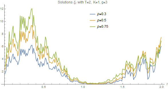
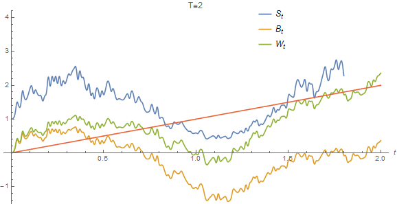
We simulate the trajectories of the Wiener process W~t\widetilde{W}_{t} on time interval [0,2],[0,2], and so we obtain the trajectories of B~t=W~t+(a+1/2)​t\widetilde{B}_{t}=\widetilde{W}_{t}+(a+1/2)t and S~t=exp⁡(B~t−t/2).\widetilde{S}_{t}=\exp(\widetilde{B}_{t}-t/2). We take one of the obtained sample paths of S~t\widetilde{S}_{t} and presented it on Figure 2. By formula (4.14), for this trajectory we construct the sample paths of ξ~t,\widetilde{\xi}_{t}, with g=3g=3 and ρ=0.3,0.5,0.75.\rho=0.3,0.5,0.75. On Figure 1, we present these sample paths, grouped by ρ.\rho.

Values of solutions of equation (3.4), values of 𝔼​(G−G~)2\mathbb{E}(G-\widetilde{G})^{2} and 𝔼P~​G~\mathbb{E}_{\widetilde{P}}\widetilde{G} are presented on Table 1. We see that P~\widetilde{P}-average of GG decreases when ρ\rho increases.

The values of (4.9) are presented on Table 2 and they are naturally decreasing to 0 as g↑𝔼P~​G~.g\uparrow\mathbb{E}_{\widetilde{P}}\widetilde{G}. However, the total risk is always greater the than 𝔼​(G−G~)2\mathbb{E}(G-\widetilde{G})^{2}. On the second part of Table 2 we present sensitivity of (4.9) with respect to gg by computing the following values 1m​i​ni​m​i​ni+1−m​i​nigi+1−gi,\frac{1}{min_{i}}\frac{min_{i+1}-min_{i}}{g_{i+1}-g_{i}}, where m​i​ni=𝔼​(G~−(G~+v⁡(gi)​DT)+)2,min_{i}=\mathbb{E}(\widetilde{G}-(\widetilde{G}+v(g_{i})D_{T})^{+})^{2}, i=1,2,3.i=1,2,3.

Table 1.
Solutions of equation (3.4)
g=0.5 g=1 g=2 g=3
ρ\rho=0.3 83.7419 41.1694 17.2824 9.18066
ρ\rho=0.5 99.4493 40.1427 12.4501 4.90082
ρ\rho=0.75 110.058 31.6334 5.00461 0.60940
Values of problem [S⁡(g,0,G)S({g,0;{G}})]
𝔼​(G−G~)2\mathbb{E}(G-\widetilde{G})^{2} 𝔼P~​G~\mathbb{E}_{\widetilde{P}}\widetilde{G}
ρ\rho=0.3 2497.04 10.0949
ρ\rho=0.5 2315.28 6.50358
ρ\rho=0.75 1738.17 3.67076
Table 2. Minimum values of problem [S⁡(g,0;GCLOSES({g,0;{G}}]
Values of (4.9)
g=0.5 g=1 g=2 g=3
ρ\rho=0.3 361.328 306.613 225.509 165.277
ρ\rho=0.5 412.641 308.070 177.939 98.553
ρ\rho=0.75 506.590 291.153 92.440 15.821
Changes of (4.9)
g=0.5 g=1 g=2
ρ\rho=0.3 -30.3% -26.5% -26,7%
ρ\rho=0.5 -50.7% -42.2% -44.6%
ρ\rho=0.75 -85.1% -68.3% -82.9%
Refer to caption
Figure 1. Sample paths of solutions of minimization problem [S⁡(g,0,G)S({g,0;{G}})] with g=4g=4
Refer to caption
Figure 2. Sample paths of S~,B~,W~\widetilde{S},\widetilde{B},\widetilde{W}

References

  • [Bielecki et al. (2005)] T. R. Bielecki, H. Jin, S. R. Pliska, & X. Y. Zhou (2005) Continuous–time mean‐-variance portfolio selection with bankruptcy prohibition, Mathematical Finance 15(2), 213–244.
  • [Ceci et al. (2014)] C. Ceci, A. Cretarola, & F. Russo (2014) GKW representation theorem under restricted information: An application to risk-minimization, Stochastics and Dynamics 14(02), 1350019 [23 pages].
  • [Černỳ (2004)] A. Černỳ (2004) Dynamic programming and mean-variance hedging in discrete time, Applied Mathematical Finance 11(1), 1–25.
  • [Di Nunno, Øksendal & Proske (2009)] G. Di Nunno, B. K. Øksendal & F. Proske (2009) Malliavin calculus for Lévy processes with applications to finance. Berlin: Springer.
  • [Fischer et al. (1999)] P. Fischer, E. Platen & W. J. Runggaldier (1999) Risk minimizing hedging strategies under partial observation. In Seminar on Stochastic Analysis, Random Fields and Applications, 175–188. Basel:Birkhäuser.
  • [Föllmer & Leukert (2000)] H. Föllmer & P. Leukert (2000) Efficient hedging: cost versus shortfall risk, Finance and Stochastics 4(2), 117–146.
  • [Föllmer & Sondermann (1986)] H. Föllmer & D. Sondermann (1986) Hedging of non-redundant contingent claims. In Contributions to Mathematical Economics (W. Hildenbrand & A. Mas-Colell, eds.), 205–223. North Holland.
  • [Fujii & Takahashi (2014)] M. Fujii & A. Takahashi (2014) Making mean-variance hedging implementable in a partially observable market, Quantitative Finance 14(10), 1709–1724.
  • [Hubalek et al. (2006)] F. Hubalek, J. Kallsen & L. Krawczyk (2006) Variance-optimal hedging for processes with stationary independent increments, The Annals of Applied Probability 16(2), 853–885.
  • [Jeanblanc et al. (2012)] M. Jeanblanc, M. Mania, M. Santacroce & M. Schweizer (2012) Mean-variance hedging via stochastic control and BSDEs for general semimartingales, The Annals of Applied Probability 22(6), 2388–2428.
  • [Korn & Trautmann (1995)] R. Korn & S. Trautmann (1995) Continuous-time portfolio optimization under terminal wealth constraints, Mathematical Methods of Operations Research 42(1), 69–92.
  • [Korn (1997)] R. Korn (1997) Some applications of l2-hedging with a non-negative wealth process, Applied Mathematical Finance 4(1), 65–79.
  • [Lefèvre et al. (2001)] D. Lefèvre, B. Øksendal & A. Sulem (2001) An introduction to optimal consumption with partial observation. In Mathematical Finance, Trends Math. 239–249. Basel:Birkhäuser.
  • [Øksendal (1996)] B. K. Øksendal (1996) An introduction to Malliavin calculus with applications to economics, Norwegian School of Economics and Business Administration, Working Paper.
  • [Schäl (1994)] M. Schäl (1994) On quadratic cost criteria for option hedging, Mathematics of Operations Research 19(1), 121–131.
  • [Schweizer (1992)] M. Schweizer (1992) Mean-variance hedging for general claims, The Annals of Applied probability 2(1), 171–179.
  • [Schweizer (1994)] M. Schweizer (1994) Risk-minimizing hedging strategies under restricted information, Mathematical Finance 4(4),  327–342.
  • [Schweizer (1995)] M. Schweizer (1995) Variance-optimal hedging in discrete time, Mathematics of Operations Research 20(1),  1–32.
  • [Weisshaupt (2003)] H. Weisshaupt (2003) Insuring against the shortfall risk associated with real options. Decisions in Economics and Finance 26(2),  81–96.